Spatial and Temporal Variability of Iodine in AerosolJuan Carlos Gómez Martín

(1)

1. Introduction

Iodine is a key element in mammalian metabolism whose major global source is oceanic surface gas emissions of iodine-bearing molecules to the atmosphere (Whitehead, 1984). The photooxidation of these compounds leads to chemical cycles that impact the oxidative capacity of the atmosphere and to the partitioning of the iodine load to aerosol (Saiz-Lopez, Lamarque, et al., 2012; Saiz-Lopez, Plane, et al., 2012), which is the main carrier of this element toward continental food chains (Whitehead, 1984). Even though the enrichment of marine aerosol in iodine is well established (I/Na ratio several hundred times that of bulk

Abstract

In this work, we describe the compilation and homogenization of an extensive data set of aerosol iodine field observations in the period between 1963 and 2018 and we discuss its spatial and temporal dependences by comparison with CAM-Chem model simulations. A close to linear relationship between soluble and total iodine in aerosol is found (∼80% aerosol iodine is soluble), which enables converting a large subset of measurements of soluble iodine into total iodine. The resulting data set shows a distinct latitudinal dependence, with an enhancement toward the Northern Hemisphere (NH) tropics and lower values toward the poles. This behavior, which has been predicted by atmospheric models to depend on the global distribution of the main oceanic iodine source (which in turn depends on the reaction of ozone with aqueous iodide on the sea water-air interface, generating gas-phase I2 and HOI), is confirmed here by field observations for the first time. Longitudinally, there is some indication of a wave- one profile in the tropics, which peaks in the Atlantic and shows a minimum in the Pacific. New data from Antarctica show that the south polar seasonal variation of iodine in aerosol mirrors that observed previously in the Arctic, with two equinoctial maxima and the dominant maximum occurring in spring.

While no clear seasonal variability is observed in NH middle latitudes, there is an indication of different seasonal cycles in the NH tropical Atlantic and Pacific. Long-term trends cannot be unambiguously established as a result of inhomogeneous time and spatial coverage and analytical methods.

Plain Language Summary

Iodine is a key trace element in continental food chains whose major global source is oceanic surface gas emissions of iodine-bearing molecules to the atmosphere.

Atmospheric chemical processing of these substances is followed by incorporation of the iodine-bearing products into airborne marine aerosol particles, which are the carriers of iodine to the continents. In this work, we compile a data set of aerosol composition measurements reporting iodine concentrations at many different locations, seasons, and years. Analysis of the variation of the concentration iodine in aerosol with latitude and longitude enables us to confirm the main mechanism emitting iodine from the oceans, which is triggered by deposition of ozone on the water-air interface. In addition, we analyze the seasonal variation of the iodine concentration in aerosol in different locations, which also sheds light onto additional iodine sources to the atmosphere. Finally, long-term trends cannot be unambiguously established, but the observations are compatible with the model-predicted enhancement of aerosol iodine as a result of increased oceanic iodine emissions over the last 50 years related to ozone pollution.

This is an open access article under the terms of the Creative Commons Attribution-NonCommercial License, which permits use, distribution and reproduction in any medium, provided the original work is properly cited and is not used for commercial purposes.

Rafael P. Fernandez³ , Benjamin Gilfedder⁴ , Rolf Weller⁵, Alex R. Baker⁶ , Elise Droste^6,7 , and Senchao Lai⁸

1Instituto de Astrofísica de Andalucía, CSIC, Granada, Spain, ²Department of Atmospheric Chemistry and Climate, Institute of Physical Chemistry Rocasolano, CSIC, Madrid, Spain, ³Institute for Interdisciplinary Science, National Research Council (ICB-CONICET), FCEN-UNCuyo, Mendoza, Argentina, ⁴Limnological Research Station, University of Bayreuth, Bayreuth, Bayern, Germany, ⁵Department of Glaciology, Alfred-Wegener-Institut Helmholtz Zentrum für Polar- und Meeresforschung, Bremerhaven, Germany, ⁶Centre for Ocean and Atmospheric Science, School of Environmental Sciences, University of East Anglia, Norwich, UK, ⁷Department of Environmental Sciences, Wageningen University and Research Centre, Wageningen, The Netherlands, ⁸South China University of Technology, School of Environment and Energy, Higher Education Mega Center, Guangzhou, China

Key Points:

• Soluble aerosol iodine field observations can be combined with total aerosol iodine data to build a longer term global homogenized data set

• Soluble iodine represents approximately 80% of total aerosol iodine, while aerosol iodine amounts to about 30% of total atmospheric iodine

• The spatial distribution of aerosol iodine provides the first global-scale observational evidence of the major source of atmospheric iodine

Supporting Information:

Supporting Information may be found in the online version of this article.

Correspondence to:

J. C. Gómez Martín and A. Saiz-Lopez, jcgomez@iaa.es;

a.saiz@csic.es

Citation:

Gómez Martín, J. C., Saiz-Lopez, A., Cuevas, C. A., Fernandez, R. P., Gilfedder, B., Weller, R., et al. (2021).

Spatial and temporal variability of iodine in aerosol. Journal of Geophysical Research: Atmospheres, 126, e2020JD034410. https://doi.

org/10.1029/2020JD034410 Received 12 DEC 2020 Accepted 5 APR 2021

Author Contributions:

Conceptualization: Juan Carlos Gómez Martín, Alfonso Saiz-Lopez Data curation: Juan Carlos Gómez Martín, Benjamin Gilfedder, Alex R.

Baker, Elise Droste, Senchao Lai Formal analysis: Juan Carlos Gómez Martín, Benjamin Gilfedder, Alex R.

Baker

(2)

seawater) and has been documented in early works on atmospheric iodine chemistry (see Duce et al., 1965, and references therein), the specific processes controlling the phase-partitioning remain unknown. Uptake of gas-phase iodine compounds on sea-salt aerosol is believed to be responsible for this large enrichment (Duce et al., 1983). This, however, is not an irreversible sink for iodine, since chemical processes analogous to those leading to the release of iodine-bearing gases from the sea surface (Carpenter et al., 2013; Garland

& Curtis, 1981; MacDonald et al., 2014; Miyake & Tsunogai, 1963) occur as well on air–aqueous aerosol interfaces (Magi et al., 1997).

Iodine in aerosol has received less attention than gas-phase iodine and its chemistry remains poorly un- derstood (Saiz-Lopez, Plane, et al., 2012). Uptake of iodine oxides (IxOy) and oxyacids (HOIx), as well as of iodine nitrate (IONO2) and nitrite (IONO) on aerosol surfaces remains to be studied more thoroughly both experimentally and theoretically. The processing and partitioning between water insoluble and soluble iodine species, between soluble organic and inorganic iodine, and in the latter group between aqueous iodide (I⁻) and iodate (IO3−) are essentially unknown. This includes the formation of volatile species that can go back to the gas phase (recycling), which is thought to occur via I⁻, and the formation of species assumed to be stable and unreactive, that is, iodate IO3− (Vogt et al., 1999). The existing aerosol chemical schemes cannot explain the speciation variability and the relative concentrations of iodide and iodate observed in the field. The aerosol I⁻ concentration is predicted to be negligible as a result of recycling to the gas phase, while IO3− is predicted to accumulate in particles (Pechtl et al., 2007; Vogt et al., 1999). However, many field observations show a significant I⁻ concentration in aerosol samples (Baker, 2004, 2005; Gäbler & Heu- mann, 1993; Lai et al., 2008; Wimschneider & Heumann, 1995; Yu et al., 2019).

Despite the many existing unknowns about aerosol iodine chemistry and speciation, the total iodine (TI) content of aerosol can be expected to gauge the strength of the iodine oceanic emissions and thus provide a sense of how these vary with location and time. Currently, the major source of iodinated gases to the troposphere is believed to be the reaction of gas-phase O3 with I⁻ on the seawater-air interface. This assessment is mainly based on laboratory work (Carpenter et al., 2013; Garland & Curtis, 1981; MacDonald et al., 2014) and the ability of global models to reproduce the observations of gas-phase iodine monoxide (IO) at a few locations (Saiz-Lopez et al., 2014; Sherwen, Evans, Carpenter, et al., 2016). In addition, Sherwen, Evans, Spracklen, et al. (2016) used a set of TI and total water-soluble iodine (TSI) open ocean observations to test the performance of global simulations of tropospheric iodine aerosol with GEOS-Chem, obtaining broad agreement with the relatively sparse cruise data considered. These simulations predict the highest TI to occur in the tropical marine boundary layer (MBL), as a result of the latitudinal dependence of iodine gas source emissions (Prados-Roman et al., 2015) that results from the superposition of the seawater I⁻ and gas-phase O3 distributions.

A wealth of field observations of TI in bulk aerosol and fine and coarse aerosol, as well as of iodine speciation exist (Figure 1). These results, however, are scattered in the literature and no attempt of putting togeth- er a comprehensive database and investigating its spatial and temporal variability has been carried out to the best of our knowledge. A list of TI and soluble iodine speciation observations was compiled for a previous review of atmospheric iodine chemistry (Saiz-Lopez, Plane, et al., 2012), but some important historic data sets were missed (e.g., all the PEM WEST A results), and new cruise and ground-based observations are currently available. There are reasons to exclude TI observations at coastal and island stations from a comparison with global simulations, for example, observations may be biased by locally intensive biogenic emissions with respect to oceanic observations, which are sensitive to less intensive but more widespread sources of iodine. However, the sparsity of the cruise data and its concentration mostly in the Atlantic sug- gests resorting to the abundant data obtained from ground-based stations.

The present paper deals with the compilation of a global aerosol TI data set including both cruise and ground-based (coastal and insular) observations and the analysis of its spatial and temporal trends. The data set includes unpublished aerosol iodine data obtained from the analysis of samples collected at Neumayer II Station (Antarctica) (Weller et al., 2008) and during a short cruise around the island of Monserrat in the tropical Atlantic (Lin et al., 2016), as well as data obtained in three cruises that have only been fully reported in two PhD theses and a MSc thesis (Droste, 2017; Lai, 2008; Yodle, 2015), and an improved analysis and extended version of the TI data of the 23rd Chinese Antarctic Campaign cruise (Gilfedder et al., 2010; Lai et al., 2008). Community Atmospheric Model with chemistry (CAM-Chem) global simulations are then

Investigation: Juan Carlos Gómez Martín, Rolf Weller, Alex R. Baker, Elise Droste, Senchao Lai

Methodology: Juan Carlos Gómez Martín, Carlos A. Cuevas, Rafael P.

Fernandez, Benjamin Gilfedder, Rolf Weller, Alex R. Baker, Elise Droste, Senchao Lai

Resources: Juan Carlos Gómez Martín, Carlos A. Cuevas, Alex R. Baker Software: Carlos A. Cuevas, Rafael P.

Fernandez

Supervision: Juan Carlos Gómez Martín

Visualization: Juan Carlos Gómez Martín, Carlos A. Cuevas

Writing – original draft: Juan Carlos Gómez Martín

Writing – review & editing: Juan Carlos Gómez Martín, Alfonso Saiz- Lopez, Carlos A. Cuevas, Rafael P.

Fernandez, Benjamin Gilfedder, Rolf Weller, Alex R. Baker, Senchao Lai

(3)

employed to test the performance of the model in reproducing these trends and distributions, with the purpose of highlighting the existing uncertainties and/or the importance of including missing processes in global simulations. Iodine partitioning between coarse and fine aerosol and speciation will be discussed in a follow-up publication. A spreadsheet containing the compiled data can be found in the supplementary information.

2. Methods

2.1. Definitions

The TI concentration (in pmol m⁻³) is defined as the amount of particulate iodine collected by a filter or collection surface per volume unit of sampled air. Extraction methods may use a solvent (usually water) to facilitate the analysis. Thus, TI is the sum of TSI plus nonsoluble iodine (NSI), that is, TI = TSI + NSI. TSI comprises total inorganic iodine (TII = I⁻ + IO3−) and soluble organic iodine (SOI), that is, TSI = TII + SOI.

Total gas-phase iodine (TIy) consist of the sum of organic iodine (GOI) and inorganic iodine (Iy) in the gas phase, that is, TIy = GOI + Iy. Table 1 lists the acronyms used throughout this work and the corresponding definitions.

Aerosol size-segregated observations of TI and/or TSI have been reported by means of set of stacked filters or by using cascade impactors (CIs) (Duce et al, 1965, 1967; Gilfedder et al., 2008). The bulk TI concentration is the sum of the TI within each size range. Usually, aerosol TI is reported for coarse (diameter d > 1 μm) and fine (d < 1 μm) aerosol, and TIbulk = TIfine + TIcoarse. There are, however, other studies where TI in particulate matter with d ≤ 2.5 μm (PM2.5) collected by virtual impactors (VIs) is reported (Gilfedder et al., 2008). When collecting filters are used, typical extraction procedures include thermal extraction, ultrasonication, and mechanical shaking (Yodle & Baker, 2019). In combination with these methods for measuring TI in aerosol, techniques for capturing gas-phase Iy and TIy have also been implemented. For Iy, the air flow may be passed additionally through filters impregnated in alkaline substances (Gäbler & Heu- mann, 1993; Rancher & Kritz, 1980) or bubbled through an alkaline solution (Duce et al., 1965). For TIy, a combination of an electrostatic precipitator and a charcoal trap has been used (Moyers & Duce, 1972, 1974).

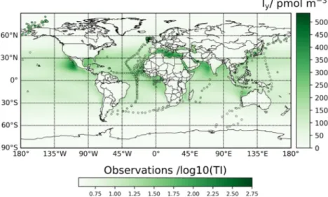
A more modern method for determining the concentration of iodocarbons is gas chromatography–mass Figure 1. Geographical distribution of total iodine (TI) and total soluble iodine (TSI) observations. Stations: yellow triangles; cruises: color-coded dots (see legend). The SEAREX cruise region is shown in shaded, because the aerosol sampling points are not available (only the average TI for the second leg of the cruise was reported).

(4)

spectrometry analysis of air samples stored in canisters, but it does not appear to have been applied to measure the overall airborne iodine budget.

The analytical method most widely used to quantify TI in older observations is instrumental neutron activation analysis (INAA) (Arimoto et al., 1989, 1996; Duce et al., 1965, 1973). Isotope dilution mass spectrometry (IDMS) has also been used to determine TI (Gäbler & Heumann, 1993). Contemporary observations employ more accessible techniques such as thermal extraction with spectrometric detection (TESI) of iodine (Gilfedder et al., 2010) for TI and inductively coupled plasma-mass spectrometry (ICP-MS) for TSI (Baker, 2005; Lai et al., 2008).

2.2. Description of Data Sets 2.2.1. Geographical Distribution

We have compiled iodine aerosol data from 55 field campaigns across the globe spanning 55 years (1963–

2018), consisting of 7,794 datapoints (Supplementary Information). Of these, 7,772 are measurements of individual samples and the remaining 22 points are the reported averages of a total of 510 samples which we have not been able to retrieve. Since the source of iodine is mainly marine, only ship-borne, coastal, or insular campaigns have been considered. Tables 2 and 3 list the 19 cruises (C#) and 36 coastal ground-based (S#) campaigns where aerosol iodine measurements have been carried out. Totally or partially unpublished aerosol TI and TSI data included in our compilation (C7, C8, C12, C14, C17, C18, and S33) are described in the supporting information S1.

Figure 1 shows the geographical distribution of these observations. The data set samples well the latitudinal coordinate. Longitudinally, most observations are concentrated in the Atlantic, while there is a complete lack of data in the eastern Pacific. Some locations need to be considered carefully, since they may be affected by locally enhanced sources of iodine. For example, there is evidence that the MAP 2006 (Gilfedder et al., 2008; Lai, 2008) data (S32) is affected by intense particle formation following biogenic emissions.

Similarly, the decline of Arctic sea ice may have enhanced airborne iodine in C13 with respect to C7 (Kang et al., 2015). Also, aerosol sampled in the free troposphere (S1c, S1d, S7, and S17) is likely to show different iodine content than at sea level.

2.2.2. Types of Data

Most of the samples were analyzed for TI, but in some of the recent works TSI analysis was reported (C4, C6, C8–C10, C14, C17–C19, S32, and S36). Fortunately, the samples of some cruises (C5, C7, and C11–C13) and ground-based campaigns (S14, S34, and S35) were analyzed for both TI and TSI, which allows obtaining a relationship between both quantities to convert TSI into TI (see Section 3.1). Similarly, most works report bulk aerosol measurements. Only two cruises (C8 and C9) reported exclusively PM2.5 measurements. Again, CI size-segregated data are available for several campaigns (S1, S2, S4, S9, S20, and S32), which enables to

Acronym/symbol Definition

TI Total iodine (in aerosol)

NSI Nonsoluble iodine (in aerosol)

TSI Total soluble iodine (in aerosol)

TII Total inorganic iodine (in aerosol)

SOI Soluble organic iodine (in aerosol)

Xbulk, Xfine, Xcoarse (X = TI, TSI) Iodine in bulk aerosol and in the fine and coarse aerosol fractions

TIx, TSIx TI and TSI for d < x μm

TIy Total iodine (gas phase)

Iy Inorganic iodine (gas phase)

GOI Gas-phase organic iodine

Table 1

Definition of Iodine Variables

(5)

# Program/

campaign Cruise Location Min

lon Max lon Min

lat Max lat Date

start Date end N Type of data Methods Reference

C1 R/V Capricorne Equatorial

Atlantic −2.7 9.2 −5.2 2.7 30-05-77 12-06-77 24 TI (bulk), Iy INAA Rancher and Kritz (1980) C2 SEAREX Westerlies, R/V

Moana Wave North

Pacific −170 −149 22 40 10-06-86 11-07-86 17 TI (bulk) INAA Arimoto et al. (1989) C3 Polarstern

CampaignsANT-VII/5 (PS14),

R/V Polarstern Tropical

Atlantic −1 2 −11 −6 18-03-89 18-03-89 1 I⁻, IO3− (bulk) IDMS Wimschneider and Heumann (1995) C4 German

SOLAS M55, R/V Meteor Tropical

Atlantic −56.2 −3.5 0.1 11.3 15-10-02 13-11-02 28 TSI

(fine + coarse) CI^b; ICP-

MS Baker (2005) C5 CHINARE 2nd CHINARE,

R/V Xue-long Western Pacific–

Arctic Ocean

121 −150 35.0 80.0 15-07-03 26-09-03 44 TI, TSI (bulk) ICP-MS Kang et al. (2015)

C6 AMT AMT13 RRS

James Clark Ross

Atlantic

Transect −40.2 −14.3 −41.1 47.3 14-09-03 08-10-03 22 TSI

(fine + coarse) CI^b; ICP-MS

Baker (2005)

C7 CAC 23rd CAC R/V

Xue-Long Western Pacific–

Indian–

Southern Ocean

70.8 122.0 −69.3 26.2 20-11-05 22-03-06 57 TI, TSI (bulk) TESI, ICP-MS

Gilfedder

et al. (2010), Lai et al. (2008), this work C8 MAP CEC, R/V Celtic

Explorer North

Atlantic −12.3 −7.5 50.7 57.4 12-06-06 05-07-06 33 TSI (PM2.5) VI; IC- ICP-MS

Gilfedder et al. (2008), Lai (2008) C9 OOMPH VT 88 R/V Marion

Dufresne Southern

Atlantic −59.2 15.8 −44.9 −33.7 20-01-07 02-02-07 14 TSI (PM2.5) ICP-MS Lai et al. (2011) C10 RHaMBLe RRS Discovery

D319 East

Tropical Atlantic

−23.1 −14.1 16.6 33.3 22-05-07 05-06-07 14 TSI

Allan et al. (2009)

C11 UK-SOLAS INSPIRE RRS Discovery D325

Eastern Tropical North Atlantic

−25.0 −22.8 16.0 26.0 17-11-07 16-12-07 17 TI, TSI (bulk) TESI Gilfedder et al. (2010), Sherwen, Evans, Spracklen, et al. (2016)

C12 RRS James Cook

Cruise 18 (JC18)

Tropical

Atlantic −63 −62.5 16.2 16,7 04-12-07 14-12-07 8 TI, TSI

This work

C13 CHINARE 3rd CHINARE,

R/V Xue-long Western Pacific–

Arctic Ocean

122 −146 31.2 85.1 13-07-08 21-09-08 28 TI, TSI (bulk) ICP-MS Xu et al. (2010)

C14 TransBrom R/V Sonne

SO202-2 Tropical Western Pacific

143.7 154.5 −14.6 36.0 10-10-09 22-10-09 13 TSI

Yodle (2015)

C15 UK-

GEOTRACESRRS Discovery

D357 Southern

Atlantic −3.6 17.3 −40.0 −34.5 18-10-10 19-11-10 11 TI (bulk) INAA Sherwen, Evans, Spracklen, et al. (2016) C16 UK-

GEOTRACES RRS Discovery

D361 Atlantic

transect −28.8 −17.8 −6.6 22.3 21-02-11 16-03-11 24 TI (bulk) INAA Sherwen, Evans, Spracklen, et al. (2016)

C17 AMT AMT21 RRS

Discovery D371

Atlantic

Transect −51.0 −16.4 −45.1 48.2 01-10-

11 07-11-11 33 TSI

Yodle (2015) Table 2

List of Cruises Reporting Aerosol Iodine^a

(6)

deduce a relationship between TI2–3 and TIbulk. Regarding gas-phase measurements, campaigns C1, S1, S5, S6, and S29 report measurements of Iy or TIy.

2.2.3. Quality of Data

Sample data availability: In some cases, the individual sample data (C3, S8, S10, S28, and S29) are plotted in the original publication, but no longer available or not accessible in digital form. In these cases, the data have been digitized from the plots in the original papers. In newer publications, digitization of plots with many datapoints can be done with good accuracy (e.g., S28), but in older papers this is not always the case.

For Mould Bay (S8) and Igloolik (S10), the data are affected by the clustering of the symbols in the plot and some points may be missing because of fading symbols in the hard copy from which the papers were scanned. Thus, the number of samples and the actual values may differ from the original data, although the overall campaign statistics are close to those of the original data.

Only campaign statistics reported: Comparing cruise and ground-based measurements is often difficult, since cruise observations are snapshots of the state of the atmosphere, while ground-based observations enable much longer integration times. Some papers report only statistics of long-term sampling and do not provide the individual measurements (C2, S7, S12, S13, S20, S30, and S36). Moreover, the statistics provided in different works may differ (e.g., for S12 the geometric mean is reported instead of the arithmetic mean).

This may cause a problem of consistency in the treatment of the full data set. In the present paper, we use the arithmetic mean and we have estimated it if not available.

Data below detection limit. We are aware of a campaign in coastal Australia (MUMBA) where TI measure- ments with ion beam analysis–particle induced X-ray emission (IBA-PIXE) were carried out (Paton-Walsh et al., 2017). The concentrations determined were below a detection limit of ∼1.2 nmol m⁻³ (P. Davy, per- sonal communication), which is 2 orders of magnitude higher than typical TI concentrations measured in the same region (∼10 pmol m⁻³, campaigns S12 and S13). Thus, we are unable to use this data set.

2.3. Model Description

The halogen version of the global 3-D chemistry-climate model CAM-Chem (version 4) (Fernandez et al., 2014; Saiz-Lopez et al., 2014) has been used to calculate the reactive and total gas-phase iodine budget.

The model setup includes a state-of-the-art emissions inventory and chemistry scheme for halogens (cho- rine, bromine, and iodine) (Fernandez et al., 2014; Saiz-Lopez et al., 2014). Briefly, the iodine chemical scheme includes an independent representation of dry and wet deposition for each inorganic gas-phase iodine species (I, I2, IO, OIO, INO, INO2, IONO2, HI, HOI, I2O2, I2O3, I2O4, IBr, and ICl), which are termed collectively as Iy. The organic iodine sources from a top-down emission inventory (Ordóñez et al., 2012) represent the oceanic emissions and photochemical breakdown of four iodocarbons (CH3I, CH2ICl, CH2IBr,

# Program/

campaign Cruise Location Min

lon Max lon Min

lat Max lat Date

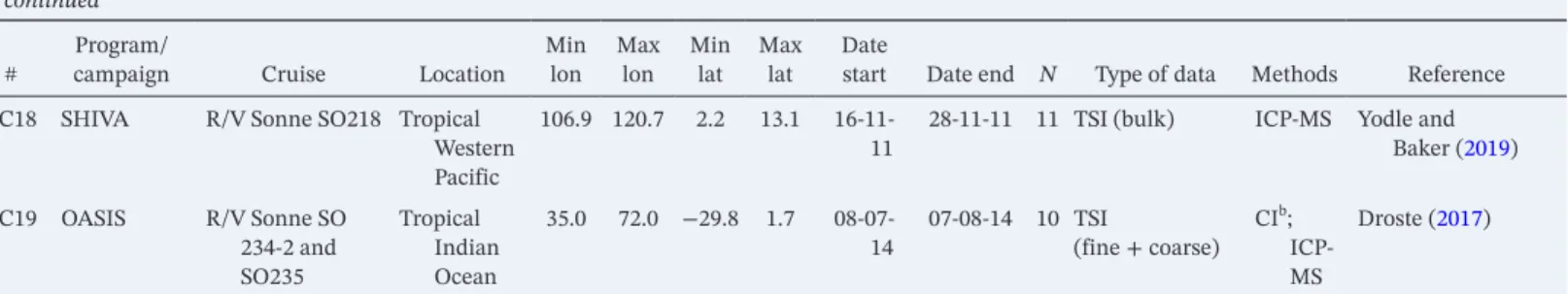
start Date end N Type of data Methods Reference C18 SHIVA R/V Sonne SO218 Tropical

Western Pacific

106.9 120.7 2.2 13.1 16-11-

11 28-11-11 11 TSI (bulk) ICP-MS Yodle and Baker (2019) C19 OASIS R/V Sonne SO

234-2 and SO235

Tropical Indian Ocean

35.0 72.0 −29.8 1.7 08-07-

14 07-08-14 10 TSI

Droste (2017)

aAbbreviations: SOLAS, Surface-Ocean/Lower Atmosphere Study; AMT, Atlantic Meridional Transect; CHINARE, China National Arctic Research Expedition;

CAC, China Antarctic Campaign; MAP, Marine Aerosol Production from Natural Sources; OOMPH, Organics over the Ocean Modifying Particles in both Hemispheres; RHaMBLe, Reactive Halogens in the Marine Boundary Layer; SHIVA, Stratospheric Ozone: Halogen Impacts in a Varying Atmosphere; OASIS, Organic very short lived substances and their Air Sea Exchange from the Indian Ocean to the Stratosphere; CI, cascade impactor; VI, virtual impactor; INAA, instrumental neutron activation analysis; ICP-MS, inductively coupled plasma-mass spectrometry; IDMS, isotope dilution mass spectrometry; TESI, thermal extraction with spectrometric detection.

bCascade impactors were also used to achieve the coarse/fine separation, but they were not used to achieve detailed size segregation.

Table 2 continued

(7)

# Program/

campaign Location Lon Lat Date

start Date

end N Type of data Methods Reference

S1a Hilo, HI, USA −155.1 19.9 27-05-63 18-06-63 5 TI (size

segregated), Iy

CI; INAA Duce et al. (1965)

S1b Mauna Loa, HI,

USA (600 m) −155.6 19.9 05-06-63 25-06-63 2

S1c Mauna Loa, HI,

USA (2,000 m) −155.6 19.9 05-06-63 25-06-63 1

S1d Mauna Loa, HI,

USA (3,300 m) −155.6 19.9 05-06-63 25-06-63 1

S2 Cambridge, MA,

USA −71.1 42.4 31-10-64 14-11-64 10 TI (size

segregated) CI; INAA Lininger et al. (1966)

S3 Barrow, AK, USA −156.8 71.3 20-01-65 28-01-65 23 TI (bulk) INAA Duce et al. (1966)

S4 Hilo, HI, USA −155.1 19.9 01-08-66 31-08-66 8 TI (size

segregated) CI; INAA Duce et al. (1967)

S5 Oahu, HI, USA −157.7 21.3 01-08-69 10-08-69 11 TI (bulk), TIy INAA Moyers and

Duce (1972)

S6 McMurdo,

Antarctica 166.7 −77.8 08-11-70 12-12-70 19 TI (bulk), TIy INAA Duce et al. (1973)

S7 Mauna Loa, HI,

USA (3,300 m) −155.6 19.9 01-02-79 31-05-85 287 TI (bulk) INAA Zieman et al. (1995)

S8 CAASN Mould Bay,

Canada −119.3 76.2 11-04-79 20-05-82 135 TI (bulk) INAA Sturges and

Barrie (1988)

S9 SEAREX Enewetak,

Marshall Islands

162.0 11.5 18-04-79 04-08-79 27 TI (size

segregated) CI; INAA Duce et al. (1983)

S10 CAASN Igloolik, Canada −81.7 69.4 29-10-79 16-05-82 110 TI (bulk) INAA Sturges and

Barrie (1988)

S11 CAASN Alert, Canada −62.3 82.5 13-07-80 18-12-06 1,234 TI (bulk) INAA Sharma et al. (2019)

S12a SEAREX American Samoa

ISS −170.6 −14.3 01-01-81 31-08-81 7 TI (bulk) INAA Arimoto et al. (1987)

S12b SEAREX American Samoa

OSS −170.6 −14.3 01-01-81 31-08-81 4 TI (bulk) INAA Arimoto et al. (1987)

S13 SEAREX New Zealand 172.7 −34.4 01-05-83 31-08-83 11 TI (bulk) INAA Arimoto et al. (1990)

S14 Tokyo, Japan 139.8 35.7 14-07-83 23-03-84 9 TI, TSI (bulk) INAA Hirofumi et al. (1987)

S15 AEROCE Tudor Hill,

Bermuda, UK −64.87 32.24 29-07-88 26-12-97 1,308 TI (bulk) INAA Arimoto et al. (1995) S16 AEROCE Ragged Point,

Barbados −59.4 13.2 17-08-88 30-12-97 2,750 TI (bulk) INAA Arimoto et al. (1995) S17 AEROCE Izaña, Tenerife,

Spain (2360 m)

−16.5 28.3 17-06-89 28-12-97 905 TI (bulk) INAA Arimoto et al. (1995)

S18 AEROCE Mace Head,

Ireland −9.73 53.3 07-08-89 15-08-94 436 TI (bulk) INAA Huang et al. (2001)

S19 Ibaraki, Japan 140.3 36.3 19-02-90 13-05-91 13 TI (bulk) INAA Yoshida and

Muramatsu (1995) S20a Uto, Finland 21.4 59.8 29-04-91 12-05-91 35 TI (fine + coarse) Two filters, INAA Jalkanen and

Manninen (1996) S20b Virolahti, Finland 27.7 60.6 10-06-91 30-06-91 35 TI (fine + coarse)

S21 PEM West

A Midway Island −177.4 28.2 27-05-91 02-12-91 12 TI (bulk) INAA Arimoto et al. (1996)

Table 3

Campaigns in Coastal and Island Stations Reporting Aerosol Iodine Measurements

(8)

and CH2I2), including a cyclic seasonal variation. Inorganic sources of iodine (HOI and I2 emitted from the ocean surface) are based on laboratory studies of the oxidation of aqueous iodide by surface ozone reacting on the ocean’s surface (Carpenter et al., 2013; MacDonald et al., 2014) and are computed online using sea surface temperature (SST) as a proxy (Prados-Roman et al., 2015). In this work, we use the output from a REF-C1 model run used previously to simulate the evolution of iodine concentration in the RECAP ice core (coastal East Greenland) (Cuevas et al., 2018). CAM-Chem was configured with a horizontal resolution of 1.9° latitude by 2.5° longitude and 26 vertical levels from the surface to the stratosphere (∼40 km). The model was run in free-running mode considering prescribed SST fields and sea ice distributions from 1950 to 2010 (Tilmes et al., 2016), which covers the major part of the time span of observations (1963–2018).

Therefore, the model dynamics and transport represent the daily synoptic conditions of the observations and allow the direct online coupling between the ocean, ice, and atmospheric modules during the 60 years of simulation. A land-mask filter (land fraction < 1.0) has been applied to all longitudinal and latitudinal averages from the model output, in order to account only for coastal and open ocean regions.

Table 3 Continued

# Program/

campaign Location Lon Lat Date

start Date

end N Type of data Methods Reference

S22 PEM West

A Hong Kong,

China 114.3 22.6 06-09-91 25-11-91 50 TI (bulk) INAA Arimoto et al. (1996)

S23 PEM West

A Ken-Ting; Taiwan 120.9 21.9 08-09-91 23-10-91 29 TI (bulk) INAA Arimoto et al. (1996)

S24 PEM West

A Okinawa, Japan 128.3 26.9 09-09-91 09-12-91 8 TI (bulk) INAA Arimoto et al. (1996)

S25 PEM West

A Cheju Island;

Korea 126.48 33.52 10-09-91 02-10-91 6 TI (bulk) INAA Arimoto et al. (1996)

S26 PEM West

A Oahu, HI, USA −157.7 21.3 18-09-91 31-10-91 37 TI (bulk) INAA Arimoto et al. (1996)

S27 PEM West

A Shemya, AK, USA 174.1 52.9 19-09-91 31-10-91 15 TI (bulk) INAA Arimoto et al. (1996)

S28 PSE Alert, Canada −62.3 82.5 22-01-92 15-04-92 85 TI (fine + coarse) VI; INAA Barrie et al. (1994)

S29 Weddell Sea

(Filchner Station)

−50.2 −77.1 30-01-92 10-02-92 2 TI (coarse), Iy,

GOI IDMS Gäbler and

Heumann (1993)

S30 Hong Kong,

China 114.2 22.3 01-04-95 30-04-96 114 TI (bulk) INAA Cheng et al. (2000)

S31 Weybourne, UK 1.1 52.9 08-08-96 21-10-97 16 TI (bulk and size

segregated) CI; INAA Baker et al. (2000)

S32 MAP Mace Head,

Ireland −9.7 53.3 13-06-06 06-07-06 75 TSI (fine + coarse,

PM2.5) CI, VI; ICP-MS Gilfedder et al. (2008), Lai (2008)

S33 Neumayer II,

Antarctica −8.3 −70.7 08-01-07 28-01-08 56 TSI (bulk) ICP-MS This work

S34 MAP Mace Head,

Ireland −9.7 53.3 18-06-07 02-07-07 3 TI, TSI (bulk) TESI, INAA Gilfedder et al. (2010)

S35 Riso, Denmark 12.1 55.693 02-04-11 11-12-14 8 TI, TSI (bulk) ICP-MS Zhang et al. (2016)

S36 Xiangshan Gulf,

Zhejiang, China

121.8 29.5 11-02-18 11-05-18 3 TSI (fine and

bulk) Nano-MOUDI; LC-

MS; ICP-MS Yu et al. (2019) Note. SEAREX, Sea/Air Exchange; CAASN, Canadian Arctic Aerosol Sampling Network; PSE, Polar Sunrise Experiment; AEROCE, Atmospheric/Ocean Chemistry Experiment; PEM West A, Pacific Exploratory Mission – West A; American Samoa data ISS, inside selected sector, OSS, outside selected sector. Dates in italics: the original paper does not report exact dates, only months or season. CI, cascade impactor; VI, virtual impactor; nano-MOUDI, Nano-Microorifice Uniform Deposit Impactor; INAA, instrumental neutron activation analysis; ICP-MS, inductively coupled plasma-mass spectrometry; IDMS, isotope dilution mass spectrometry; LC-MS, liquid chromatography mass spectrometry; TESI, thermal extraction with spectrometric detection.

(9)

The 1950–2010 REF-C1 simulation used for model validation did not include the recent implementation of iodine sources and heterogeneous recycling occurring within the polar regions, which strongly affect the total gas-phase Iy burden within the Arctic and Antarctica. Indeed, the de- velopment of the halogen polar module within CAM-Chem (Fernandez et al., 2019) has only been applied to present time conditions and is based on a seasonal sea ice climatology representative of the 2000th decade. Thus, and for the sake of highlighting the large differences on the surface iodine mixing ratios when additional polar sources and chemistry are considered, the perpetual 2000 CAM-Chem output from Fernandez et al. (2019) has also been used to evaluate the model performance at high latitudes.

Although a detailed treatment of uptake, recycling, and loss of individual Iy gas-phase species on sea-salt aerosol and ice-crystals is included in CAM-Chem (Saiz-Lopez et al., 2014, 2015), the model does not track any aerosol iodine species nor the TI content in other types of aerosol.

Note that the accumulation of iodine in aerosol depends on a number unknown or highly uncertain chemical processes that require further investigation, for example, the redox chemistry that may enable intercon- version between IO3− (currently believed to be a sink) and I⁻ (currently thought to lead to recycling of gas-phase iodine), or the role of organic iodinated compounds as I⁻ reservoirs (Saiz-Lopez, Plane, et al., 2012).

Currently, models are essentially unable to explain the speciation of iodine in aerosol, and in particular iodide concentrations are ∼2 orders of magnitude lower than observations (Pechtl et al., 2007). Since Iy uptake on aerosol determines the partitioning of iodine between Iy and TI, it is expected that both quantities show similar spatial and temporal trends.

Therefore, in this work, we have used the modeled Iy to compare with the aerosol TI observations. In doing so, we have scaled the model Iy abundance by the Iy/TI and TIy/TI ratios computed from all cruises and campaigns where both total gas-phase and aerosol iodine were measured, as described below in Section 3.2. Two caveats to this comparison at high latitudes are that the polar module is not fully tested due to sparse gas- phase iodine measurements (especially in the Arctic region) and that the iodine budget is controlled by heterogeneous recycling on ice and loss to iodine oxide particles (IOPs). The later process is not yet implemented in the polar module, and this may lead to a significant overestimation of gas-phase iodine.

3. Results

3.1. Homogenization of Total Iodine Data

In order to study TI spatial and time dependencies, the data need to be homogenized. We use observed TI data if available and derive TI from TSI when TI measurements are not available but TSI was reported instead. This is especially critical for most of the recent cruise samples, for which only TSI was measured (C4, C6, C8–C10, C14, C17–C19, C32, C36, and S33). Similarly, measurements of fine particulate matter or PM2.5

(C8 and C9) need to be scaled to make them directly comparable to bulk aerosol measurements.

Figure 2a displays TI/TSI ratios in bulk aerosol for seven campaigns where both TI and TSI were measured (C5, C7, C11–C13, S14, S34, and S35). Figure 2b demonstrates that a strong linear correlation exists between bulk TI and TSI (Figure S1a shows the same plot in a liner scale). We exclude from this analysis seven (TI, TSI) pairs (four of C7 and three of C12) for which TI/TSI < 1 beyond 2σ analytical uncertainty (i.e., overes- timated TSI). The regression line (considering error in both coordinates) is given by

   

³  ³   ³

TI / pmol m 2.1 0.4 / pmol m 1.27 0.05 TSI / pmol m

(1) Figure 2. Correlation between total iodine (TI) and total soluble iodine

(TSI). (a) Observed bulk aerosol TI/TSI ratios from seven campaigns (color coded); the black box indicates the latitudinal range of the campaigns at midlatitudes reporting only TSI, and the red dashed line indicates the latitude of Neumayer II (S33). (b) Regression (considering error in both coordinates) of bulk aerosol TI versus TSI for all the available data set and for a restricted data set within the box indicated in panel (a). Note that the fit is performed in the linear scale, although the scales are shown in the plot as logarithmic for better visualization of the lower values. Error bars indicate analytical uncertainty as reported in the original publications.

(10)

Figure 2b shows that the regression line is the same within error if the data set is restricted to the zonal band where most of the TSI data needing scaling were acquired (with the exception of S33). Thus, the TSI fraction appears to be quite stable (∼80%), with excursions mainly concentrated at high latitudes. We use Equation 1 to convert TSI measured in C4, C6, C8–C10, C14, C17–C19, S32, S33, and S36 into TI. The parameter errors in Equation 1 are propagated to the TI estimates.

It is also desirable to convert PM2.5 TSI into bulk TSI in order to make the cruise campaigns C8 and C9 comparable to the rest. However, most campaigns reporting TSI in fine and coarse aerosol from CI measurements stablished the cutoff diameter at 1 μm (C4, C6, C10, C14, C17, and C19) instead of at 2.5 μm and do not report single stage data. Only S20 and S28 report coarse and fine data with 2.5 μm cutoff. For S1, S2, S4, S9, and S32, CI data segregated in narrow bins have been reported, which can be aggregated for d < 2–3 μm. S1, S2, S4, and S9 reported TI, but it can be transformed to TSI using Equation 1. The S32 CI data for d ≤ 2 μm show a near to 1:1 relationship with concurrent S32 PM2.5 measurements with R² = 0.735 (p = 2 × 10⁻⁵), indicating that CI data can be used to approx- imate PM2.5 data. Figure 3 (see also Figure S1b in linear scale) shows a regression of TSI data in bulk aerosol against TSI for d < 2–3 μm (termed TSI2). It can be seen that the fraction of soluble iodine in aerosol with d < 2–3 μm appears to be fairly stable (∼64%):

   

³  ³   ³

bulk 2

TSI / pmol m (2)0.5 0.6 / pmol m 1.56 0.08 TSI / pmol m The size-segregated data from Alert (S28) are not considered in the fitting of Equation 2, because most of the iodine mass observed in this campaign was in PM2.5, which is an indication of a distinct partitioning in polar regions. Equations 2 and 1 can now be used to transform the TSI PM2.5 data of C8 and C9 into TI.

The PS14 TI datapoint in the tropical Atlantic (C3) has been estimated here from the reported I⁻ and IO3−

concentrations by obtaining first a TSI estimate using the average SOI/TII = 0.42 ± 0.22 in the tropical Atlantic (C4, C6, and C10, excluding observations close to the African coast for which SOI may be higher than in the open ocean), and then applying Equation 1.

Figure 3. Regression of bulk TSI versus TSI for aerosol smaller than

∼2 μm (TSI2). Black points: S2 (Cambridge, USA) and S32 (Mace Head, Ireland); red points: S20 (Finland); blue points: S1, S4, and S9 (data from Pacific midlatitudes). Note that the fit is performed in the linear scale, although the scales are shown in the plot as logarithmic for better visualization of the lower values. Error bars indicate analytical uncertainty as reported in the original publications. TSI, total soluble iodine.

Figure 4. Global distribution of TI observations and TI estimates from TSI observations (plotted as log(TI/(pmol m⁻³)).

The underlying color map shows the average of modeled total inorganic gaseous iodine (Iy) in the 1963–2010 period. TI, total iodine; TSI, total soluble iodine.

(11)

The full aerosol TI data set is presented in Figure 4 using a logarithmic color scale, overlaid on a gas-phase Iy global map. Figure 5a shows the data as a function of latitude. Figure 5b shows the ground-based campaign averages and the cruise data averaged in 10° intervals. The complete field data set can be found in a spreadsheet in the Supplementary Material of this paper.

Figure 4 shows that CAM-Chem predicts enhanced Iy levels in tropical regions, specially toward the Northern Hemisphere (NH), as well as in the Mediterranean Sea. The TI and TSI field measurements sample well the Atlantic region, but campaigns in other areas with enhanced levels, such as the NH eastern Pacific, the Gulf of Mexico, the Mediterranean Sea, and the Arabian Sea, have not been carried out.

3.2. Relationship Between Aerosol TI and Gas-Phase Iy and TIy

Gas-phase Iy was measured alongside aerosol TI in the campaigns C1 (equatorial Atlantic) and S1 (Tropical North Pacific). TIy was measured in the campaigns S5 (Tropical North Pacific) and S6 (coastal Antarctica) and can also be determined from the GOI measurements performed in S29.

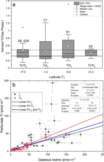
Figure 6 shows that the average and range of the TI/Iy and TI/TIy ratios are very similar and do not show a dependence on geographical location beyond the range of variability. The proximity of the TI/Iy and TI/TIy ratios in the tropics and midlatitudes can be expected, considering that the contribution of GOI to TIy at those locations, as well as throughout the tropical free troposphere, is expected to be ∼20% (Koenig et al., 2020; Pra- dos-Roman et al., 2015; Saiz-Lopez et al., 2014). The relative invariance of the aerosol to gas phase ratio may be used to scale the TIy or Iy computed by CAM-Chem to make them comparable to the observations in absolute terms.

Figure 6a indicates that the particulate TI versus gaseous iodine ratio takes values between ∼0.3 (error-weighted average of the 56 datapoints) and ∼0.5 (the unweighted average in Figure 6a). Therefore, the gaseous iodine concentration is on average between 2 and 3 times higher than the iodine concentration in aerosol. A caveat to this result is that 54 out of the 56 datapoints in Figure 6a were measured between 1963 and 1979, which could affect the Iy to TI conversion for more recent periods of time if the ratio has changed significantly since then. Independent fits of the Iy and TIy scatterplots (Figure 6b) give statistically significant slopes of 0.27 ± 0.07 and 0.42 ± 0.07, respectively, with intercepts not significantly different from zero at 95% confidence level. The TI versus Iy regression alone yields a poor correlation coef- ficient. A global fit of TI versus both Iy and TIy data yields an intermediate slope of 0.32 ± 0.04, again with an intercept statistically indistinguishable from zero.

3.3. Spatial and Temporal Variability of Aerosol Iodine 3.3.1. TI Statistics by Campaign

Table 4 lists descriptive statistics of the field campaigns described in Tables 2 and 3. These statistics (arithmetic mean, standard deviation, geometric mean, geometric standard deviation, minimum, first quartile, median, third quartile, and maximum) have been calculated from the individual sample data available. For those campaigns for which the data could not be retrieved, the statistics reported in the corresponding paper are included in the table (campaigns highlighted in bold font). In the particular case of S30, a monthly box and whisker plot with medians, quantiles, maximum, and minimum is provided in the original publication, from which the maximum and minimum values of the full campaign are given in the table. The median of Figure 5. Latitudinal dependence of TI. (a) Data points with error bars

(for samples the error bars represent the analytical uncertainty, for full campaign averages the error bars are not shown). (b) Campaign averages with error bars (standard deviation of each campaign). The data of each cruise are shown binned into 10° zonal band averages. TI, total iodine.

(12)

the campaign is calculated as the median of the monthly medians, and the arithmetic mean is estimated for plotting purposes as the average of the monthly maxima and minima (estimated values are given in italics).

3.3.2. Latitudinal Dependence

Figure 5a with all the datapoints and Figure 5b with the campaign averages show a clear dependence of TI on latitude. To highlight these features, Figure 7a shows the complete bulk aerosol TI data set plotted versus 10°

wide latitudinal bands in box and whisker fashion. All statistics show a clear latitudinal dependence, with TI peaking in the tropical regions and decreasing toward the poles, although there is a hemispheric asymmetry where the values in the NH tend to be higher than in the Southern Hem- isphere (SH). As a note of caution, there is a heavy hemispheric sampling imbalance, with the majority of the samples taken in the NH (n = 208 in the SH vs. n = 7,586 in the NH). There are many more outliers in the NH, most of which result from the recent measurements in Mace Head (S32) and the northern Atlantic (C8), as well as from observations in the Arctic Ocean (C13). The inclusion of high-altitude stations (S1b–d, S17), data possibly affected by new particle formation (C8 and S32) and data potentially affected by recent loss of sea ice (C13) may distort the long- term latitudinal dependence of aerosol TI.

Figure 7b shows the latitudinal dependence of the TI data without the C8, S32, S1b–d, S16, and the Arctic transect of C13. This increases the average at 25° (by removing the high-altitude low values at Izaña) and decreases the average at 55° and 75° (by removing high values in the northern Atlantic and the Arctic). Thus, besides the known lower values at high altitude, note that some recent NH TI data appear to be enhanced with respect to the historic record (see below).

A caveat to the analysis performed in Figure 7 is that for those zonal bands where most of the data correspond to one or two stations (15°, 25°, 35°, 55°, and 85°), the corresponding zonal average is totally dominated by these stations (Figure 5a). An alternative way of analyzing these data is grouping the campaign averages (Figure 5b) in zonal bands (Fig- ure S2). By comparing Figures 7 and S1, it can be seen that the latitudinal dependence of sample and campaign zonal averages of TI is very similar, supporting the statistical analysis performed here.

3.3.3. Longitudinal Dependence

Figures 8 and S3 show the longitudinal dependence of TI in bulk aerosol for datapoints and campaign averages, respectively. Within the tropics, the highest concentrations are observed in the Atlantic. At midlatitudes in the NH, the data acquired during the 2006 MAP campaign at Mace Head (C8 and S32) enhance the average at −15° longitude (Atlantic). After screening the C8 and S32 data, likely affected by coastal and open ocean new particle formation (O’Dowd et al., 2002, 2010), it appears that the highest average concentration in the NH midlatitudes occurs in South- East Asia (135° longitude). In the SH, the TI concentrations are somewhat lower in the Indian Ocean compared to those in the Atlantic Ocean.

3.3.4. Seasonal Variation

Figure S4 shows the monthly climatology of TI in bulk aerosol for six different latitudinal bands. For midlatitudes and tropics, the climatologies are also divided into Atlantic and Pacific. The seasonal variability in the Arctic and in Antarctica is similar, presenting equinoctial maxima, with the spring maximum showing enhanced values. At Atlantic and Pacific NH midlatitudes, aerosol iodine does not show a discernible seasonal variation, but there are hints of seasonal cycles in the NH tropics. The TI data for SH low latitudes Figure 6. (a) Box and whiskers plot showing statistics of TI/TIy and TI/

Iy ratios at four latitudes (for the cruise C1, the average latitude is shown).

IQR, interquartile range. The horizontal dashed line shows the unweighted average of the 56 ratios available. (b) Linear regressions with instrumental error in both coordinates of measured particulate TI versus measured gas-phase iodine (TIy, Iy, and both). The horizontal solid line in panel (a) corresponds to the slope of the concatenated fit (0.32), which is roughly the same as the error-weighted average of the 56 points. TI, total iodine.

(13)

# N Mean SD Geo mean Geo SD Min Q1 Median Q3 Max

C1 24 46.6 30.7 39.1 1.8 15.8 23.6 39.4 51.2 134.0

C2 17 7.5 7.2 7.5 2.3

C3 1 30.6

C4 28 41.3 30.4 32.5 2.0 12.7 18.2 25.8 59.1 118.4

C5 44 39.1 15.9 36.1 1.5 14.5 28.6 38.2 46.0 81.0

C6 22 33.5 14.5 31.1 1.5 14.8 24.0 30.9 36.8 77.9

C7 57 16.2 15.8 10.9 2.4 2.4 5.0 9.4 23.4 68.7

C8 33 410.7 339.7 281.6 2.6 31.9 149.8 334.8 658.3 1,511.0

C9 14 13.6 3.8 13.1 1.3 7.8 11.6 13.1 16.5 21.7

C10 14 57.7 23.9 53.8 1.5 33.8 40.7 51.5 66.2 112.5

C11 17 48.5 21.4 44.0 1.6 16.0 33.1 47.6 57.3 97.1

C12 8 33.4 12.5 31.4 1.5 17.8 25.1 29.8 43.9 52.0

C13 28 88.3 95.9 61.3 2.2 20.0 30.5 53.5 103.0 443.0

C14 13 20.6 12.0 17.4 1.9 6.0 10.7 14.3 28.4 42.7

C15 11 7.9 2.6 7.5 1.4 5.0 6.0 7.0 10.0 13.0

C16 24 58.5 38.9 44.9 2.2 7.0 24.0 53.5 90.5 134.0

C17 33 42.0 20.7 38.1 1.5 17.8 28.8 39.8 46.7 105.8

C18 11 15.2 3.9 14.8 1.3 11.0 12.5 13.6 17.9 22.3

C19 10 28.1 8.1 27.1 1.3 17.8 22.5 26.2 33.7 40.9

S1a 5 63.8 73.8 42.1 2.6 14.9 25.9 39.5 44.6 194.1

S1b-d 4 15.3 3.7 14.9 1.3 10.4 12.3 16.2 18.2 18.3

S2 10 36.5 18.6 32.3 1.7 13.8 23.2 34.7 45.7 72.5

S3 23 11.8 18.1 7.0 2.4 2.4 3.7 6.7 10.2 74.1

S4 8 13.4 9.0 11.4 1.8 6.9 7.2 9.3 17.2 32.6

S5 11 19.7 8.3 18.4 1.5 11.0 12.6 18.9 22.9 41.0

S6 19 7.5 3.3 7.0 1.5 4.0 5.0 6.7 9.5 14.2

S7 287 14.2 9.5

S8^b 135 4.9 2.9 3.9 2.3 0.1 2.8 4.6 6.3 13.6

S9 27 26.0 15.8 21.1 2.0 5.3 12.6 22.9 37.0 62.3

S10^c 110 7.6 4.7 6.4 1.8 0.9 4.1 6.5 10.0 31.5

S11 1,234 3.4 2.8 2.6 2.2 0.1 1.6 2.8 4.5 35.1

S12a 7 13.0 10.0 12.6 2.0

S12b 4 9.0 1.0 8.7 1.1

S13 11 8.7 4.1

S14 9 52.4 30.1 44.4 1.9 13.4 36.2 44.9 59.1 100.1

S15 1,308 20.0 15.3 16.4 1.9 0.5 10.8 16.3 24.2 224.6

S16 2,750 42.7 26.5 36.1 1.8 2.1 24.6 36.5 54.0 231.7

S17 905 14.9 138.7 7.3 2.2 1.5 4.4 6.4 11.0 4,160.8

S18 436 22.3 29.2 14.9 2.4 1.3 8.4 14.0 26.2 424.0

S19 13 12.1 6.2 10.4 1.9 2.4 10.2 11.0 15.0 26.8

S20a 35 10.2 4.2

S20b 35 5.9 2.1

S21 12 6.4 3.7 4.9 2.5 0.4 3.6 6.0 8.6 13.8

Table 4

Statistics of Total Iodine (TI) in Bulk Aerosol (Units: pmol m⁻³)^a

(14)

and midlatitudes are too sparse to draw any conclusions. It must be pointed out, nevertheless, that only a few campaigns at specific sites report year-long measurements, which can yield a proper climatology.

Thus, averaging of dissimilar data sets with sparse monthly coverage in different years and at widespread locations may result in unrealistic TI climatologies. This is especially true considering that local weather seasonal cycles as well as local iodine sources may vary significantly within the same zonal and meridional band. For example, the Antarctic seasonal variation was recorded almost entirely in Neumayer II between January 2007 and January 2008, while only a few measurements in spring and summer were carried out at Filchner station (S29) and McMurdo (S6). Thus, the “Antarctic” TI seasonal cycle plotted in Figure S4 is mainly the cycle at Neumayer II, which may not be representative of the entire Antarctic coast. This is also the case for other regions: the climatology in the NH tropical Atlantic is dominated by the multiyear AEROCE measurements at Barbados (S16), while the year-long data set recorded at Hong Kong (S30) determines the monthly statistics in the tropical Pacific. Additional data from other campaigns with incomplete coverage only distort the local cycles without bringing in additional information. For this reason, we plot in Figure 9 the monthly climatologies for each of the nine stations at sea level (S8, S10, S11, S15, S16, S18, S19, S30, and S33) where year-long measurements of TI or TSI have been carried out (the TI monthly climatology at Izaña, in the free troposphere, is also available). Seasonal cycles can be observed at Mould Bay (S8), Alert (S11), and Neumayer II (S33), with a similar double peak profile as mentioned above. The lack of a clear seasonal variation at Igloolik compared to Mould Bay and Alert was already noticed by Sturges and Barrie (1988). Measurements at midlatitude stations (S15, S18, and S19) do not show a clear seasonal variation. Note that the data acquired during the MAP campaign in June–July 2006 at Mace Head (S32) are anomalously high compared to the June and July averages of the AEROCE campaign between 1989 and 1994 (S18). In the NH tropics, Barbados (S16) and Hong Kong (S30) show cycles which are mutually out

Table 4 Continued

# N Mean SD Geo mean Geo SD Min Q1 Median Q3 Max

S22 50 51.2 22.8 46.9 1.5 19.1 35.9 42.9 63.4 134.0

S23 29 27.3 18.3 22.8 1.8 7.5 13.9 23.8 37.8 97.7

S24 8 28.2 11.0 26.3 1.5 15.0 18.6 28.0 36.3 44.8

S25 6 67.9 15.3 66.7 1.2 54.2 61.1 63.2 67.9 97.7

S26 37 20.3 8.9 18.9 1.4 9.6 15.2 19.1 22.9 56.1

S27 15 20.7 12.0 18.0 1.7 6.5 13.2 18.0 25.1 55.0

S28 85 6.0 2.5 5.6 1.5 2.1 4.0 6.0 7.5 16.3

S29 2 5.0 1.6 3.9 6.2

S30 114 23.0 14.0 1.8 21.9 91.3

S31 16 23.9 12.0 20.7 1.8 5.2 13.5 23.7 32.0 50.4

S32 45 563.1 596.6 403.0 2.1 66.7 247.7 335.1 601.5 3,041.6

S33 56 5.0 2.5 4.5 1.5 2.6 3.3 4.0 5.7 15.0

S34 3 41.3 26.7 33.8 2.3 13.0 13.0 45.0 66.0 66.0

S35 8 14.1 4.1 13.5 1.4 8.2 10.6 14.7 17.3 19.5

S36 3 82.4 70.3 64.6 2.3 31.1 31.1 53.5 162.5 162.5

aCampaigns for which only statistics have been published and for which the original data could not be retrieved are highlighted in bold font. For the rest of the campaigns, the statistics have been calculated form the available datapoints.

SD, Geo Mean, Geo SD, Min, Q1, Q3, and Max are, respectively, the standard deviation, the geometric mean, the geometric standard deviation, the minimum, the first quartile, the third quartile, and the maximum. Values in italics:

the arithmetic mean and standard deviation have been estimated for plotting purposes, because the original papers only report the geometric mean and geometric standard deviation. ^cIgloolik: the arithmetic mean and standard deviation of a subset of 67 measurements reported in the original paper are 8.1 ± 5.1 pmol m⁻³. TI statistics for the full data set were not reported (Sturges & Barrie, 1988).

bMould Bay: the arithmetic mean and standard deviation of a subset of 67 measurements reported in the original paper are 4.0 ± 3.2 pmol m⁻³. TI statistics for the full data set were not reported (Sturges & Barrie, 1988).

(15)

of phase (the July maximum of S16 coincides with a minimum of S30).

Although S30 was a 1-year campaign, the high-frequency measurements during S22 (September–November) appear to confirm an annual cycle peaking toward the end of the year.

3.3.5. Long-Term Trends

Box and whiskers plots of TI measurements in the NH grouped by year are shown in Figure 10 (the SH data are too sparse to perform a long-term trend analysis). The long-term series in Figure 10 suggest that increases in TI may have occurred between 1963 and 2010. However, both linear and exponential (i.e., apparent linear fitting of the semilogarithmic scatter plot) unweighted fits of the annual averages indicate that the slopes are not significantly different from zero at 95% confidence level. Thus, the NH data are compatible both with decreasing and increasing trends as indicated by the confidence bands in Figure 10. As a result of the meth- odological change around year 2000, when most research turned to soluble iodine measurements instead of TI, the long-term trends are critically dependent on the TSI–TI scaling.

4. Discussion

4.1. Latitudinal Dependence

The latitudinal profile of aerosol TI is reminiscent of the sea water I⁻ profile (Chance et al., 2019), showing high concentrations in low-latitude warm waters and low iodide concentrations at high latitudes in seasonal- ly overturning cold waters (Figure S5b). Thus, aerosol iodine likely tracks the emission fluxes of the dominant iodine source, which is the I⁻ + O3

reaction in the ocean surface (Carpenter et al., 2013). The hemispheric asymmetry likely results from the higher abundance of anthropogenic O3

in the NH (Figure S5c) (Prados-Roman et al., 2015).

The ratio TI/TSI is key to homogenize the most recent cruise data and make it directly comparable to the TI measurements. Although speciation will be discussed in a follow-up work, it is worth mentioning here that the TSI group dominates TI almost everywhere except in the high latitudes, where there is some evidence of enhanced NSI (Figure 2). In the particular case of the new data set from Neumayer II (S33), TSI values are low and comparable to the intercept of Equation 1. Thus, the TI values obtained with Equation 1 for S33 result in a relatively high TI/TSI ratio (S33 average of 2.9 ± 1.1). This is consistent with the higher values of TI/TSI at high latitudes shown in Figure 2a (TI/TSI = 2.4 ± 2.3 at high latitudes, TI/TSI = 1.6 ± 0.7 at middle and low latitudes inside the black box in Figure 2a), but it must be kept in mind that TI/TSI values closer to 1 are also registered in a full campaign at high latitudes (C13), and therefore Equation 1 may overestimate TI at Neumayer.

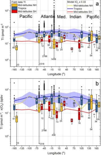
Because of the large scatter in the aerosol iodine/gas-phase iodine ratios (Section 3.2), we have chosen a range of scaling factors (0.3–0.5) to convert modeled gas-phase TIy and Iy into values comparable to aerosol TI. The ranges of modeled aerosol TI proxies obtained in this way are encompassed by the thin red and blue lines in Figure 7, while the central thick red and blue lines are obtained using the average aerosol iodine/

gas-phase iodine scaling factor. Note that modeled gas-phase TIy and Iy have also a variability range (red and blue shaded regions in Figure 7a). The agreement between the REF-C1 simulated TIy and Iy scaled averages is good at low latitudes and midlatitudes, where TI ∼ I. At high latitudes, a larger fraction of TI is in the Figure 7. Latitudinal dependence of bulk aerosol total iodine. The box

and whiskers statistics of available datapoints correspond to 10° zonal bands. The numbers below each whisker indicate the datapoints within each zonal band. (a) TI statistics of all campaigns listed in Tables 1 and 2.

Circles and triangles indicate the average, maximum, and minimum Iy

(blue symbols) and TIy (red symbols) measured in five campaigns. Solid blue and red lines and shaded areas indicate the 1950–2010 average and ranges of Iy and TIy, respectively, computed with CAM-Chem. (b) As panel (a), but excluding high-altitude data (Izaña and Mauna Loa observatories), data potentially affected by new particle formation (North Atlantic and Mace Head MAP 2006 measurements, Chinese coast measurements) and Arctic cruises potentially affected by sea ice loss (samples of the third China Arctic Research Expedition collected in the Arctic Ocean). Panel (b) also includes the simulated 1950–2010 averages of Iy and TIy scaled by factors 0.5, 0.42, and 0.33, as indicated by the analysis in Figure 6. Note the different vertical scale in the two panels. TI, total iodine; CAM-Chem, Community Atmospheric Model with chemistry.

(16)

form of GOI, which explains why scaled TIy overestimates TI. By contrast, scaled Iy underestimates TI (see Figure 7). Here, it should be noted that the ocean iodide parameterization used in CAM-Chem results in a less pronounced latitudinal shape and lower values than other iodide data sets based on observations and/or machine learning studies (see Figure 2 in Carpenter et al. [2021]), which certainly affect the modeled Iy levels.

Additionally, since the polar module was not run in the REF-C1 simulation, ice sources of inorganic iodine are not accounted for, and therefore the model produces less Iy (Fernandez et al., 2019), which explains why the scaled Iy curves lie below the TI observations.

4.2. Longitudinal Dependence

In the tropics, TI is enhanced in the Atlantic, which results from a combination of high biogenic activity in the equatorial Atlantic (especially close to the Gulf of Guinea, as shown by the R/V Capricorne observations) and the zonal wave-one pattern of tropical tropospheric O3 (Thompson et al., 2003), which peaks in the Atlantic and enhances the inorganic source. A caveat is the lack of measurements in the tropical eastern Pacif- ic. The modeled Iy has a similar longitudinal dependence than the TI statistics, although smoother and with a less pronounced Pacific minimum (Figure 8). However, note that due to the local SST and iodide enhance- ments in the Maritime Continent, the oceanic iodide flux over this region where most of the Pacific measurements were performed can be more than 2 times larger with respect to most of the central Pacific. Indeed, Figure 4 shows that modeled surface Iy is much lower in the tropical central and eastern Pacific compared to the western Pacific. The longitudinal variation of seawater iodide in the tropics (Chance et al., 2019) shows a minimum between in the Atlantic between 40°W and 15°E, which is not present in TI (Figures S6a and S6b). The tropical Atlantic TI maximum is probably a result of a higher ozone concentration in that region. Note that CAM-Chem reproduces correctly the wave-one longitudinal dependence of tropospheric and surface O3 in the tropics (Figure S6c).

TI shows a relative maximum in the NH western Pacific, most likely as a result of O3 pollution outflowing from China, perhaps with an additional contribution of biogenic iodine source gases resulting from extensive al- gae farming. CAM-Chem also predicts a local maximum of TIy (Figure 4) and Iy (Figure 8), as well as of O3 (Prados-Roman et al., 2015) at those latitudes. The oceanic iodine gas source parameterization implemented in CAM-Chem is based on a SST-dependent iodide field (Figures S5 and S6) and thus it is not capable of capturing regional changes in oceanic bio- chemistry, which are likely to have an impact on atmospheric chemistry over the different oceans. Indeed, Inamdar et al. (2020) recently showed that many region-specific parameters, such as ocean salinity and revers- ing wind patterns, are required to capture the sea surface iodide distribution over the Indian Ocean.

The high average Iy values predicted by the model at midlatitudes in the NH for the 15° and 45° meridional bands shown in Figure 8 result from the high concentrations above the Mediterranean Sea (Figure 4). Al- though the concentration of I⁻ in Mediterranean seawater is not particularly high (Chance et al., 2019), the Mediterranean basin shows elevated ozone concentrations, which are expected to significantly enhance I2

and HOI emissions (Prados-Roman et al., 2015). The three campaigns in the 15° meridional band at midlatitudes took place at the top latitude end (Scandinavia) and show lower TI concentrations than the average model prediction, although in agreement with the model predictions for those locations (Figure 4).

Figure 8. Longitudinal dependence of bulk aerosol total iodine. The box and whiskers statistics of available datapoints correspond to 30°

meridional bands. The number of datapoints within each meridional band appears under the corresponding box. Box and whiskers statistics as in previous figures. The red and yellow boxes correspond to respectively to SH midlatitudes (60°S–25°S) and NH midlatitudes (25°N–60°N), and the blue boxes to low latitudes (25°S–25°N). (a) All midlatitude and low-latitude campaigns listed in Tables 1 and 2. (b) As panel (a) but excluding high-altitude data (Izaña and Mauna Loa observatories) and data potentially affected by new particle formation (North Atlantic and Mace Head MAP 2006 measurements). Both panels show the Iy 1950–2010 average computed by the model for the corresponding latitudinal band, scaled by a factor of 0.33. The blue shaded region indicates the span of the Iy range (1950–2010) in the tropics. Note the different vertical scale in the two panels. SH, Southern Hemisphere; NH, Northern Hemisphere.

(17)

Sherwen, Evans, Spracklen, et al. (2016) implemented in GEOS-Chem the same online oceanic iodine source that we use in CAM-Chem and compared their modeling results with a subset of cruise TSI measurements. Their global maps of modeled TI suggest latitudinal and longitudinal variations that are consistent with the spatial variations demonstrated by the TI field data compiled in the present work. The average TI absolute values modeled by GEOS-Chem are consistent with the TI field observations and the agreement with the subset of TSI measurements considered by Sherwen et al. improves if Equation 1 is used to convert observed TSI into TI.

4.3. Seasonal Variation

The seasonal profiles of TI in the Arctic (Mould Bay and Alert) and in Antarctica (Neumayer II) are similar, showing equinoctial maxima with an absolute maximum in the polar spring (Figure 9). The seasonal variation at Igloolik is less clear. While the TI seasonal profiles in the Arctic have been discussed previously, the TI Antarctic profile is reported in this work for the first time. This double seasonal peak is also observed in year-long IO measurements at Halley (Antarctica) (Saiz-Lopez et al., 2007) and is well captured by the Figure 9. Bulk aerosol TI climatologies in nine stations. The box and whiskers statistics are defined as in previous figures. In panel (f), monthly averages, maxima, and minima of a limited data set acquired at Ibaraki (S19) are shown. In panel (h), the box and whiskers plot for S30 shown in the corresponding reference is reproduced (no mean reported, only median values), with the triangles indicating maxima and minima. Panel (h) also incorporates PEM WEST A measurements at Hong Kong (S22) with a high sampling frequency but just for 3 months. The solid red lines correspond to the REF-C1 climatologies of scaled Iy for the 1950–2010 period (error bars indicate in this case 1σ variability within that period), while the polar module Iy climatology for year 2000 is shown in blue. A scaling factor of TI/Iy = 0.33 is used in all cases. TI, total iodine.