Quantification of Ocean Heat Uptake from Changes in Atmospheric O

Supplementary Information for

Quantification of Ocean Heat Uptake from Changes in Atmospheric O

and CO

Composition

L. Resplandy¹*, R. Keeling², Y. Eddebar², M. Brooks², R. Wang³, L. Bopp³, M. C. Long⁴, J. P. Dunne⁵, W. Koeve⁶, A. Oschlies⁶

1Department of Geosciences and Princeton Environmental Institute, Princeton University, Princeton, USA.

2Scripps Institution of Oceanography, University of California San Diego, La Jolla, USA.

3Department of Environmental Science and Engineering, Fudan University, Shanghai, 200433 China.

4Laboratoire de Météorologie Dynamique / Institut Pierre Simon Laplace, CNRS / ENS / X / UPMC, Département de Géosciences, Ecole Normale Supérieure, Paris.

5National Center for Atmospheric Research, Boulder, USA.

6NOAA, Geophysical Fluid Dynamics Laboratory, Princeton, USA.

7GEOMAR Helmholtz Centre for Ocean Research, Kiel, Germany.

*Correspondence to: laurer@princeton.edu.

This PDF file includes:

Figs. S1 to S4

Tables S1 to S6

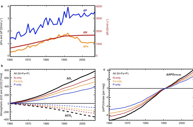
Figure S1. Effects of anthropogenic aerosols on APO. a. Anomaly, relative to 1850 levels, in deposition of atmospheric anthropogenic aerosols (N, P and Fe) at the air–sea interface between 1960 and 2007, derived from model simulations with and without aerosols ²³. b. Impact of aerosol

eutrophication on atmospheric O2 (solid lines) and CO2 (dashed lines) for all aerosols (black lines) and for each aerosol taken individually (coloured lines). c, Overall impact of aerosol eutrophication

on ΔAPOClimate referenced to the first year that has observations (1991).

1960 1970 1980 1990 2000

0 1 2 3 4

ΔFe and ΔP [Gmol y-1]

0 1000 2000 3000 4000

ΔN [Gmol y-1]

1960 1970 1980 1990 2000

-400 -200 0 200 400 600 800

Atmospheric ΔO2 and ΔCO2 [Tmol] ΔAPOclimate [per meg]

ΔFe ΔN ΔP

ΔO₂

ΔCO₂ a

b

c

Fe-only N-only P-only All (N+Fe+P)

Fe-only N-only P-only

All (N+Fe+P) ΔAPOClimate

1960 1970 1980 1990 2000

-6 -4 -2 0 2 4

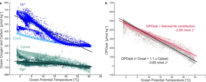
Figure S2. Solubility-driven changes in ocean oxygen and carbon concentrations. a. Ocean observations of O2*, O2sat, Cpi* and Cpisat as a function of potential temperature in the GLODAPv2 database ⁴⁹. b. OPO sat ( = O2sat + 1.05 Cpisat, in grey) and the expected effects on APO owing to the combined effects of OPO sat and the thermal exchanges of N2 ( = O2sat + 1.05 Cpisat – XO2 / XN2 [N2 – mean(N2)], in red). For clarity only 16 ×10³ points randomly picked out of the 78,456 data points available are shown for each variable. Note that very low values of O₂^* (around 450 µmol kg^-1) at low temperature (less than 10 °C) correspond to data collected in the Arctic Ocean, where phosphate concentrations (used for O2* calculation) are comparatively lower than in other cold ocean regions.

Low O2* values in the Arctic explain the relatively low values of OPO shown in Fig. S3a at temperatures below 10 °C.

0 5 10 15 20 25 30 35

−200

−100 0 100 200 300 400 500 600 700 800

Ocean Oxygen and Carbon [µmol kg-1]

Ocean Potential Temperature [°C]

O2*

O2sat

Cpi*

Cpisat

OPOsat (= O2sat + 1.1 x Cpisat) -3.65 nmol J^-1

OPOsat + thermal N2 contribution -2.95 nmol J^-1

OPOsat [µmol kg-1]

Ocean Potential Temperature [°C]

0 5 10 15 20 25 30 35

−200

a b

0 5 10 15 20 25 30 35

−100 0 100 200 300 400 500 600 700

−

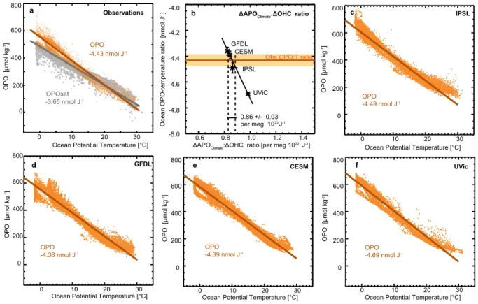
Figure S3. Link between OPO, APOClimate and ocean heat.a, c–f, OPO concentrations (yellow) and OPO concentrations at saturation based on O2 and CO2 solubility (OPOsat, grey) as a function of ocean

temperature in the GLODAPv2 database ⁴⁹ (a) and four Earth-system models (IPSL, GFDL, CESM and UVic; c–f). Slopes give the OPO-to-temperature ratios in nmol J^-1. b. The link between ΔAPOClimate and changes in ocean heat content (that is, ΔAPOClimate-to-ΔOHC ratio) in the four models is tied to their OPO-to-temperature ratios and can be constrained using the observed OPO-to-temperature of 4.43 nmol J−1 (vertical dashed lines). To avoid visual saturation, only 16,000 points, picked randomly, are shown for OPO.

ΔAPO_Climate:ΔOHC ratio [per meg 10²² J^-1] Ocean OPO-temperature ratio [nmol J-1]

OPO [µmol kg-1]

Ocean Potential Temperature [°C]

0 400 800

200 600

0 10 20 30

Ocean Potential Temperature [°C]

a b

e

0 10 20 30

0 200 400 600 800

0 10 20 30

0 200 400 600 800

0 10 20 30

0 200 400 600 800

0 10 20 30

0 200 400 600 800

OPO -4.49 nmol J^-1

OPO -4.36 nmol J^-1

OPO

-4.39 nmol J^-1 OPO

-4.69 nmol J^-1

Ocean Potential Temperature [°C]

Ocean Potential Temperature [°C]

Ocean Potential Temperature [°C]

OPO [µmol kg-1]

OPO [µmol kg-1] OPO [µmol kg-1] OPO [µmol kg-1]

0.6 0.8 1.0 1.2 1.4

-5.0 -4.8 -4.6 -4.4 -4.2

-4.0 ΔAPO_Climate:ΔOHC ratio

Observations

d CESM f UVic

IPSL

GFDL

c

Obs OPO:T ratio

0.86 +/- 0.03 per meg 10²²J^-1

IPSL GFDL

UViC CESM OPO

-4.43 nmol J^-1

OPOsat -3.65 nmol J^-1

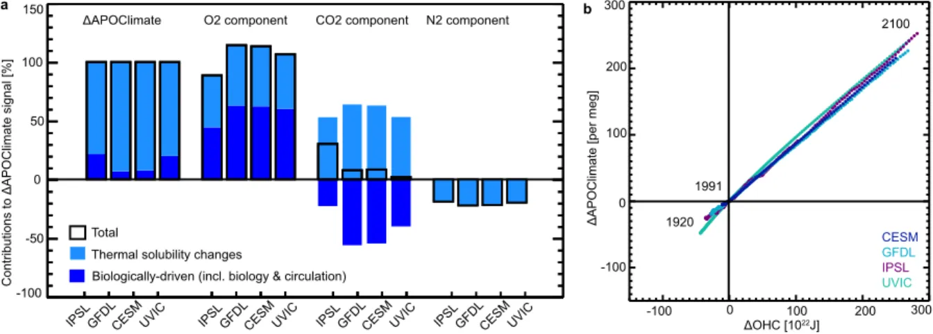
Figure S4. Changes in APOClimate (ΔAPOClimate) and ocean heat content (ΔOHC) in four Earth- system models. A. Simulated ΔAPOClimate (black outlines) are decomposed into the contributions (percentage of total) from changes in ocean thermal saturation (light blue) and biologically driven changes (dark blue), the latter including changes in photosynthesis/respiration and changes in ocean circulation that transport and mix gradients of biological origin. For each model, ΔAPOClimate is further decomposed into its O2, CO2 and N2 components—that is, how much of ΔAPOClimate is explained by changes in O2, CO2 and N2 air–sea fluxes due to ocean saturation changes and biologically driven

changes. b. Model ΔAPOClimate-to-ΔOHC ratios over the 180 years of simulation (referenced to year 1991) in per meg per 10²² J units are: 0.85 ± 0.01 (CESM), 0.83 ± 0.01 (GFDL), 0.89 ± 0.03 (IPSL) and 0.99 ± 0.02 (UVic).

ΔOHC [10²²J]

ΔAPOClimate [per meg] 1920

2100

1991

Contributions to ΔAPOClimate signal [%]

Biologically-driven (incl. biology & circulation) Total

Thermal solubility changes

IPS L

GFD L

CESM UVIC -100

-50 0 50 100

150 ΔAPOClimate O2 component CO2 component N2 component

IPS L

GFD L

CESM UVIC IPS

L GFD

L

CESM UVIC IPS L

GFD L

CESM UVIC

a b

-100 0

100 200 300

-100 100 200 300

CESM GFDL IPSL UVIC 0

Table S1. Sources of the hydrographic databased estimates of global changes in ocean heat

content (ΔOHC) used in Fig. 1.

Label in Fig 1 0 to 2000 m depth range

2000 to 6000 m depth range

PMEL Ref. 6 Ref. 7

MRI Ref. 5 Ref. 7

NCEI Update of ref. 47 Ref. 7

CHEN Ref. 8 Ref. 7

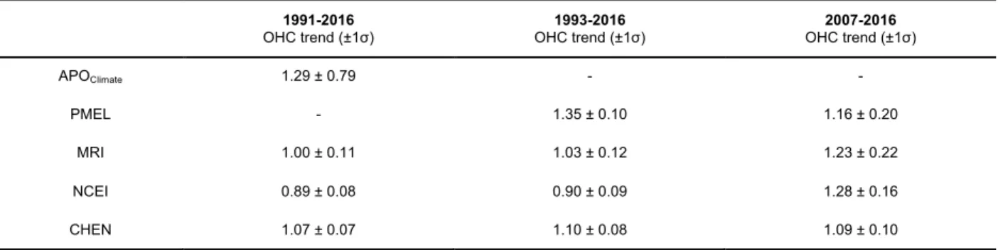
Table S2. Linear trends in ocean heat content.

1991-2016

OHC trend (±1σ) 1993-2016

OHC trend (±1σ) 2007-2016

OHC trend (±1σ)

APOClimate 1.29 ± 0.79 - -

PMEL - 1.35 ± 0.10 1.16 ± 0.20

MRI 1.00 ± 0.11 1.03 ± 0.12 1.23 ± 0.22

NCEI 0.89 ± 0.08 0.90 ± 0.09 1.28 ± 0.16

CHEN 1.07 ± 0.07 1.10 ± 0.08 1.09 ± 0.10

Units are 10²² J yr⁻¹. Trends and ±1σ uncertainty ranges are given for hydrographic (in situ temperature) and atmospheric (APO) data over the depth range 0–6,000 m. See Table S1 for literature sources of estimates.

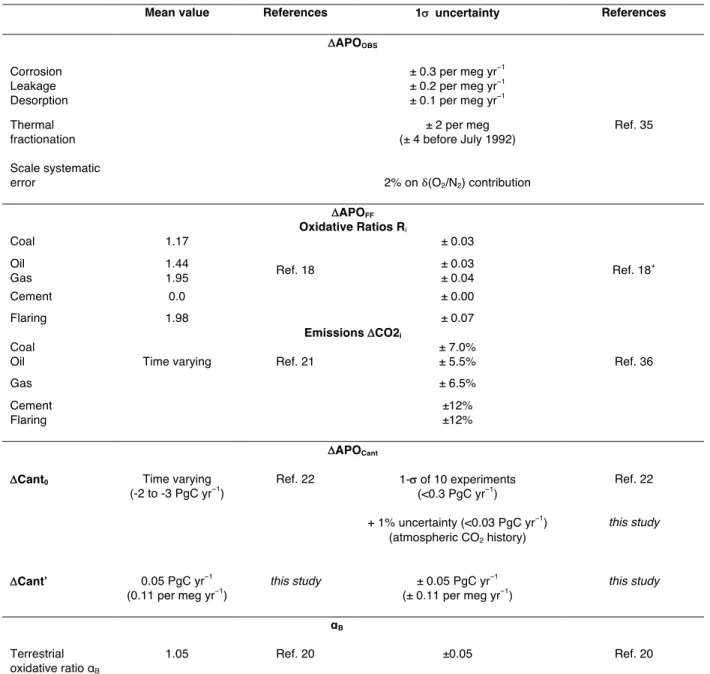
Table S3. Contributions to DAPOOBS, DAPOFF and DAPOCant and associated uncertainties (±1σ) during the observation period (1991 to 2016).

Mean value References 1s uncertainty References

DAPOOBS

Corrosion ± 0.3 per meg yr⁻¹

Leakage ± 0.2 per meg yr⁻¹

Desorption ± 0.1 per meg yr⁻¹

Thermal fractionation

± 2 per meg (± 4 before July 1992)

Ref. 35

Scale systematic

error 2% on δ(O2/N2) contribution

DAPOFF

Oxidative Ratios Ri

Coal 1.17

Ref. 18

± 0.03

Ref. 18⁺

Oil 1.44 ± 0.03

Gas 1.95 ± 0.04

Cement 0.0 ± 0.00

Flaring 1.98 ± 0.07

Emissions DCO2i

Coal

Time varying Ref. 21

± 7.0%

Ref. 36

Oil ± 5.5%

Gas ± 6.5%

Cement ±12%

Flaring ±12%

DAPOCant

DCant0 Time varying (-2 to -3 PgC yr⁻¹)

Ref. 22 1-s of 10 experiments (<0.3 PgC yr⁻¹) + 1% uncertainty (<0.03 PgC yr⁻¹)

(atmospheric CO2 history)

Ref. 22

this study

DCant’ 0.05 PgC yr⁻¹ (0.11 per meg yr⁻¹)

this study ± 0.05 PgC yr⁻¹

(± 0.11 per meg yr⁻¹)

this study

αB

Terrestrial oxidative ratio αB

1.05 Ref. 20 ±0.05 Ref. 20

+ Uncertainties in fossil-fuel oxidative ratios are ultimately from Keeling, 1988, Developing an interferometric oxygen analyzer for precise measurements of the atmospheric O2 mole fraction, PhD thesis, Harvard University. We interpret these as 1-sigma uncertainties despite language in Keeling (1988) that suggest they may be 90% confidence intervals because they are based on 1- sigma spread across fuels.

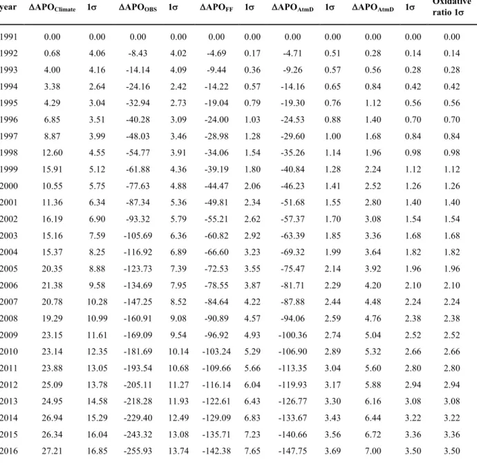
Table S4. Temporal evolution of the cumulative contributions to global APO changes and their 1σ uncertainties.

year DAPOClimate 1s DAPOOBS 1s DAPOFF 1s DAPOAtmD 1s DAPOAtmD 1s Oxidative ratio 1s

1991 0.00 0.00 0.00 0.00 0.00 0.00 0.00 0.00 0.00 0.00 0.00

1992 0.68 4.06 -8.43 4.02 -4.69 0.17 -4.71 0.51 0.28 0.14 0.14

1993 4.00 4.16 -14.14 4.09 -9.44 0.36 -9.26 0.57 0.56 0.28 0.28

1994 3.38 2.64 -24.16 2.42 -14.22 0.57 -14.16 0.65 0.84 0.42 0.42

1995 4.29 3.04 -32.94 2.73 -19.04 0.79 -19.30 0.76 1.12 0.56 0.56

1996 6.85 3.51 -40.28 3.09 -24.00 1.03 -24.53 0.88 1.40 0.70 0.70

1997 8.87 3.99 -48.03 3.46 -28.98 1.28 -29.60 1.00 1.68 0.84 0.84

1998 12.60 4.55 -54.77 3.91 -34.06 1.54 -35.26 1.14 1.96 0.98 0.98

1999 15.91 5.12 -61.88 4.36 -39.19 1.80 -40.84 1.28 2.24 1.12 1.12

2000 10.55 5.75 -77.63 4.88 -44.47 2.06 -46.23 1.41 2.52 1.26 1.26

2001 11.36 6.34 -87.34 5.36 -49.81 2.34 -51.68 1.55 2.80 1.40 1.40

2002 16.19 6.90 -93.32 5.79 -55.21 2.62 -57.37 1.70 3.08 1.54 1.54

2003 15.16 7.59 -105.69 6.36 -60.82 2.92 -63.39 1.85 3.36 1.68 1.68

2004 15.37 8.25 -116.92 6.89 -66.60 3.23 -69.32 1.99 3.64 1.82 1.82

2005 20.35 8.88 -123.73 7.39 -72.53 3.55 -75.47 2.14 3.92 1.96 1.96

2006 21.38 9.58 -134.69 7.95 -78.55 3.87 -81.71 2.29 4.20 2.10 2.10

2007 20.78 10.28 -147.25 8.52 -84.64 4.22 -87.88 2.44 4.48 2.24 2.24 2008 19.29 10.99 -160.91 9.08 -90.89 4.57 -94.06 2.59 4.76 2.38 2.38 2009 23.15 11.61 -169.09 9.54 -96.92 4.93 -100.36 2.74 5.04 2.52 2.52 2010 23.14 12.35 -181.69 10.14 -103.24 5.29 -106.90 2.89 5.32 2.66 2.66 2011 23.88 13.05 -193.54 10.68 -109.66 5.66 -113.35 3.04 5.60 2.80 2.80 2012 25.09 13.78 -205.11 11.27 -116.14 6.04 -119.93 3.17 5.88 2.94 2.94 2013 24.95 14.58 -218.28 11.93 -122.61 6.43 -126.77 3.30 6.16 3.08 3.08 2014 26.94 15.29 -229.40 12.49 -129.09 6.83 -133.67 3.43 6.44 3.22 3.22 2015 26.34 16.04 -243.32 13.08 -135.71 7.23 -140.66 3.56 6.72 3.36 3.36 2016 27.21 16.85 -255.93 13.74 -142.38 7.65 -147.75 3.69 7.00 3.50 3.50

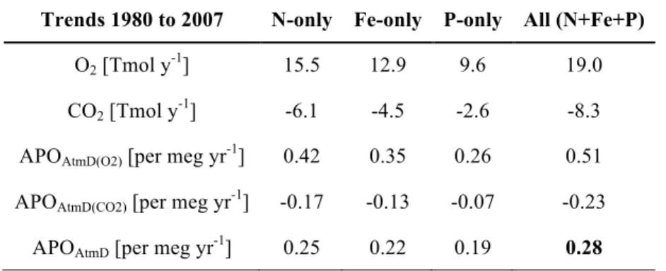
Table S5. Trends in air–sea flux of O₂, CO₂ and APO due to anthropogenic aerosol deposition

Trends 1980 to 2007 N-only Fe-only P-only All (N+Fe+P)

O₂ [Tmol y^-1] 15.5 12.9 9.6 19.0 CO2 [Tmol y^-1] -6.1 -4.5 -2.6 -8.3

APOAtmD(O2) [per meg yr^-1] 0.42 0.35 0.26 0.51

APO_AtmD(CO2) [per meg yr^-1] -0.17 -0.13 -0.07 -0.23 APOAtmD [per meg yr^-1] 0.25 0.22 0.19 0.28

Table S6. Contributions to the uncertainty in ΔAPOClimate (1σ)

Source of uncertainty Uncertainty in ΔAPOClimate trend (in per meg yr^-1) Measurement uncertainties

Corrosion 0.30

Leakage 0.20

Desorption 0.10

Scale Error 0.39

Thermal Fractionation 0.06

Other uncertainties

ΔAPOFF 0.32

ΔAPOCant 0.14

ΔAPOAtmDep 0.14

Land oxidative ratio αB 0.14

Quadrature sum 0.68

Generated by isolating contributions to the 10⁶-member ensemble, except the land oxidative ratio, which was estimated by differentiation of the central case where αB =1.05 (see Methods).