Spline-based model speciﬁcation and prediction for least squares and quantile regression

(1)

Spline-based model specification and prediction for least squares and

quantile regression

Dissertation zur Erlangung des Grades eines Doktors der Wirtschaftswissenschaft

eingereicht an der Wirtschaftswissenschaftlichen Fakult¨ at der Universit¨ at Regensburg

vorgelegt von: Kathrin Kagerer

Berichterstatter:

Prof. Dr. Rolf Tschernig, Universit¨ at Regensburg Prof. Dr. Harry Haupt, Universit¨ at Bielefeld

Tag der Disputation: 16. M¨ arz 2012

(2)

(3)

List of Figures

1.1 Different bases and examples for linear combinations of the basis functions. . . 5 1.2 B-spline bases, sums and linear combinations for different ordersk with

equidistant knots. . . 8 1.3 B-spline bases, sums and linear combinations for different ordersk with

equidistant knots where one knot position is multiple occupied. . . 10 1.4 B-spline basis functions of different orderskwith non-equidistant knots

and their sum. . . 11 1.5 Monotonically weighted B-spline basis functions and their first derivative. 13 1.6 Apart from one time monotonically weighted B-spline basis functions

and their first derivative. . . 13 1.7 Loss functions for least squares estimation and quantile regressions. . . 23 1.8 Results from quantile regressions for simulated data. . . 24 1.9 Scatter plot with estimated quadratic quantile regression curves and

estimated parameters for simulated data. . . 25 1.10 Conditional ϑ-quantiles for heteroskedastic logistic error distribution. . 27 1.11 Scatter plot with crossing estimated quantile regression lines for simu-

lated data. . . 31 5.1 Cubic B-spline basis functions for equidistant knot sequence and one

additional basis function. . . 50 5.2 Plot of knot positions versus estimated spline parameters for the mo-

torcycle data. . . 54 5.3 Function f1(x) and ASEP results from the simulation. . . 59

(6)

5.4 Function f2(x) and ASEP results from the simulation. . . 59

5.5 Function f₃(x) and ASEP results from the simulation. . . 60

5.8 Function f₆(x) and ASEP results from the simulation. . . 61

5.9 Motorcycle data example and ASEP results for predictions to the right. 64 5.10 Motorcycle data example and ASEP results for predictions to the left. 64 5.11 LIDAR example and ASEP results. . . 65

5.12 Average ASEP results for f1(x) and a 1-, . . ., 6-intervals horizon. . . . 67

5.14 Average ASEP results for f₃(x) and a 1-, . . ., 6-intervals horizon. . . . 68

5.17 Average ASEP results for f₆(x) and a 1-, . . ., 6-intervals horizon. . . . 69

(7)

List of Tables

5.1 Classification and summary of prediction methods. . . 55 5.2 Share ofRreplications where the prediction method with lowest ASEP

for knot interval Im is the same as the method with lowest ASEP for the majority of knot intervals It, t = s, . . . ,m−1, and share of R×(_m−_s)cases where the prediction method with lowest ASEPfor knot interval It, t =s+1, . . . ,m, is the same as for knot interval It−1. 62

(8)

(9)

1 Introduction and overview

1.1 Introduction and methodological background

Systema [. . .] maxime probabile valorum incognitarum [. . .] id erit, in quo quadrata differentiarum inter [. . .] valores observatos et computatos sum- mam minimam efficiunt.

[. . .] that will be the most probable system of values of the unknown quantities [. . .] in which the sum of the squares of the differences between the observed and computed values [. . .] is a minimum.

This insight still is of crucial interest more than 200 years after Carl Friedrich Gauss stated it in 1809 (Gauss, 1809, p. 245, translation from Davis, 1857, p. 260). The method of least squares is historically used to describe the course of planets by Gauss (1809) and Legendre (1805) who independently suggested the same method. Today there are many more fields that apply the method of least squares in regression analysis.

Among these are geography, biology/medicine and economics.

Years before Gauss’ and Legendre’s method of least squares, Laplace suggested to minimize the sum of absolute differences between observed and calculated observations (Laplace, 1789). Portnoy & Koenker (1997) provide a historical review and a detailed comparison of both methods. Minimizing the sum of absolute differences, as introduced by Laplace, is a special case of the method which is nowadays known as quantile regression.

(10)

1.1.1 Classical linear least squares regression analysis

Classical linear least squares regression can be applied to quantify the change of the expected outcome of the response y given x1 and potential other factors x2, . . . ,xq

when x₁ varies by some amount while the other covariates x2, . . . ,xq are held fixed.

Accordingly, the expected value of y given the covariates x₁, . . . ,xq, E(y|x₁, . . . ,xq), is a function of the covariates, that is, it can be expressed as

E(y|x₁, . . . ,xq) = f(x₁, . . . ,xq), (1.1)

where f is a (unknown) function that describes the relationship between E(y|x₁, . . . ,xq) and the covariates x1, . . . ,xq. Hence, the relationship between y and f(x1, . . . ,xq) is given by

y = f(x1, . . . ,xq) +u, (1.2)

where E(u|x₁, . . . ,xq) =0.

An often applied choice when estimating the function f, is to assume a linear relationship between E(y|x1, . . . ,xq)and the covariatesx1, . . . ,xq. That is, the functional form f is a linear combination of the covariates,

f(x₁, . . . ,xq) = _β₀+_β₁x₁+. . .+_β_qxq, (1.3)

where β0, . . . ,βq are unknown parameters that need to be estimated. For a given sample i =1, . . . ,n the parameters may be estimated by solving

˜ min

β₀,..., ˜βq∈_R

∑

n i=₁

yi−(β^˜0+β^˜1x1+. . .+β^˜qxq)².

Hence, the estimates for the parameters β0, . . . ,βq are those that minimize the sum of squared differences between the observed values y_i and the computed values yˆ_i = βˆ0+_β^ˆ₁x_i1+_{. . .}+_β^ˆ_qx_iq. That is, the parameters are estimated by applying Gauss’

method of least squares.

To allow for other functional forms, E(y|x₁, . . . ,xq)could, for example, be expressed as linear combination of higher order polynomials or other transformations of the covariates. This implies a possibly extensive specification search for f. To avoid this,

(11)

non- or semiparametric specifications for f can be applied. Spline regression is one of these nonparametric methods. An outline of splines and spline regression is given in Section 1.1.2.

For simplification, consider a bivariate relationship between one covariate x and the response y. Then, Equation (1.1) simplifies to

E(y|x) = f(x). (1.4)

If f is incorrectly specified for the estimation, several conclusions (e.g. interpretations of marginal effects and hypothesis tests) that build on a correctly specified model are invalid. Hence, a correct specification of f is crucial.

1.1.2 Splines

Basis functions

Truncated power basis and splines Piecewise polynomial functions constitute an easy approach to adopt a flexible functional form without being demanding to im- plement. These functions can be generated in different ways. An intuitive way to understand the main principle is to consider the truncated power basis (see for example Ruppert et al., 2003, ch. 3, Dierckx, 1993, ch. 1.1, de Boor, 2001, ch. VIII as general references). Consider a straight line on some interval [κ0,κm+1] (e.g.

[κ₀,κ_m+1] = [min_i(x_i), max_i(x_i)] for a sample i = 1, . . . ,n) with a kink at some position κ1 where κ0 < _κ₁ < _κ_m₊₁. It can be described by a weighted sum (i.e. a linear combination) of the basis functions 1, x and (x−κ1)+, where the truncation function

(x−_κ₁)+ =







x−κ1 for x ≥κ1

0 else

gives the positive part of x−κ1. The reasoning for the basis functions 1, x and (x−κ₁)+ is as follows: To obtain a straight line f that is folded atκ₁ but continuous there, this function f can be written as β0+_β₁x forx <_κ₁and as β⁰₀+ (_β₁+_α₁)x for x ≥ κ1. That means, the slope is β1 until x = κ1 and from x = κ1 on the

(12)

slope is changed by α₁. As f is constrained to be continuous at κ₁, this requires β0+_β₁_κ₁ = _β⁰₀+ (_β₁+_α₁)_κ₁ to hold or equivalently β⁰₀ = _β₀−_α₁_κ₁. Overall, f then is given by

f(x) = (β0+β1x)·I_{_x<_κ₁}+ β⁰₀+ (β1+α1)x

·I_{_x_≥_κ₁_}

= (β0+β1x)·I{x<_κ₁}+ (β0+β1x+α1(x−κ1))·I{x≥_κ₁}

=β0+β1x+α1(x−_κ₁)I{x≥κ₁}

=_β₀+_β₁x+_α₁(x−_κ₁)+

where I{A} is the indicator function which is 1 if A holds and 0 else. That is, f can be written as a linear combination of the basis functions 1, x and (x−κ1)+.

Note that linear least squares regression with a constant and one covariatexhas the two basis functions 1 and x and that for example an additional quadratic term leads to the additional basis function x².

Analogously to the line folded only at κ₁, a line folded m times at the positions κ1, . . . ,κm can be written as the weighted sum of the basis functions 1, x, (x− κ1)+, . . . ,(x−κm)+, where the κj’s are called knots. With a proper choice of the knotsκ_j, the functions generated from this basis can approximate other functions rather well. However, it yields a curve with sharp kinks that is not differentiable at the knots.

These sharp kinks as well as the lacking differentiability are often undesirable. Smoother curves can be obtained by using higher powers of the basis functions. The respective basis of degree p≥₀consists of the functions1,x, . . . ,x^p,(x−_κ₁)₊^p_{, . . . ,}(x−_κ_m)₊^p, where (x−κj)^p₊ := (x−κj)+p

and 0⁰ := 0, and is called truncated power basis of degree p. The truncated power function (x−κ_j)₊^p is (p−1)-times continuously differentiable atκj. Hence, also the linear combinations (called splines, Ruppert et al., 2003, p. 62) of the truncated power basis functions are (p−1)-times continuously differentiable at the knots κ_j, j =1, . . . ,m.

Additionally including lower powers (< p) of (x−_κ_j)+ in the basis, changes the differentiability properties. That is, if the basis consists for example of the functions 1,x, . . . ,x^p,(x−κ₁)₊^p, . . . ,(x−κ₁)₊^p⁻^m¹⁺¹,(x−κ2)₊^p, . . . ,(x−κm)^p₊, the resulting linear combinations are (p−m₁)-times continuously differentiable atκ1 and (p−₁)- times continuously differentiable atκ2, . . . ,κm, where m1can be regarded as multiplic-

(13)

ity of the knotκ₁(e.g. Eubank, 1984, p. 447f.). Form_j = p+1, functions constructed as linear combination from the truncated power basis functions of degree phave a dis- continuity/jump atκj. Ifmj >1, the respective knots and basis functions are denoted as(x−κ_j)₊^p, . . . ,(x−κ_j+m_j−1)^p₊⁻^m¹⁺¹, whereκ_j =. . .=κ_j−m_j+1. That is, the knot κj has multiplicity m_j (and so have κj+1, . . . ,κj−m_j+1 where m_j = _{. . .} = m_j−m_j+1).

This notation is consistent with the notation for the equivalent B-spline basis which is described later on. Further, the truncated power basis of degree pthus always consists of p+₁+m basis functions that are identified once the knot sequence is given.

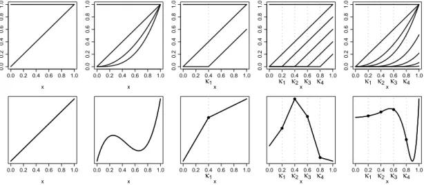
The panels in the upper row of Figure 1.1 show the functions of the above described bases: the basis for linear functions (1, x), the basis for cubic functions (1,x, x², x³), the truncated power basis of degree 1 with one knot at 0.4 (1, x, (x−_0.4)+), the truncated power basis of degree 1 with four knots at0.2, . . ., 0.8 (1, x, (x−0.2)+, . . ., (x−0.8)+) and the truncated power basis of degree 3 with four knots at 0.2, . . .,0.8 (1, x, x², x³, (x−_0.2)³₊,. . .,(x−_0.8)³₊). Additionally, the lower row shows an arbitrary example for a linear combination of the basis functions for each of the illustrated bases.

0.0 0.2 0.4 0.6 0.8 1.0

0.00.20.40.60.81.0

x

0.0 0.2 0.4 0.6 0.8 1.0 x

0.0 0.2 0.4 0.6 0.8 1.0

0.00.20.40.60.81.0

x

0.0 0.2 0.4 0.6 0.8 1.0 x

0.0 0.2 0.4 0.6 0.8 1.0

0.00.20.40.60.81.0

x

κ1

0.0 0.2 0.4 0.6 0.8 1.0

κ1x

●

0.0 0.2 0.4 0.6 0.8 1.0

0.00.20.40.60.81.0

x

κ1 κ2 κ3 κ4

0.0 0.2 0.4 0.6 0.8 1.0

κ1 κ2xκ3 κ4

●

0.0 0.2 0.4 0.6 0.8 1.0

0.00.20.40.60.81.0

x

κ1 κ2 κ3 κ4

0.0 0.2 0.4 0.6 0.8 1.0

κ1 κ2xκ3 κ4

● ● ●

●

Figure 1.1: Top: different bases (from the left): basis functions for straight line, for cubic polynomial, for straight line with one kink, for straight line with four kinks, for cubic polynomial with four kinks. Bottom: arbitrary examples for linear combinations of the basis functions from the corresponding upper panel.

A disadvantage of the truncated power basis is that the basis functions are correlated and hence estimation results are often numerically instable (Ruppert et al., 2003, p. 70).

(14)

An equivalent basis that does not have this problem (Dierckx, 1993, p. 5, Ruppert et al., 2003, p. 70, de Boor, 2001, p. 85f.) and leads (apart from computational accuracy) to the same fit on [κ0,κm+1] (Ruppert et al., 2003, p. 70) is the B-spline basis of order k = p+1 ≥1 where p is the degree of the truncated power basis. In the following, B-splines are introduced.

B-spline basis and splines In a nutshell, the functions from the B-spline basis are piecewise polynomial functions of order k that are connected at the knots and have only small support. Then the spline of order k, which is a linear combination of the basis functions, is also a piecewise polynomial function of orderk. It exhibits the same properties as the respective linear combination of the functions from the truncated power basis of degree p = k−1 with the same knots κ1, . . . ,κm. A short review concerning B-splines can be found e.g. in the work of Eilers & Marx (1996) who summarize the definition and properties of B-splines while de Boor (2001), Dierckx (1993) and Ruppert et al. (2003) provide a more extensive discussion of splines.

To derive the B-spline basis of order k, some definitions are necessary. Let κ = (κ₋₍_k₋₁), . . . ,κ_m+k) be a non-decreasing sequence of knots (i.e. κ₋₍_k₋₁) ≤ . . . ≤ κm+k), where at most k adjacent knots coincide (i.e. κj 6= _κ_j₊_k). The two bound- ary knots κ0 and κm+1 define the interval of interest and the m knots κ1, . . . ,κm

are called inner knots. The remaining 2(k−1) exterior knots κ₋₍_k₋₁₎, . . . ,κ−1 and κm+2, . . . ,κm+kare required to ensure regular behavior on the interval[_κ₀,κm+1]. The B-spline basis functions (also called B-splines) are denoted asB^κ,k_j ,j =−(k−1), . . . ,m.

B-splines can be motivated in different ways. One of them is to derive them by using divided differences (for a definition of divided differences and the corresponding representation of B-splines see for example de Boor, 2001, p. 3, 87). Another way that does not involve the definition of divided differences and can be shown to lead to the same result (cf. de Boor, 2001, p. 88) is to recursively calculate the B-splines of order k > 1 from the B-splines of lower order using the recurrence relation from de Boor (2001, p. 90)

B^κ,k_j (x) = ^x−κ_j κj+k−1−_κ_j^B

κ,k−1

j (x) − ^x−κ_j+k

κj+k−_κ_j₊₁^B

κ,k−1 j+1 (x),

(15)

where

B^κ,1_j (x) = (_κ_j₊₁−x)⁰₊−(_κ_j−x)⁰₊ =







1 for κ_j ≤x <κ_j+1

0 else

is the B-spline of order1(de Boor, 2001, p. 89) and the indexj runs from−(k−1) to m. To obtain the properties of B-splines on the complete interval [κ0,κm+₁] but not only on[_κ₀,κm+1), the definition ofB_m^κ,1 and B^κ,1_m₊₁is modified such that B^κ,1_m (x) = 1 for x=κm+1 and B_m^κ,1₊₁(x) = 0 for x=κm+1 (cf. de Boor, 2001, p. 94).

For equidistant knots, that is ∆κj =κ_j−κ_j−1=: h for j=−(k−1) +1, . . . ,m+ k, it can be shown (based on an extension of Problem 2 from de Boor, 2001, p. 106) that the function B^κ,k_j can also be written as

B^κ,k_j (x) = ¹

h^k⁻¹(k−₁)_! ^∆

k(_κ_j₊_k−x)^k₊⁻¹

where∆^k :=∆(∆^k⁻¹).

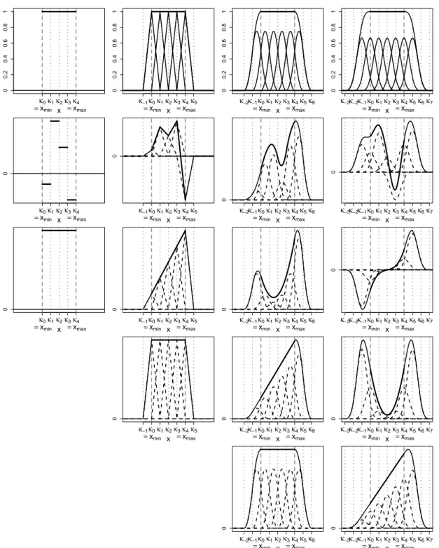
Figure 1.2 gives examples for B-spline bases of different orders k for an equidistant knot sequence κ with m = 3 inner knots. In the first row, the basis functions B^κ,k_j , j=−(_k−₁), . . . ,m, and their sum are shown. Further details of Figure 1.2 are given in the following when the respective features are explained.

B-splines have several useful properties. Firstly, they form a partition of unity on the interval [κ0,κm+1], that is, on [κ0,κm+1] it holds that

∑

m j=−(k−1)

B^κ,k_j (x) = 1 (1.5)

(de Boor, 2001, p. 96). This can be observed in the first row of Figure 1.2. Moreover, each of the basis functions has only small support. More precisely, the support of the function B^κ,k_j is the interval(κ_j,κ_j+k) (de Boor, 2001, p. 91), henceB^κ,k_j (x)·B^κ,k_j₊_d(x) is zero for|d| ≥ k, which is the reason for the numerical stability mentioned on page 6.

Further, the B-splines are up to (k−mj−1)-times continuously differentiable at the knot κ_j and the (k−m_j)th derivative has a jump at κ_j where m_j is the multiplicity of the knot κj (e.g. κj = _{. . . ,}_κ_j₊_m_j₋₁) (Dierckx, 1993, p. 9, de Boor, 2001, p. 99).

This property carries over to linear combinations of the basis functions (called spline,

(16)

x κ0κ1κ2κ3κ4

=xmin =xmax

00.20.40.60.81

x κ−1κ0κ1κ2κ3κ4κ5

=xmin =xmax

00.20.40.60.81

x κ−2κ−1κ0κ1κ2κ3κ4κ5κ6

=xmin =xmax

00.20.40.60.81

x

κ−3κ−2κ−1κ0κ1κ2κ3κ4κ5κ6κ7

=xmin =xmax

00.20.40.60.81

x κ0κ1κ2κ3κ4

=x_min =x_max

0

=x_min =x_max

0

=x_min =x_max

0

x

=x_min =x_max

0

x κ0κ1κ2κ3κ4

=xmin =xmax

0

=xmin =xmax

0

=xmin =xmax

0

x

=xmin =xmax

0

=xmin =xmax

0

=xmin =xmax

0

x

=xmin =xmax

0

=xmin =x_max

0

x

=xmin =x_max

0

Figure 1.2: B-spline bases, sums and linear combinations for different ordersk with equidistant knots andm=3. First row: B-spline basis functions of orders 1, 2, 3 and 4, and their sum, which is 1 on [κ₀,κ_m+1]. Second row: arbitrarily weighted B-spline basis functions of orders 1, 2, 3 and 4, and their sum. Third row: B-spline basis functions of order 1, 2, 3 and 4, weighted such that their sum is a polynomial of degreek−1on[κ₀,κ_m+1]. Fourth row:

B-spline basis functions of orders 2, 3 and 4, weighted such that their sum is a polynomial of degree k−2 on [κ₀,κ_m+1]. Fifth row: B-spline basis functions of orders 2, 3 and 4, weighted such that their sum is a polynomial of degree k−3 on[κ₀,κ_m+1].

(17)

de Boor, 2001, p. 93), that is, the functions B_α^κ,k(x) =

∑

m j=−(k−1)

αjB^κ,k_j (x)_, (1.6)

where α = _α₋₍_k₋₁₎ _{. . .} _α_m⁰, are also (k−mj−1)-times continuously differentiable at the knot κ_j. The second row of Figure 1.2 shows examples for linear combinations of the basis functions from the first row with arbitrarily chosen αj.

The linear combinations of the B-spline basis functions of order k can generate all polynomial functions (in contrast to piecewise polynomial functions) of degree smaller than k on the interval [_κ₀_,_κ_m₊₁]. Note that this is also a spline/polynomial of order k. This justifies the use of the notation order instead of degree since all polynomials of degree<kare polynomials of order k. In the third (fourth, fifth) row of Figure 1.2, examples for polynomials of degree k−₁ (k−₂, k−₃) are given for k ≥ ₁ (k ≥ ₂, k ≥3).

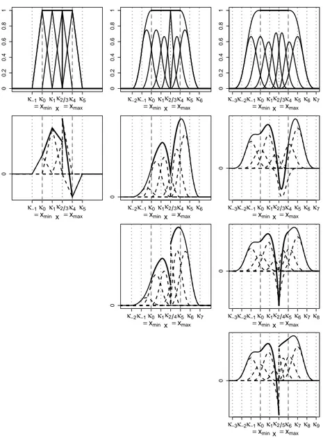
The first two rows of Figure 1.3 show B-spline bases withk=2, 3, 4where two knots of the knot sequenceκcoincide. In the first row,αj =₁for all j,j =−(k−₁)_{, . . . ,}m, and in the second row, theαj are chosen arbitrarily. Fork =2 the resulting spline now has a jump where the double knot is placed. For k = 3 the spline is still continuous, but its derivative is not, and for k =₄ the first derivative is also continuous, but the second derivative is not. For k = 1 no graphic is presented since twofold knots with κ_j =κ_j+1 do not make sense in this case, because B^κ,1_j would be zero and could be excluded from the basis. The third row of Figure 1.3 shows weighted B-spline bases and the respective resulting splines for k = 3 and k = 4 where κj = κj+₁ = κj+₂

for some j (i.e. m_j = 3). Then the spline of order 3 has a jump at κ_j and the spline of order 4 is continuous. For k = ₂ one of the threefold knots is meaningless (as discussed for k=1and twofold knots). In the last line of Figure 1.3, a spline of order 4 is shown that has a jump at a fourfold knot position (m_j =4 there).

To contrast equidistant knot sequences to those with non-equidistant knots, Figure 1.4 exemplarily shows B^κ,k_j , j = −(k−1), . . . ,m, and ∑^m_j=−(k−1)B^κ,k_j (x) for a non- equidistant knot sequence. This is analogous to the first row of Figure 1.2 with the only difference that the knots are not equidistant and hence the basis functions B^κ,k_j look different. But still they sum up to unity on [κ0,κm+1].

(18)

x κ−1κ0κ1κ2 3κ4κ5

=xmin =x_max

00.20.40.60.81

x

κ−2κ−1κ0κ1κ2 3κ4κ5κ6

=xmin =x_max

00.20.40.60.81

x

κ−3κ−2κ−1κ0κ1κ2 3κ4κ5κ6κ7

=xmin =x_max

00.20.40.60.81

x κ−1κ0κ1κ2 3κ4κ5

=xmin =xmax

0

x

=xmin =xmax

0

x

=xmin =xmax

0

x

=xmin =xmax

0

x

=xmin =xmax

0

x

=x_min =x_max

0

Figure 1.3: B-spline bases, sums and linear combinations for different ordersk with equidistant knots where one knot position is multiple occupied. First row: B-spline basis functions of orders 2,3 and 4, where κ₂ =κ₃, and their sum which is 1 on [κ₀,κ_m+1]. Second row:

arbitrarily weighted B-spline basis functions of orders 2,3 and 4, where κ₂ = κ₃, and their sum. Third row: arbitrarily weighted B-spline basis functions of orders 3 and 4, where κ₂ = κ₃ =κ₄, and their sum. Fourth row: arbitrarily weighted B-spline basis functions of order4, where κ₂=κ₃ =κ₄ =κ₅, and their sum.

Derivative and monotonicity The first derivative of the B-spline functions is

∂B^κ,k_j (x)

∂x = ^k−1 κj+k−1−_κ_j^B

κ,k−1

j (x)− ^k−1

κj+k−_κ_j₊₁^B

κ,k−1

j+1 (x) (1.7)

(19)

x κ0 κ1κ2κ3κ4

=xmin =xmax

00.20.40.60.81

x κ−1κ0 κ1κ2κ3κ4κ5

=xmin =xmax

00.20.40.60.81

x

κ−2κ−1κ0 κ1κ2κ3κ4κ5κ6

=xmin =xmax

00.20.40.60.81

x

κ−3κ−2κ−1κ0 κ1κ2κ3κ4κ5κ6κ7

=xmin =xmax

00.20.40.60.81

Figure 1.4: B-spline basis functions of orders 1, 2, 3 and 4 with non-equidistant knots (m=3), and their sum which is 1 on[κ₀,κ_m+1].

for k > ₁ (de Boor, 2001, p. 115). For k = ₁ it is defined to be 0 according to the argumentation in de Boor (2001, p. 117). Hence, the first derivative of a B-spline of order k is a spline of order k−1 since it is a linear combination of B-splines of order k−₁. From Equation (1.7) it can be shown that the first derivative of a spline as linear combination of the B-spline basis functions is given by

∂B^κ,k_α (x)

∂x = ^∂

∂x

∑

m j=−(k−1)

α_jB^κ,k_j (x) = (k−1)

m+1 j=−(

∑

k−1)

α_j−α_j−1

κj+k−1−_κ_j^B

κ,k−1

j (x) (1.8) where α₋₍_k₋₁₎₋₁ := 0 =: α_m+1 (de Boor, 2001, p. 116). On the interval [κ0,κ_m+1] it holds that B^κ,k₋₍_k⁻₋¹₁₎(x) = B_m^κ,k₊⁻₁¹(x) =₀ and hence the summation reduces to

∂B^κ,k_α (x)

∂x = (k−₁)

∑

m j=−(k−1)+1

αj−_α_j₋₁ κ_j+k−1−κj

B^κ,k_j ⁻¹(x) (1.9) on[_κ₀_,_κ_m₊₁]. For equidistant knot sequences, Equations (1.7) and (1.8)/(1.9) simplify to

∂B^κ,k_j (x)

∂x = ¹

hB^κ,k_j ⁻¹(x)−¹

hB^κ,k_j₊₁⁻¹(x) and

∂B^κ,k_α (x)

∂x = ¹ h

m+1 j=−(

∑

k−1)

(_α_j−_α_j₋₁)B^κ,k_j ⁻¹(x) = ¹ h

∑

m j=−(k−1)+1

(_α_j−_α_j₋₁)B^κ,k_j ⁻¹(x),

(1.10) respectively, on[_κ₀_,_κ_m₊₁]. Higher order derivatives can also be calculated from Equa- tions (1.7) or (1.8).

(20)

Since all of the terms k−1, κ_j+k−1−κ_j and B^κ,k_j ⁻¹(x), j=−(k−1) +1, . . . ,m are greater or equal to zero (de Boor, 2001, p. 91), the sign of ^∂B^α^κ,k_∂x⁽^x⁾ only depends on the differences α_j−α_j−1 =: δ_j, j = −(k−1) +1, . . . ,m. It can be seen from Equation (1.8) that

α_j≥α_j−1 (i.e.δ_j ≥0), j =−(k−1) +1, . . . ,m, (1.11) ensures a completely non-negative first derivative of B^κ,kα , and hence Bα^κ,k is monotonically increasing. Analogously, B^κ,kα is monotonically decreasing if

αj≤_α_j₋₁ (i.e.δj ≤₀), j =−(k−₁) +_{1, . . . ,}m. (1.12) If α_j ≥ α_j−1, j = −(k−1) +1, . . . ,m, holds (where α_j 6= 0 for at least one j), it follows that α−(k−1) 6≥ _α₋₍_k₋₁₎₋₁ or αm+1 6≥ _α_m since the auxiliary parameters α₋₍_k₋₁₎₋₁ and αm+1 from Equation (1.8) are zero. This implies that the spline is only monotonically increasing on the interval [κ0,κ_m+1]. Hence, the derivative (1.9) where the sum is indexed from j = −(k−₁) +₁ to j = m and not (1.8) with j = −(k+1), . . . ,m+1 has to be regarded. For αj ≤ αj−1 these considerations apply analogously.

Equations (1.11) and (1.12) can also be written in matrix notation as Cα≥0 with C =





−1 1

... ...



 and C=





1−1 1−1

1−1

... ...



,

respectively.

Trivially, fork =1the conditions (1.11) and (1.12) are each necessary and sufficient conditions for monotonicity. For k > 1 this issue is illustrated in Figures 1.5 and 1.6 for equidistant knot sequences but the same reasoning holds for non-equidistant knot sequences. The upper rows of both figures show splines B^κ,kα and the underlying basis functions B^κ,k_j weighted by α_j while the lower rows picture the respective derivatives

1

h∑^m_j₌₋₍⁺¹_k₋₁₎(_α_j−_α_j₋₁)B^κ,k_j ⁻¹(x) = ¹_h_∑^m_j₌₋₍⁺¹_k₋₁₎_δ_jB^κ,k_j ⁻¹(x)and the underlying basis functions B^κ,k_j ⁻¹weighted by δj. Figure 1.5 gives an example whereαj≥αj−1 (i.e.

δ_j ≥0) holds for all j=−(k−1) +1, . . . ,m. Hence all splines in the upper row are monotonically increasing on the interval[_κ₀_,_κ_m₊₁]. In contrast, in Figure 1.6 the con- dition δj ≥0 is hurt for some j. For k =2 and k =3this implies a derivative that is

(21)

negative within a certain interval and hence the spline is non-monotone on[κ0,κ_m+₁]. But for k=₄ (and also for k≥₅ what is not illustrated here) some combinations of αj exist where the respective splineB^κ,kα is monotonically increasing on[κ0,κm+1]even if δ_j is negative for some j. That is, for k ≤ 3 the conditions (1.11) and (1.12) are each necessary and sufficient for monotonicity and for k ≥ ₄ they are each sufficient but not necessary for monotonicity. A compendious discussion can also be found in Dierckx (1993, sec. 7.1).

=xmin =xmax

0

x

κ−2κ−1κ0κ1κ2κ3κ4κ5κ6

=xmin =xmax

0

x

=xmin =xmax

0

x κ0κ1κ2κ3κ4

=xmin =xmax

0

κ−1 κ5

=xmin =xmax

0

κ−2 κ6

x

=xmin =xmax

0

κ−3 κ7

Figure 1.5: Top: monotonically weighted B-spline basis functions of orders2,3and4, and their sum. Bottom: first derivative of the spline from the top with underlying respectively weighted B-spline basis functions.

=xmin =xmax

0

x

=xmin =xmax

0

x

=xmin =xmax

0

x κ0κ1κ2κ3κ4

=xmin =xmax

0

κ−1 κ5

=xmin =xmax

0

κ−2 κ6

x

=xmin =xmax

0

κ−3 κ7

Figure 1.6: Top: apart from one time monotonically weighted B-spline basis functions of orders 2,3 and 4, and their sum. Bottom: first derivative of the spline from the top with underlying respectively weighted B-spline basis functions.