A psychological approach to individual differences in intertemporal consumption patterns1
Hermann Brandstätter Werner Güth
Johannes-Kepler-University Humboldt-University
Linz, Austria Berlin, Germany
1 A preliminary version of the paper was presented at the IAREP workshop on Individual Differences in Economic Behaviour and Games. International Center for Economic Research (ICER), Torino, March 13-14, 1998. We thank Ekkehart Böhmer for stylistic advice.
Abstract
When people decide about saving and consumption across the various periods of their life time they take into account their life expectancy when comparing present and future needs and resources for satisfying them. The experimental design, applied at two sites (Humboldt-University at Berlin and Johannes-Kepler-University, Linz), aims at simulating a sequence of at least three, at most six saving vs. consumption decisions, depending on a stochastic manipulation of changes in life expectancy. In this report we focus on how personality characteristics influence the amount of consumption in single periods of life depending on life expectancy changes which may render previous consumption rates as too low or too high. According to Gray (1987) it was predicted and found that unstable introverts respond most, and stable extroverts least to this kind of ‘punishment’. In addition, some exploratory findings involving the personality dimensions conscientiousness and tough-mindedness are reported.
Key words
Experimental economics; personality; intertemporal consumption and saving; individual differences.
Introduction
Saving behavior is crucial for economic development (see for a survey Anderhub et al., 1996). Macroeconomically, saving reduces consumption and thereby employment, but it may also inspire investment demand via an increased capital supply what in the short and long run offsets its direct detrimental effect on employment. In microeconomics, deterministic and stochastic life cycle models (see Hall, 1978, for a survey) have been constructed which assume that people rely on intertemporal utility functions in choosing their consumption pattern over lifetime. Psychologically, saving or, more generally, intertemporal decision tasks, can be viewed as intrapersonal decision conflicts (see, for instance, Frank, 1996). A saving pattern is an attempt to balance present and future needs, i. e., a way to resolve the conflict between one’s present and future ego.
As often it is difficult, if not impossible, to test such models by field data. What seems to be possible at most is to validate or reject certain requirements for intertemporal utilities like their consistency over time. This quite naturally leads to attempts to analyze saving behavior experimentally. Here we do not want to look at all the evidence, but focus on a particular study which also asked the participants to answer the 16-PA personality questionnaire (Brandstätter, 1988) allowing to test some hypotheses about saving behavior derived from personality theory. When answering this personality questionnaire participants must locate themselves on 16 dimensions, each represented by 2 bipolar scales to achieve a higher reliability of the measures and to allow internal consistency checks. We propagate its general use since it provides some control of what kind of people participate in the study and since it allows, as demonstrated here, to account in a systematic way for individual differences in behavior.
Method
The saving game
In the computerized experiment participants (students) had to play 12 rounds of a
‘saving game’ (Anderhub et al., 1996). In each game one is given an initial endowment of 11.92 experimental currency units (‘ECU’) which one can spend in the course of the saving game. Participants knew that a ‘life’ lasts for at least 3 and for at most 6 periods.
How long it lasts depends on chance moves. Before the game starts, the participants are informed that the probability of reaching the periods 4, 5, and 6 depends on chance in the following way: There are three dices, a red, a yellow, and green one. The meaning of the colors will be explained later. After having decided about the amount C1 of money to be spent in the first period, one of the three dices is eliminated with a probability of 1/3.
After the second move (deciding about consumption C2 in period 2) one of the remaining two dices is eliminated with a probability of ½. Therefore, a red, a yellow, or a green dice is left for determining the survival beyond period 3, 4, and 5. If the green dice is left, the good one, life ends after period 3 only when the number 1 (out of 6) comes up, this means a survival probability of 5/6. The yellow dice ends life with the numbers 1 or 2 (survival probability of 4/6). The ugly red dice brings life to an end with the numbers 1, 2, and 3 (survival probability of 3/6). The remaining dice is applied for moving (or not moving) from period 3 to period 4, from period 4 to period 5, and from period 5 to period 6.
Assuming that the participants understand the instruction, they know right from the beginning that the probabilities of survival after period 3 change from an initial proba- bility of 2/3 [(5/6+4/6+3/6)/3 =8/12] depending on random selection of the dices. If the green dice is eliminated first, the survival probability decreases to 7/12 [(4/6+3/6)/2]. If
the red dice is eliminated first, the survival probability increases to 9/12 [(5/6+4/6)/2].
The initial elimination of the yellow dice does not change the survival probability [(5/6+3/6)/2=8/12]. The survival probabilities change again when one of the remaining two dices is eliminated. Depending on the dice finally left, the survival probabilities are 6/12 (red), 8/12 (yellow), and 10/12 (green).
Although the (updated) termination probabilities (the instructions did not speak of probabilities, but only of termination numbers of the dices) are easily derived, it is practically impossible to compute the saving pattern maximizing the intertemporal utility function.
Permutations of the elimination sequence (green - yellow - red)
There are six permutations of the green - yellow - red sequence of dice elimination.
The order of permutations is randomly varied for each participant, and each participant plays the six permutations twice (two cycles of games, each cycle in a different random order of permutations).
Permutations
1 2 3 4 5 6
green yellow green red yellow red
yellow green red green red yellow
red red yellow yellow green green
Intertemporal utility function2
The participant ‘earns’ ECU-units equivalent to the product of the consumption Ct in the single periods t (up to six periods).
UΠ = C1 x C2 x...x CT
Here, T is the stochastically determined length of life with T =3, 4, 5, or 6. In case of T<6 all money, kept for the time after period T, is lost. On the other hand, leaving too little or even nothing for the last period T results in a low payoff UΠ , or even UΠ = 0.
Since a participant experiences 12 successive ‘lives’, one has to specify how the 12 payoffs UΠ in runs 1 to 12 of the saving game determine his/her monetary win. Instead of imposing that the monetary win is either the average of 12 payoffs UΠ or a randomly selected value UΠ, participants were asked to choose for themselves which payment they prefer.
Subjects
The experiments were run mostly with students of economics or business administration at two sites, at the Humboldt University (Berlin) with 50 participants, and at the Johannes-Kepler-University (Linz) with 117 subjects3. There were minor
2 In Berlin, there was another condition, where the participant ‘earned’ the square root of each consumption added up for all survival periods: UΣ = C1 + C2 +...+ CT . This condition, where the intertemporal utility is rather flat, i. e., the same absolute or relative deviations cause less strong effects, will not be considered in the present report.
3 The authors thank Vital Anderhub, Wieland Müller, and Martin Strobel (Humboldt University) and Willy Kriz (Johannes-Kepler-University) for their contributions in planning, running, and analyzing the
differences between the Berlin and Linz procedure which can be neglected in the present context.
Personality scales
Before playing the 12 rounds of the saving game participants are asked to fill out the 16PA-personality adjective scale designed by Brandstätter (1988) as a short measure of Cattell’s five global personality dimensions conscientiousness (self-control), emotional stability (the opposite of neuroticism), independence, tough-mindedness, and extroversion (cf. Schneewind, Schröder & Cattell, 1983).
Participants’ perceptions of the experimental situation
The effects of personality characteristics on game behavior are supposed to be mediated by the way people perceive the experimental situation. Therefore, after finishing the game, the participants were asked to indicate on adjective rating scales (Brandstätter, 1990) how they had experienced the game situation.
Hypotheses
How can we explain the widely varying intertemporal consumption patterns by taking into account the interplay between the structure of the situation as given by the experimental design, and the structure of the personality assessed by the 16PA?
If someone has spent much in the first and second period and realizes that finally the green dice will be applied for determining the survival beyond period 3, s/he is supposed to feel punished by his/her fate, just as someone who has spent little in the early periods
experiment. See Anderhub et al. (1996) for a detailed report on the experiment which did not refer to the
and realizes later that the red dice will determine his/her survival. The reaction towards this kind of punishment should be a change in spending (spending more or spending less) in period 3.
Now we have to ask whether personality theory suggests differential reactions to such punishment. Gray (1987) postulates, referring to research on neuro-physiological processes involved in responses to reward and punishment, that introverts will be more responsive to punishment than extroverts, more so when emotional stability is low.
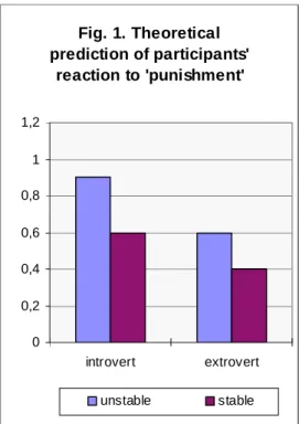
According to Gray (1987, p. 350 f.) no difference is expected between stable introverts and unstable extroverts in sensitivity to punishment. In our context, being more responsive to punishment means showing more pronounced changes in behavior, i. e., in spending more in period 3 if the red dice is applicable, and spending less, if the green dice determines the life expectancy. Gray’s model implies a kind of interaction between emotional stability and extroversion which lets the order of the effects, but not the size of effects unchanged. Figure 1 has been inspired by Figure 14.6 in Gray (1987, p. 351). In the horizontal axis we partition participants into introverts and extroverts, and split the two subgroups into unstable and stable ones. The vertical axis is supposed to measure responsiveness to punishment. How this can be done for the situation at hand will be explained later. Figure 1 shows that emotionally unstable introverts are most, and emotionally stable extroverts least responsive to punishment, and that the difference within the two groups of introverts is larger than that between the two groups of extroverts.
individual differences.
Fig. 1. Theoretical prediction of participants'
reaction to 'punishment'
0 0,2 0,4 0,6 0,8 1 1,2
introvert extrovert
unstable stable
The two basic dimensions - emotional stability and extroversion - can be derived as global (second order) factors from Cattell‘s 16 personality dimensions (according to which the short adjective version 16PA has been designed by Brandstätter, 1988).
Emotionally stable participants describe themselves as emotionally stable and resilient (C)
4, as self confident and carefree (O-). Extrovert persons see themselves as sociable and warm (A), vivacious and sensation seeking (F).
A second hypothesis refers to the subjects‘ choice of the modus of payment, the average payoff across all 12 rounds or the payoff of a single, randomly selected round. It is assumed that conscientious people (people high on norm orientation) prefer the average to the random choice of an outcome as payoff, because they shun higher risks.
Conscientious people describe themselves as conscientious and principled (G), finding reliability and well established traditions important (Q1-), self-controlled and disciplined (Q3). For the situation at hand, norm orientation could also imply accepting the success
4 The letters indicate the labels of the primary factors in Cattell’s 16PF-system.
and failure of all 12 successive ‘lives’. Possibly, participants low in norm orientation opt for the random mode of payment because they can attribute an eventual actual failure to bad luck, thus relying on an ego-defensive attitude what appears as rather typical for low norm orientation.
Results of Hypotheses Testing
There are two sections of results. The first focuses on hypotheses testing, the second reports some additional results of exploratory analyses.
Payoff modus
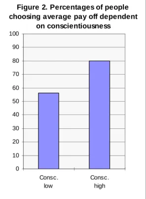
Let us start with the rather simple second hypothesis: Conscientious people prefer the average of all 12 runs, people low in conscientiousness choose the random selection of one run. This is indeed true. Averaged across the two experiments (Berlin and Linz), which show the same pattern of results, 65 % of the participants low in conscientiousness (below median) chose the less risky averaging payoff format, whereas 86 % of high conscientiousness people decided for this format, Chi-Square = 20.07, p = .000 (Figure 2).
Berlin
0 10 20 30 40 50 60 70 80 90 100
Consc.
low
Consc.
high
Figure 2. Percentages of people choosing average pay off dependent
on conscientiousness
Reaction towards ‘punishment’
We expected that anxious subjects (emotionally unstable introverts) are more, stable extroverts less sensitive to punishment. Denote by Cit the average consumption in period t for permutation i. The hypothesis claims a contrast, i. e., a difference of differences in average consumption namely:
x = ((C51+C52+ C61+C62)/4-(C53+C63)/2 - ((C11+C12+ C21+C22)/4-(C13+C23))/2)
x = [(average consumption of the first 2 periods of permutations 5 and 6) minus (average consumption of the third period of permutations 5 and 6)] minus [(average consumption of the first 2 periods of permutations 1 and 2) minus (average consumption of the third period of permutations 1 and 2)]
This difference of differences indicates the strength of the participant’s sensitivity to
‘punishment’ as it is realized with the different elimination sequences of the green, yellow, or red dice. Instead of this kind of difference scores5 we use differences of standardized residuals as dependent variables in testing the effects of personality (emotional stability and extroversion) on sensitivity to punishment. This implies predicting (C53+C63)/2 from (C51+C52+ C61+C62)/4, and predicting (C13+C23))/2 from (C11+C12+ C21+C22)/4, computing the standardized residuals (zresid) and calculating the difference x = zresid[(C53+C63)/2] minus zresid[(C13+C23)/2]. A difference score of zero comes up if a participant chooses under permutation 1 and 2 (the survival probability is that of red dice) as well as under permutation 5 and 6 (the survival probability is that of the green dice) just that consumption in period 3 which would be predicted from the consumption rates of the preceding periods 1 and 2. A difference score of zero or a negative difference score appears, if in period 3 a positive residual under permutation 1 and 2 is neutralized by an equally large or even larger positive residual under permutation 5 and 6, or if a negative residual under permutation 1 and 2 is neutralized by an equally large or larger negative residual under permutation 5 and 6. Therefore, negative difference scores point to inconsistent reactions: adjusting expenditures to the situation given with the red dice, but counteracting the demand of the green dice, or vice versa.
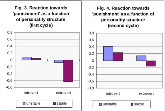
It is claimed that x, represented on the vertical axis of Figures 3, 4, and 5, is larger for introverts than for extroverts, and larger for emotionally unstable than stable participants.
Figure 3 and Figure 4 present the results, separately for the first and second cycle, but combined for both the Berlin and the Linz study, because both studies came up with the same pattern of effects. It shows that stable extroverts are indeed least sensitive to
5 Contrary to differences of residuals, simple differences do not separate ‘real’ differences from regression artefacts (cf. Petermann, F. , 1978).
punishment in both cycles. A 2 (low vs. high stability) by 2 (low vs. high extroversion) by 2 (first vs. second cycle) ANOVA, with cycle as within subject factor, results in a marginally significant main effect of emotional stability, F(1,163) = 2.80, p = 0.096, Eta Squared = 0.017, and a significant main effect of extroversion, F(1,163) = 5.28, p = 0.023, Eta Squared = 0.031. There is no significant interaction between emotional stability and extroversion (p>0.30) although emotional stability makes a larger difference in extroverts than in introverts. The effects are stronger in the second cycle than in the first cycle, F(1,163) = 9.52, p = 0.002. There is no significant interaction of stability or extroversion with cycle (p > .30).
Fig. 3. Reaction towards 'punishment' as a function
of personality structure (first cycle)
-0,8 -0,6 -0,4 -0,2 0 0,2 0,4 0,6 0,8
introvert extrovert unstable stable
Fig. 4. Reaction towards 'punishment' as a function of
personality structure (second cycle)
-0,8 -0,6 -0,4 -0,2 0 0,2 0,4 0,6 0,8
introvert extrovert
unstable stable
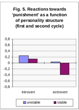
Fig. 5. Reactions towards 'punishment' as a function
of personality structure (first and second cycle)
-0,8 -0,6 -0,4 -0,2 0 0,2 0,4 0,6 0,8
introvert extrovert
unstable stable
Results of exploratory analyses
The results reported in this section do not refer to theoretical predictions but have been selected out of various exploratory analyses if they met the following three criteria:
(a) they are significant (p<0.01, however without alpha-adjustment for post hoc comparisons), (b) they make sense in post hoc interpretations, (c) they are consistent across the two studies (Berlin and Linz) as well as within the studies across the two cycles. We think that they deserve some attention even if their statistical significance is questionable due to the post hoc comparison strategy.
Tough-mindedness
Exploring additional relationships between personality characteristics and adjustments to changes in life expectancy (operationalized as sensitivity to punishment) we found a consistent effect of the dimension tough-mindedness. Tough-minded people (N = 88) describe themselves as tough-minded (I-), realistic and rational (M-). They respond more strongly to unexpected changes in ‘survival’ probabilities than tender-minded people (N
= 79) in both cycles (M = 0.05 vs. M = -0.37, SD = 1,01 vs. SD = 1,47 in the first cycle;
M = 0,35 vs. M = -0.08, SD = 0,98 vs. SD = 1.33 in the second cycle), and the same pattern of results appears in both experiments. Taking an average across both cycles gives a difference with F(1,165) = 6,99, p = 0.009.
Dependence of Payoff on Difference Score
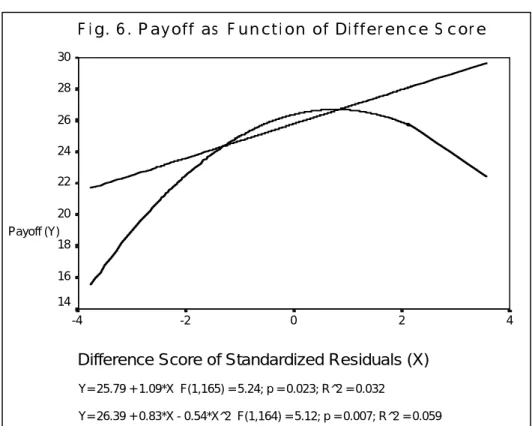
Figure 6 presents payoff as function of the difference score for both cycles combined.
Collapsing the two cycles is justified by the fact that the shape of the curve is basically the same in both cycles. Payoff is highest around a difference score of X = 0.8. Of course, not properly adjusting one’s consumption to changes in survival probabilities diminishes the payoff.
F i g. 6 . P ayoff as F unct i on of Di ffer ence S cor e
Y= 25.79 + 1.09*X F(1,165) = 5.24; p = 0.023; R^2 = 0.032
Y= 26.39 + 0.83*X - 0.54*X^2 F(1,164) = 5.12; p = 0.007; R^2 = 0.059
Difference Score of Standardized Residuals (X)
4 2
0 -2
-4 Payoff (Y)
30 28 26 24 22 20 18 16 14
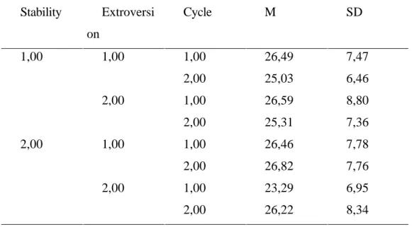
Extroverts, in particular stable extroverts, lack this adjustment because - that was our theoretical prediction - they are less responsive to punishment (Figures 3 and 4). This
explains why stable extroverts get a payoff about one third of a standard deviation less than average in the first cycle (cf. Table 1).
Table 1. Payoff Dependent on Personality and Cycle Stability Extroversi
on
Cycle M SD
1,00 1,00 1,00 26,49 7,47
2,00 25,03 6,46
2,00 1,00 26,59 8,80
2,00 25,31 7,36
2,00 1,00 1,00 26,46 7,78
2,00 26,82 7,76
2,00 1,00 23,29 6,95
2,00 26,22 8,34
Learning from the experience of the first cycle
People generally show a stronger response to unexpected changes in survival probabilities in the second cycle than in the first cycle, F(1,163) = 9.52, p = 0.002, Eta Square = 0.0556 (compare Fig. 3 with Fig. 4). This change is particularly visible in unstable introverts and stable extroverts, although the higher order interaction (cycle by emotional stability by extroversion) is not significant (p>0.10) . As a consequence of those adjustments extroverts, in particular unstable extroverts, improve their payoffs
6 Eta Square is reported as measure of effect size.
from the first to the second cycle whereas introverts do not, possibly because they overreact to punishment in the second cycle. The interaction cycle by stability is significant, F(1,163) = 5.85, p = 0.017, Eta Squared = 0.035. The variance attributed to this interaction derives mainly from the payoff increase of the stable extroverts.
Discussion
In both cycles (remember, a cycle is a run of 6 permutations), emotionally unstable introverts are most sensitive, whereas emotionally stable extroverts are least sensitive to punishment (Figure 3 and Figure 4). This is in line with our predictions derived from the theory of Gray (1987, p. 350 f.) which also states that there is no difference between stable introverts and unstable extroverts in sensitivity to punishment, and that both groups are between (the most sensitive) unstable introverts and (the least sensitive) stable extroverts. According to Gray’s model the polarity introversion-extroversion determines whether a person is more sensitive to punishment or more sensitive to reward, and neuroticism is conceived as a kind of multiplicative factor augmenting the sensitivity to punishment or reward, respectively. This implies a kind of interaction between neuroticism and extroversion which should result in larger differences of punishment effects between unstable and stable introverts than between unstable and stable extroverts. In our data, emotional stability increases the difference in extroverts.
Although the interaction stability by extroversion is not significant, this pattern of results is not in line with the model of Gray.
We may ask why in the saving game the difference in sensitivity to punishment between unstable and stable introverts is not larger than that between unstable and stable extroverts. An answer may be found in the participants’ ratings of how they had perceived the experimental situation. From the 28 adjective rating scales two dimensions
were derived labeled as joyful activation (with marker variables interesting, varied, pleasant) and mastery (easy, clear, comprehensible). Only stable extroverts have high scores on joyful activation, and, on the average, these people are also least sensitive to punishment. Perceiving the game as a stimulating and pleasant experience seems to make less sensitive to punishment.
Still we do not know why the unstable introverts experienced the situation not more negatively than the stable introverts and the unstable extroverts. The answer could be found in the second dimension which we called ‘mastery’: Introverts, whether unstable or stable, have higher scores on mastery than extroverts, i. e., they find the game easier and better comprehensible. Here one may refer to the finding that introverts tend to have better school marks and higher performance scores in cognitive tests (Brandstätter, 1997). If they indeed have a better understanding of the game and of the way how more money can be earned, they will rationally restrain themselves from too strong reactions to ‘punishment’ which would diminish their payoff, thus keeping the difference between unstable and stable introverts in their responses to punishment in the present experiment at a moderate level. Figures 5 shows that, on the average across cycles, payoffs reach their maximum around a difference score of 0.80.
The participants react less to changes of life expectancy, i. e., to ‘punishment, in the first cycle. Obviously, the participants have learned to respond more adequately to stochastic changes in life expectancy. We may also assume that the decisions in the first cycle are somewhat more erratic than in the second cycle. If so, the data of the second cycle are better suited to test Gray’s model, and the results of the second cycle are also in better agreement with the theoretical model.
The sensitivity to reward, in Gray's model lowest in stable introverts and highest in unstable extroverts, is not an issue in our experiment, because reward, i. e., starting with
high consumption and finding out that the red dice will finally be applied (permutations 1 and 2), or starting with low consumption and finding out that the green dice will determine the life expectancy (permutations 5 and 6), does not imply any impetus for change. Without a pressure for change, however, we can not expect any differential effects of personality structure.
That tough-minded (realistic and rational) people adjust their decisions more clearly to changes in survival probabilities makes sense. Their behavior comes close to what economic rationality would prescribe.
Conclusion
Four of the five global personality dimensions (second order factors of Cattell’s system of personality measures) , i. e., conscientiousness, emotional stability, tough- mindedness, and extroversion, proved useful in explaining intertemporal saving vs.
consumption decisions. Although effect sizes as indicated by the percentages of variance explained by the independent variables (Eta Squared) are modest, the consistency of the results across replications (Berlin and Linz) and across cycles within the replications gives them some importance in testing and further developing theoretical ideas in an attempt to explain intertemporal consumption decisions. It seems worthwhile to include short but nevertheless comprehensive and basic measures of personality as well as measures of situation perception in future experiments on economic behavior.
References
Anderhub, V., Güth, W., Härdle, W., Müller, W., & Strobel, M. (1996). On saving, updating and dynamic programming. Unpublished manuscript. Berlin: Humboldt University, Faculty of Economics.
Brandstätter, H. (1988). Sechzehn Persönlichkeits-Adjektivskalen (16 PA) als Forschungsinstrument anstelle des 16 PF [Sixteen Personality Adjective Scales as a research instrument in place of the 16 PF]. Zeitschrift für experimentelle und angewandte Psychologie, 35, 370 - 391.
Brandstätter, H. (1990). Beschreibung von Situationen mit Adjektiv-Skalen (SITAD) [Description of situations on adjective rating scales (SITAD)]. Unpublished manuscript. University of Linz.
Brandstätter, H. (1997). Die Entscheidung für ein Studium als Start der beruflichen Karriere [Starting a career by choosing a course of studies]. In: Rosenstiel, L. v. &
Wins, T. v. Perspektiven der Karriere (p. 85 - 100). Stuttgart: Schäffer-Poeschel.
Frank, B. (1996): The use of internal games: The case of addiction. Journal of Economic Psychology, 17, 651 - 660.
Gray, J. A. (1987). The psychology of fear and stress (2nd ed.). Cambridge: Cambridge University Press.
Hall, R. E. (1978). Stochastic implications of the life cycle permanent income hypothesis:
Theory and evidence. Journal of Political Economy, 86, 971 - 987.
Petermann, F. (1978). Veränderungsmessung [Measurement of change]. Stuttgart:
Kohlhammer.
Schneewind, K. A., Schröder, G., & Cattell, R. B. (1983). Der 16-Persönlichkeits- Faktoren-Test 16PF [The 16-Personality-Fasctor-Test. 16PF]. Bern: Huber.