Incorporating single and multiple losses in operational risk: a multi-period perspective

Incorporating single and multiple losses in operational risk: a multi-period perspective

Kamil J. Mizgier

, Maximilian Wimmer

a

Chair of Logistics Management, Department of Management, Technology, and Economics, Swiss Federal Institute of Technology Zurich, Weinbergstrasse 56/58, CH-8092 Zurich, Switzerland

b

Department of Finance, University of Regensburg, 93040 Regensburg, Germany

Abstract

Operational disruptions can have serious repercussions for firms over extended periods of time. In this work, we develop a multi-period model of operational risk. We define the loss process of operational disruptions as a sum of events triggering single and multiple losses.

We empirically validate our approach using an extensive data set of operational disruptions experienced by firms from the financial services and manufacturing industry sectors. The results of our simulations point out that operational risk is significantly underestimated if the events leading to multiple losses are not accounted for in the firms’ long-term capital planning.

Keywords: Risk management, Multi-period risk modeling, Operational risk

1. Introduction

Operational risk is considered to be one of the most material risks incurred by financial institutions. According to the latest Basel II/III disclosures, regulatory capital requirements for operational risk currently account for 10–30% of the total risk exposure of banks, a share that is recognized as being due to increase further in the future (Ames et al. 2015). The heterogeneity in the risk disclosures of the firms is not only due to different underlying risk exposures, but also due to the adoption of different models for the measurement and management of operational risk (Chorafas 2004; Chavez-Demoulin et al. 2006; Chernobai

∗

Corresponding author. Email: kmizgier@ethz.ch

et al. 2008). In practice, the dominant approach to managing operational risk is the Loss Distribution Approach (LDA), which relies on the assumption that both the frequency and severity of losses are identically and independently distributed (Aue and Kalkbrener 2006).

This assumption is, however, challenged by the following exemplary cases

in which firms experienced multiple losses from operational disruptions over extended periods of time.

JP Morgan Chase & Co. (hereafter, JP Morgan), a US financial institution, reported in October 2013 that it was called by the US Federal Housing Finance Agency to settle claims that it and its subsidiaries had sold unsuitable residential mortgage-backed securities.

From November 2013 until May 2014, JP Morgan had to pay several fines to investors and regulators related to this case (as depicted in Figure 1). However, not only financial institutions are exposed to operational disruptions triggered by events with multiple losses.

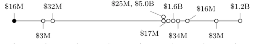
Toyota Motor Corp. (hereafter, Toyota), one of the world’s major automotive manufactures, implemented procedures to repair a gas pedal defect in its vehicles in Europe and Canada in late September 2009. Customer complaints claimed that the gas pedals in Toyota vehicles would become stuck, causing the vehicles to accelerate unexpectedly. Even though numerous US customers complained of the same problem, Toyota did not issue a recall in the US until January 2010. After Toyota issued the recall, the US Transportation Department began to investigate the company’s actions. They found that Toyota had known of the safety defects as early as September 2009 and yet did not report them until January 2010. As a result, Toyota had to pay several fines and penalties between April 2010 and March 2014 (as depicted in Figure 2).

10-2013 11-2013 05-2014

$5.1B $34M, $515M, $1.0B, $1.4B, $6.0B $280M

Figure 1: Timing of losses of JP Morgan due to the mis-selling of residential mortgage-backed securities

In summary, in the case of JP Morgan, from the initial loss of $US 5.1B, six more losses

1

For more examples we refer to the SAS OpRisk Global Data database, on which we give more details

in Section 4.

were settled and the accumulated losses, until May 2014, amounted up to $US 14.4B. In the case of Toyota, from the initial loss of $US 16.4M in April 2010, ten more losses were settled and the accumulated losses, until March 2014, totaled $US 8.0B. Figures 1 and 2 highlight that the initial triggering event does not contain all information about the future losses which may lead to very severe outcomes that extend over significant periods of time.

04-2010 10-2010 05-2011 11-2011 06-2012 12-2012 07-2013 01-2014

$16M

$3M

$32M $25M, $5.0B

$17M

$1.6B

$34M

$16M

$3M

$1.2B

Figure 2: Timing of losses of Toyota due to the sudden acceleration of vehicles attributed to the gas pedal’s failure to release

The main aim of this paper is to quantify the impact of prolonged losses from operational disruptions on multi-period risk measures. In particular, we use multi-period extensions of Value-at-Risk (VaR) and Expected Shortfall (ES) – two risk measures that are proposed in the literature and extensively used in practice. We develop a multi-period model of opera- tional risk which allows the integration of operational risk events that lead to multiple losses over time. Multi-period risk measurement is well established in the financial services sector (Pfister et al. 2015) and it has also been widely explored in the production and operations research literature (e.g., Tomlin 2006; Nickel et al. 2012). Especially in the manufacturing sector, multi-period risk measurement has equally if not more important implications, since investment decisions typically have longer time-horizons in capital-intensive industries. For instance, financing a new factory site is a decision in which return on investment tends to be measured in decades as opposed to loans issued by banks which typically mature in less than 10 years. Moreover, transaction costs for investing in new machinery are usually high and such assets are held for a long time. In order to achieve sustainable growth, firms in both industry sectors have to rely on risk models that take into account the extended planning periods and the costs arising from lead times (De Treville et al. 2014).

Using a comprehensive database of operational losses, we calibrate our model for the

financial and manufacturing industries. In a next step, we compare our model to a parsimo- nious LDA model and find that operational risk is significantly underestimated if the events leading to multiple losses are not accounted for appropriately. These results can have serious implications for firms’ capital planning and budgeting processes, since a misinterpretation of the underlying risk of a project can lead to suboptimal investment decisions.

The rest of this paper is organized as follows. In Section 2, we review the relevant literature. Section 3 elaborates on the model definition. Next, in Section 4, we describe the data, which is used in Section 5 to calibrate the model. The simulation setup, results from the simulations as well as structural results from the model are presented in Section 6.

Finally, in Section 7, we conclude with implications for theory and managerial practice, and discuss limitations and future research.

2. Literature Review

Our research is anchored in the operations–finance interface literature (Birge 2015; Miz- gier et al. 2015a; Zhao and Huchzermeier 2015). While the literature is rather scarce, there are a few papers that recognize the possibility of prolonged losses in operational risk.

Chernobai and Yildirim (2008) propose a shot-noise process to simulate the arrival of opera- tional disruptions triggered by an initial event. Under the assumption that the events decay exponentially or follow a power law, they found that a one-period VaR could be underestim- ated if multiple loss effects are neglected. Bardoscia and Bellotti (2011) introduce a dynamic operational risk model, which incorporates the evolution of the losses in time and takes into account different time-correlations among the processes. Guegan and Hassani (2013) study the possibility of multiple losses triggered by one event by capturing autocorrelation and large losses simultaneously.

Our approach broadens the results of existing studies in several directions. First, we

introduce a multi-period measure of operational risk which accommodates the prolonged

impact of aftershocks more appropriately. The application of multi-period risk measures

is especially desirable for capital allocation purposes (Pfister et al., 2015), in which the

evolution of risk during the lifespan of a project is essential. While the multi-period approach

is well established in the management of other types of risk (such as credit or market risk), it has not yet received such attention in the operational risk literature. Second, we do not impose any restrictions on the loss generating process. We fit and calibrate the distribution of the aftershocks of an event and explicitly model the length and severity of the loss chains.

Thus, if the data suggests a distribution of aftershocks that is not exponential, it can be readily incorporated into our general model formulation. Third, we empirically demonstrate the existence of differences in operational risk measures between the financial services and the manufacturing sector. In contrast to Chernobai and Yildirim (2008), we use data that spans the entire industry sectors which makes our results more generalizable.

In the remainder of this section, we first detail one- and multi-period approaches to risk modeling. Then we compare operational risk management practices in the financial and manufacturing industry sectors.

2.1. One and multi-period risk models

While various one-period risk measures such as Value-at-Risk (VaR) were proposed in the late 20th century, a rigorous analysis of the properties of such measures commenced with the seminal work of Artzner et al. (1999). They define a coherent risk measure to inhibit four desirable properties, in particular monotonicity, sub-additivity, positive homogeneity, and translation invariance. Later on, some authors proclaim a relaxation of the notions of sub-additivity and positive homogeneity to the notion of convexity (Föllmer and Schied, 2002), whereas others proclaim the use of spectral risk measures, which form a tightening of coherent risk measures (Acerbi, 2002).

From a mathematical viewpoint, all such one-period risk measures are a map from a

random variable (representing the risky cash flows, for instance the losses from operational

disruptions) to a real number (representing the risk). When lifting one-period risk measure-

ment to a multi-period setting, the input for the risk measure function becomes a stochastic

process (representing the cash flows of future periods). The output of multi-period risk

measures can either be a random process representing the (today unknown) risk in future

periods (see Pfister et al., 2015, for an overview), or a real number aggregating the risk

of all future periods into a single term (Frittelli and Scandolo, 2006; Artzner et al., 2007).

For practical purposes, the latter type of multi-period risk measures is more relevant. Melo et al. (2009) showed that this approach can be used to the facility location problem in which parameters change over time. Moreover, an overview of multi-period supply chain design decisions can be found in Klibi et al. (2010).

2.2. Operational risk measurement in financial services and manufacturing

In particular in the field of financial literature, operational risk measurement has received significant attention (Embrechts et al. 2003; De Fontnouvelle et al. 2006) and is closely followed in practice (Frachot et al. 2007; Chernobai et al. 2008). The main approach to quantifying operational risk is related to the calculation of VaR and Conditional VaR (CVaR) which is also termed Expected Shortfall (ES) by banks and insurance companies (Rockafellar and Uryasev 2002). One common method used to calculate VaR is the LDA which draws on the mathematics of actuarial science (Bühlmann 1970, Nešlehová et al. 2006, Chavez- Demoulin et al. 2015). Two input distributions are required for the LDA: the frequency and severity of operational losses. The typical applications of VaR and CVaR are in enterprise- wide risk management and capital planning (Jorion 2006). These quantile measures of operational risk are mainly set in a one-period framework. However, a few multi-period approaches to the measurement of operational risk have been proposed in the literature, relying on a simple time-scaling transformation of the one-period VaR (e.g., Bocker and Klüppelberg 2005). Kleindorfer and Li (2005) study a multi-period model for portfolio optimization with applications to the electric power sector.

Furthermore, there are a number of applications of VaR (both in one- and multi-period

settings) that can be found in the operations management literature. For instance, Cash

Flow at Risk is used to measure losses due to industrial activities (Turner 1996). The

most widespread industrial applications of VaR are in the context of inventory management

(Tapiero 2005). Luciano et al. (2003) formulate a VaR approach to inventory earnings in a

multi-period inventory model. Ahmed et al. (2007) study an extension of the classical multi-

period, single-item, linear cost inventory problem where the objective function is a coherent

risk measure (CVaR). This problem, also known as a newsvendor problem, has also been studied by Choi and Ruszczyński (2008) and Jammernegg and Kischka (2009). Mizgier et al.

(2015b) apply VaR to measure risk in complex supply chain networks. Zhang et al. (2009) study one- and multi-period optimal inventory control models with risk-averse constraints.

Another class of VaR models in inventory control has been proposed by Borgonovo and Peccati (2009) who offer a quantitative measurement of the similarity/discrepancy of policies reflecting different risk attitudes. In Borgonovo and Peccati (2011), the authors extend the proposed model and introduce a comprehensive approach to the sensitivity analysis of risk- coherent inventory models. A comprehensive overview of the current state of knowledge about the applications of VaR to supply chain risks can be found in Chiu and Choi (2013).

In this study different areas of supply chain management research are addressed, including single-echelon, multi-echelon supply chains, both in single and multi-period settings. In the context of firms’ industry affiliation, Mizgier et al. (2015a) investigate statistical properties of operational disruptions not only in the financial services but also in the manufacturing industry. The authors propose to manage operational risk through capital adequacy and/or process improvement contingent upon the risk event type and industry sector.

3. Model Specification

Building upon the insights from the literature in the previous section, we specify our model for estimating the risk from operational disruptions. To this end, first we need to define a loss process capturing the distribution of the losses. Afterward, we need to specify a risk measure that translates the loss process to an interpretable figure. In order to remain as general as possible, we do not impose any distributional assumption for our model in this section.

3.1. Loss process

The point of debarkation for our model relies on the observation that a significant portion

of operational risk losses cannot be characterized as being independent. Instead, as high-

lighted in the examples of Figures 1 and 2, there are triggering events which are followed

by a number of subsequent losses. In particular, the SAS OpRisk Global Data database characterizes a total amount of $US 735B as operational losses from single event, multiple losses (SEML) type. Given a total amount of operational risk losses of $US 2,901B, SEML type losses account for more than 25% of all losses in this database. As pointed out by Chernobai and Yildirim (2008), such SEML type losses do not occur independent in time and thus cannot be modeled by a traditional LDA model. Let l

be the total loss amount from operational risk of a firm incurred in period t and L

= ∑

t=1

l

be the cumulative loss until period T . We split the total loss into two classes with distinct stylized characteristics.

3.1.1. Single event, single loss (SESL)

SESL type events form the typical losses in operational risk. The main assumption is that both the frequency and the severity of the losses are identically and independently (iid) distributed, respectively. Let l

denote the total loss from such events in period t. Let F

denote the number of losses incurred in period t and S

denote the severity of the ith loss in period t.

Then, the total loss of all SESL type losses in period t is the sum of all losses occurring in the same period, i.e.,

l

=

Ft

∑

i=1

S

,

and the cumulative loss until period T is L

=

∑

t=1 Ft

∑

i=1

S

, (1)

where F

∼ iid for all t and S

∼ iid for all t and i.

3.1.2. Single event, multiple losses (SEML)

In this case, we relax the iid assumption for the loss frequency distribution. Instead

of modeling the amount of losses incurred in each period directly, we consider triggering

events. Each triggering event is the head of an event chain that can induce losses in a

certain number of periods (the length of the chain). Let the random variable E

denote the

number of triggering events in period t (i.e., event chains starting in period t) and let e

,

1 2 3 4 5 6 e

e

e

e

e

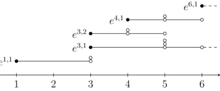
Figure 3: SEML frequency modeling. This figure illustrates the approach of modeling the frequency of SEML losses. The different periods of the model are denoted on the x-axis. The black dots represent triggering events e. Each triggering event can induce several losses in subsequent years, which are depicted by white dots.

i = 1, . . . , E

, denote the triggering events in period t. The number of subsequent periods after a triggering event in which losses are induced by the event (i.e., the length of the chain) is specific to the event and denoted by the random variable L

. Finally, the random variable F

, l = 0, . . . , L

, denotes number of losses induced by event e

in the lth period of the event chain (i.e., in period t + l) and the random variable S

, j = 1, . . . , F

, denotes the severity of the jth loss of that event chain in period t + l.

Equipped with the above notation, the cumulative loss from all SEML type losses up to period T can be computed as

L

=

∑

t=0 E^t

∑

i=1

min{L

∑

F_l^t,i

∑

j=1

S

, (2)

where E

∼ iid, L

∼ iid, F

∼ iid, and S

∼ iid for all t, i, l, and j, respectively. The minimum operator in the third summation ensures that only losses that occur until period T are counted in equation (2).

Figure 3 illustrates this approach. Consider, for instance, the second triggering event in

period 3, e

. The event induces losses in the two subsequent periods, i.e., L

= 2. In

the first subsequent period (period 4), there are two losses, i.e., F

= 2, in the second

subsequent period (period 5), there is one loss, i.e., F

= 1. The first white dot to the

right of the black dot of e

represents the first loss in period 4, S

, and the dot above it

represents the second loss in period 4, S

. The rightmost dot in the line represents the loss

in period 5, S

.

Altogether, the total loss incurred until period T is the sum of all SESL type losses and all SEML type losses in period T , i.e., L

= L

+ L

.

3.2. Risk measures

Once a proper loss process has been specified, the next step is to find an adequate risk measure. As above, let L = (L

)

be the cumulative loss process. While single period risk measures would consider only the next periods loss L

, we use the following two multi- period risk measures with horizon T and discount rate r (cf. the Appendix of Pfister et al., 2015):

VaR

(L) = VaR

(L

) + 1

1 + r (VaR

(L

) − VaR

(L

)) + . . . +

+ 1

(1 + r)

(VaR

(L

) − VaR

(L

))

=

T−1

∑

t=1

( r

(1 + r)

VaR

(L

) )

+ r

(1 + r)

VaR

(L

) ES

(L) = ES

(L

) + 1

1 + r (ES

(L

) − ES

(L

)) + . . . +

+ 1

(1 + r)

(ES

(L

) − ES

(L

))

=

T−1

∑

t=1

( r

(1 + r)

ES

(L

) )

+ r

(1 + r)

ES

(L

)

Let us briefly illustrate the motivation for the two multi-period risk measures by means of the latter. For each period t = 1, . . . , T , there is a certain capital requirement ES

(L

) which depends on the accumulated losses up to that period. However, not all the capital ES

(L

) needs to be reserved today. Today, only ES

(L

) needs to be available. In the next period, ES

(L

) needs to be available so on average an additional capital of ES

(L

) − ES

(L

) will be required. The present value of this additional capital is added to today’s risk. One period later, an additional capital of ES

(L

) − ES

(L

) will be required. Again, the present value is added to today’s risk. This process iterates until the time horizon T is reached.

Using such a multi-period risk measure is decisive for many capital allocation applications,

in which the time structure of the required risk capital during the lifespan of a project may vary.

4. Data

In order to calibrate the above model, our primary source is the SAS OpRisk Global Data database. This database is one of the largest, most comprehensive, and most accurate repository of information on publicly reported operational losses in excess of US$ 100,000 (SAS 2014). As of September 2014, the database has comprised more than 31,000 operational loss events covering all industry sectors globally. Among the information provided for each loss event are date of loss, loss severity, name of firm, industry of firm, and a classification on whether it is a SESL or SEML type loss. In the latter case, there is a code assigned to each triggering event so that subsequent losses can be related to it.

We split our database into four subsamples, namely SESL and SEML type losses in two separate industry sectors: financial services and manufacturing. This resulted in 20,880 observations that we used in our analysis. These observations stem from 6,397 different firms from the financial services sector and from 3,897 different firms from the manufacturing sector. The loss severities have been scaled using the 2014 Consumer Price Index. All figures are represented in US$ million.

4.1. Descriptive statistics—Single event single losses

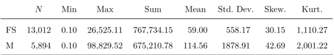
The SESL severity distributions are characterized by relatively low mean values and high skewness and kurtosis pointing to heavy-tailed distributions. This observation is consistent with other empirical studies (e.g., Chavez-Demoulin et al. 2006). As Table 1 reports, higher mean and higher maximum values can be observed in the manufacturing than in the financial industry.

4.2. Descriptive statistics—Single event multiple losses

There are 1,136 different SEML triggering events recorded in the database. Each trigger-

ing event induced several losses. Therefore, when aggregating, we wind up with 2,905 losses

Table 1: Descriptive statistics of SESL in financial services (FS) and manufacturing (M)

N Min Max Sum Mean Std. Dev. Skew. Kurt.

FS 13,012 0.10 26,525.11 767,734.15 59.00 558.17 30.15 1,110.27 M 5,894 0.10 98,829.52 675,210.78 114.56 1878.91 42.69 2,001.22

of which 1,160 losses belong to the financial services sector and 814 to the manufacturing sector. The remaining 931 losses belong to the other sectors such as mining, retail trade, construction, etc. and have been excluded from the analysis. As summarized in Table 2, the mean severity in both sectors is higher than in the SESL case, whereas the skewness and kurtosis are lower. There are 480 different firms from the financial services and 326 different firms from the manufacturing sector in the SEML data sample.

Table 2: Descriptive statistics of SEML in financial services (FS) and manufacturing (M)

N Min Max Sum Mean Std. Dev. Skew. Kurt.

FS 1,160 0.10 27,009.08 348,031.14 300.03 1,318.95 11.11 173.57 M 814 0.11 26,433.42 179,162.10 220.10 1,315.27 15.77 281.19

5. Model calibration

In order to be able to compare our model with a traditional LDA model, we estimate the multi-period risk measures for two different model specifications. The first one is a traditional SESL only model (designated SESL only model). This model assumes that all losses are of SESL type and all distributions are fitted using historical losses from both SESL and SEML types. Notice that this model is identical to a traditional LDA model.

The second model specification (designated SESL plus SEML model) includes SESL and SEML type losses separately. Here we fit the distributions of the loss process for SESL events and SEML events separately. The total loss is the sum of the losses of SESL and SEML type.

We fitted the following distributions of our operational risk model in both industry

sectors (SESL only and SESL plus SEML model):

1. Yearly frequency of operational disruptions F (discrete) 2. Severity of operational disruptions S (continuous)

Additionally, in the SESL plus SEML model, we fitted the following distributions:

3. Yearly frequency of triggering events E (discrete)

4. Length of the period of subsequent losses after a triggering event in years L (discrete) For discrete distributions, we calibrated the parameters for Binomial, Negative binomial, and Poisson distributions. For continuous distributions, we calibrated the parameters for Beta, Birnbaum–Saunders, Exponential, Extreme value, Gamma, Generalized extreme value, Gen- eralized Pareto, Inverse Gaussian, Logistic, Log-logistic, Lognormal, Nakagami, Normal, Rayleigh, Rician, t location-scale, and Weibull distributions. We rank each distribution according to the Bayesian information criterion

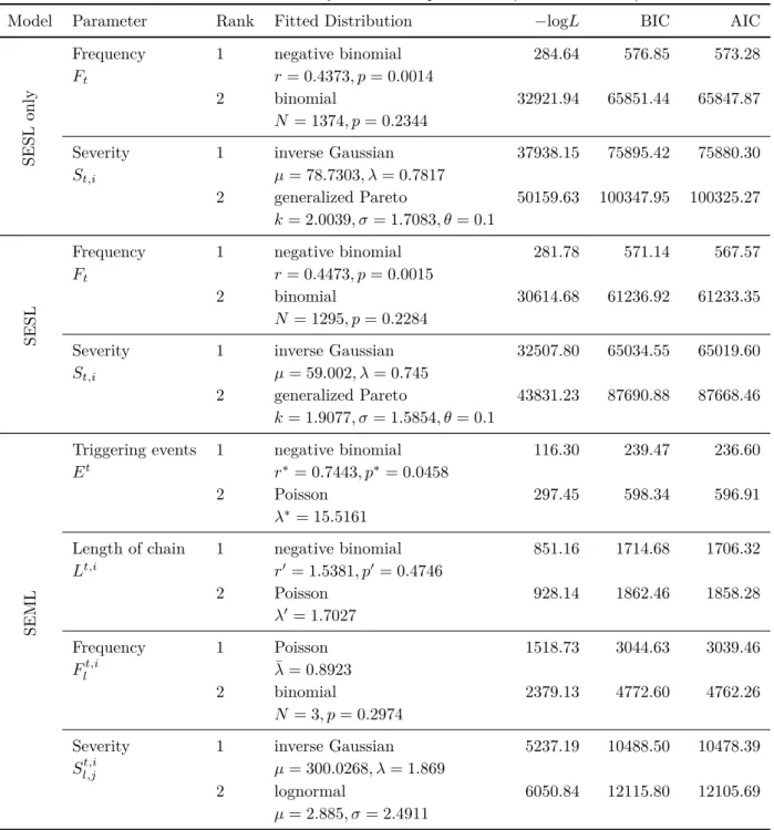
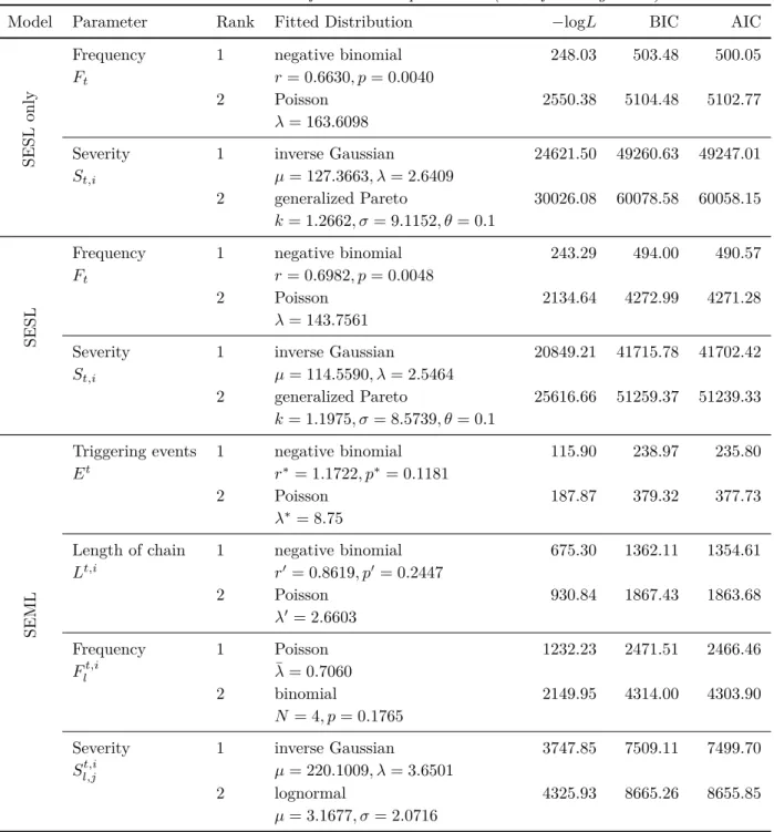
. Table 3 reports upon the best-fitting distribution and second best fitting distribution and the calibrated parameters for the fin- ancial industry sector. Table 4 reports upon the same results for the manufacturing in- dustry sector. In both industry sectors, the best fitting distributions are the same for all parameters—Inverse Gaussian for severity, Poisson for frequency in the SEML model, and negative binomial in all other instances. Our choice of distributions is in line with the guidance provided by the relevant literature (Klugman et al. 2012). Moreover, the existing applications in the financial services industry further confirm the validity of our approach (Boucher et al. 2008; McNeil et al. 2015).

6. Results

Note that while we are eventually interested in calculating the risk on a firm level, our calibration of the number of yearly SESL losses (SEML triggering events) was on an industry sector level. Hence, we alter our model from Section 3.1 in such a way that instead of of taking the distribution for the frequency F

(SESL) and for the triggering events E

from Section 5 directly, we use a compound distribution Bin(N

, 1/n) for these distributions,

2

A ranking according to the Akaike information criterion or Log Likelihood does not alter the best fit.

Table 3: Fit and calibration of distribution parameters (Financial sector).

Model Parameter Rank Fitted Distribution −logL BIC AIC

SESL only

Frequency 1 negative binomial 284.64 576.85 573.28

F

r = 0.4373, p = 0.0014

2 binomial 32921.94 65851.44 65847.87

N = 1374, p = 0.2344

Severity 1 inverse Gaussian 37938.15 75895.42 75880.30

S

µ = 78.7303, λ = 0.7817

2 generalized Pareto 50159.63 100347.95 100325.27 k = 2.0039, σ = 1.7083, θ = 0.1

SESL

Frequency 1 negative binomial 281.78 571.14 567.57

F

r = 0.4473, p = 0.0015

2 binomial 30614.68 61236.92 61233.35

N = 1295, p = 0.2284

Severity 1 inverse Gaussian 32507.80 65034.55 65019.60

S

µ = 59.002, λ = 0.745

2 generalized Pareto 43831.23 87690.88 87668.46

k = 1.9077, σ = 1.5854, θ = 0.1

SEML

Triggering events 1 negative binomial 116.30 239.47 236.60

E

r

= 0.7443, p

= 0.0458

2 Poisson 297.45 598.34 596.91

λ

= 15.5161

Length of chain 1 negative binomial 851.16 1714.68 1706.32

L

r

= 1.5381, p

= 0.4746

2 Poisson 928.14 1862.46 1858.28

λ

= 1.7027

Frequency 1 Poisson 1518.73 3044.63 3039.46

F

λ ¯ = 0.8923

2 binomial 2379.13 4772.60 4762.26

N = 3, p = 0.2974

Severity 1 inverse Gaussian 5237.19 10488.50 10478.39

S

µ = 300.0268, λ = 1.869

2 lognormal 6050.84 12115.80 12105.69

µ = 2.885, σ = 2.4911

Table 4: Fit and calibration of distribution parameters (Manufacturing sector).

Model Parameter Rank Fitted Distribution −logL BIC AIC

SESL only

Frequency 1 negative binomial 248.03 503.48 500.05

F

r = 0.6630, p = 0.0040

2 Poisson 2550.38 5104.48 5102.77

λ = 163.6098

Severity 1 inverse Gaussian 24621.50 49260.63 49247.01

S

µ = 127.3663, λ = 2.6409

2 generalized Pareto 30026.08 60078.58 60058.15

k = 1.2662, σ = 9.1152, θ = 0.1

SESL

Frequency 1 negative binomial 243.29 494.00 490.57

F

r = 0.6982, p = 0.0048

2 Poisson 2134.64 4272.99 4271.28

λ = 143.7561

Severity 1 inverse Gaussian 20849.21 41715.78 41702.42

S

µ = 114.5590, λ = 2.5464

2 generalized Pareto 25616.66 51259.37 51239.33

k = 1.1975, σ = 8.5739, θ = 0.1

SEML

Triggering events 1 negative binomial 115.90 238.97 235.80

E

r

= 1.1722, p

= 0.1181

2 Poisson 187.87 379.32 377.73

λ

= 8.75

Length of chain 1 negative binomial 675.30 1362.11 1354.61

L

r

= 0.8619, p

= 0.2447

2 Poisson 930.84 1867.43 1863.68

λ

= 2.6603

Frequency 1 Poisson 1232.23 2471.51 2466.46

F

λ ¯ = 0.7060

2 binomial 2149.95 4314.00 4303.90

N = 4, p = 0.1765

Severity 1 inverse Gaussian 3747.85 7509.11 7499.70

S

µ = 220.1009, λ = 3.6501

2 lognormal 4325.93 8665.26 8655.85

µ = 3.1677, σ = 2.0716

where N

is the respective industry-wide frequency F

or E

and n is the total numbers of firms in the respective industry (n = 6397 and n = 3897 for the financial and manufacturing sector, respectively). This assumes that each firm in an industry is equally prone to the losses (given the regulatory-driven unification of risk management practices, this is a fairly justified assumption (De Luna-Martinez and Rose 2003), which could however be altered by adjusting the probability parameter 1/n in the binomial distribution).

In the following, we use two different approaches to derive estimates for the multi-period risk measures as detailed in Section 3.2. The first is Monte Carlo simulations, the second builds upon structural results derived from our model of Section 3.1. In both approaches, we use a relatively high confidence level α = 99.9%, which is predominant with respect to operational losses.

6.1. Monte Carlo simulations

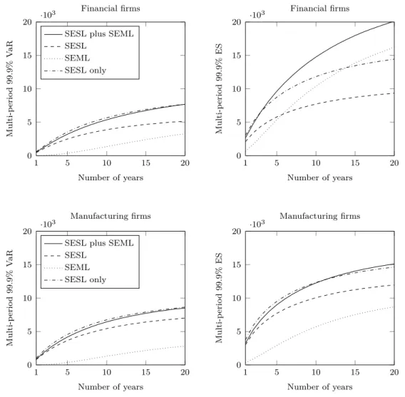
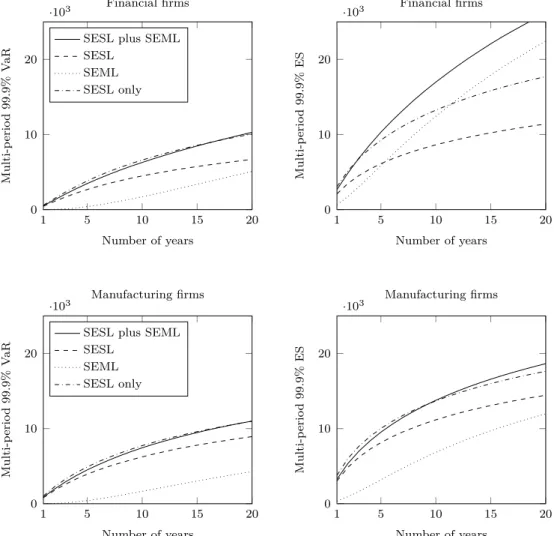
Since high impact losses are relatively scarce, we use Monte Carlo simulations with 500 million iterations to compute our risk measures with the calibrated model and a time- horizon of 20 years. Figure 4 displays the multi-period VaR and ES for financial and man- ufacturing firms with an annual discount rate of 5%.

The dash-dotted line in each graph represents the total risk for the traditional SESL only model, whereas the solid line rep- resents the total risk for the SESL plus SEML model. Furthermore, we display the SESL component (dashed line) and SEML component (dotted line) of the SESL plus SEML model.

With respect to the industry sector, the level of operational risk both the financial and manufacturing industry are comparable. When comparing the SESL plus SEML model to the SESL only model, our results show that a parsimonious LDA approach captures the risk (both measured with VaR and ES) surprisingly well in the manufacturing sector for all time horizons. The same holds true when using VaR as risk measure in the financial sector.

However, this general picture changes when considering ES in the financial sector. Consid- ering the upper right graph in Figure 4, we infer that the SESL only model substantially underestimates the true risk for time horizons exceeding 4 years.

3

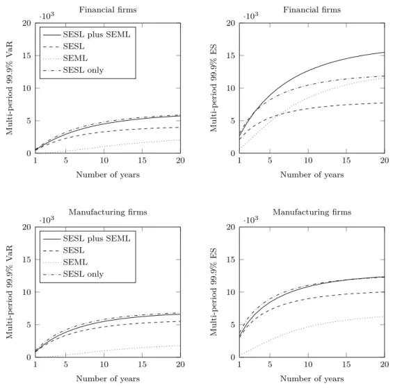
The results with different discount rates are displayed in Figures A.1 and A.2 in the Appendix.

5 10 15 20 0

5 10 15 20 ·10³

1

Number of years

Multi-period99.9%VaR

Financial firms

SESL plus SEML SESL

SEML SESL only

5 10 15 20

0 5 10 15 20 ·10³

1

Number of years

Multi-period99.9%ES

Financial firms

5 10 15 20

0 5 10 15 20 ·10³

1

Number of years

Multi-period99.9%VaR

Manufacturing firms

SESL plus SEML SESL

SEML SESL only

5 10 15 20

0 5 10 15 20 ·10³

1

Number of years

Multi-period99.9%ES

Manufacturing firms

Figure 4: Multi-period VaR and ES. The four graphs in this figure display the multi-period VaR (left) and

multi-period ES (right) for financial firms (top) and manufacturing firms (bottom). In each graph, we display

the risk of the total (SESL plus SEML) loss process L

(solid line), the risk of the SESL process L

(dashed line), the risk of the SEML process L

(dotted line), and the total risk under the assumption

of SESL losses only (dash-dotted line). All risk measures are computed using a 99.9% confidence level and

a discount rate of r = 5%. All values are expressed in US$ million.

5 10 15 20 0

0.2 0.4 0.6 0.8 1

1

Number of years

ProportionofSEMLRisk

Multi-period 99.9% VaR

Financial Manufacturing

5 10 15 20

0 0.2 0.4 0.6 0.8 1

1

Number of years

ProportionofSEMLRisk

Multi-period 99.9% ES

Financial Manufacturing 0

0.2 0.4 0.6 0.8 1

ProportionofSESLRisk

Multi-period 99.9% VaR

0 0.2 0.4 0.6 0.8 1

ProportionofSESLRisk

Multi-period 99.9% ES

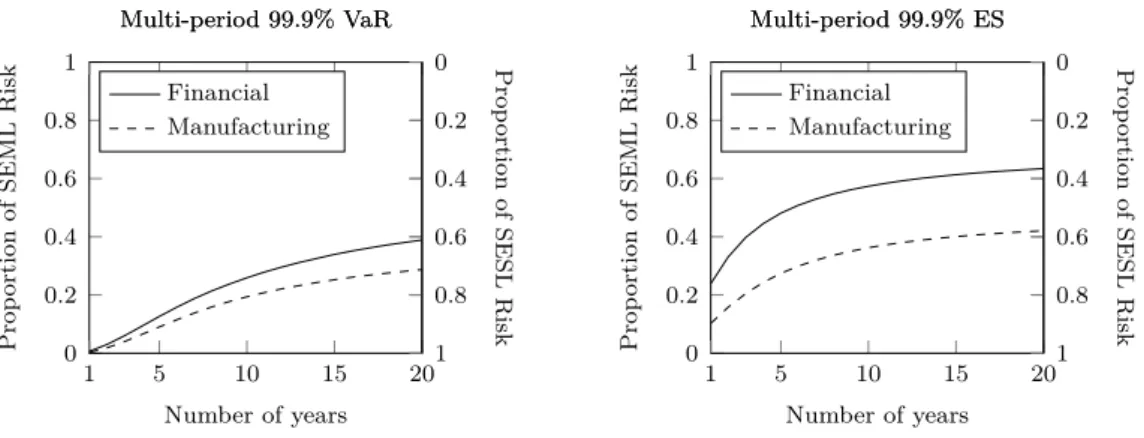
Figure 5: Proportion of SEML and SESL risk. This figure displays the proportion of risk induced by the SEML and SESL losses on the risk induced by the total losses for financial firms (solid line) and manufacturing firms (dashed line). Risk is measured as multi-period VaR (left) and multi-period ES (right).

All risk measures are computed using a 99.9% confidence level and a discount rate of r = 5%.

To gain more insight, we partition the SESL plus SEML risk into its two components, the SESL risk and the SEML risk and plot these proportions in Figure 5. For instance, the solid line in the left plot shows that when considering the first year, only 0.7% of the total VaR stems from SEML losses. When considering twenty years, this figure increases to 38.9%. Generally, the proportion of SEML risk is higher in the financial industry sector than in the manufacturing sector. The most pronounced influence of SEML losses can be observed for the ES in the financial sector when considering time horizons of 4 years and more, when the proportion of the SEML component reaches 44.5–63.4%.

6.2. Structural results

In this section, we analytically compute the first four moments of the loss of SESL and

SEML type. Afterward, we compare analytical VaR and ES estimates using both normal

and Johnson distributions to the VaR and ES computed via Monte Carlo simulations in the

previous section.

6.2.1. SESL

With the adaption to a firm level described in Section 6, the cumulative loss from SESL events from Equation (1) can be expressed as

L

=

∑

t=1 Ft

∑

i=1

S

,

where S

∼ InvGaussian(µ, λ) and F

∼ Bin(N

,

) with N

∼ NegBin(r, p) are the fitted distributions with the respective parameters from Section 5. The probability generating function ψ

of the compound random variable F

can be computed as

ψ

(u) = ψ

(ψ

(u)) =

( 1 − p

1 − p((1 −

) +

u) )

, cf. Gut (1991), Theorem 5.1. Using ψ

(u), the characteristic function φ

t

of L

is φ

T

(u) = ( ψ

(

φ

(u) ))

, where φ

(u) = exp

(

λ µ

( 1 − √

1 −

))

is the characteristic function of S

. Comput- ing the moments E [

(L

)

]

= i

[

du^k

φ

T

(u)

]

u=0

yields µ(L

) = T µpr

n (1 − p) σ

(L

) = T µ

pr

λn (1 − p) + T µ

pr (n + p − np) n

(1 − p)

Skew(L

) =

T )

(

λ²n(1−p)

+

+

) Kurt(L

) =

T )

(

λn³(1−p)³

−

(

)

λ³n(1−p)

+

−

λ²n²(1−p)²

+

)

Using these moments, we compute two different analytic estimates for the VaR and ES.

The first ones are the canonical estimates assuming a normal distribution and are computed as

VaR

(L

) = µ(L

) + σ(L

) · Φ

(α)

ES

(L

) = µ(L

) + σ(L

) · ϕ(Φ

(α)) 1 − α ,

in which Φ

( · ) and ϕ( · ) denote the inverse cdf and pdf of the standard normal distribution, respectively. The second measures take the skewness and kurtosis of the loss distribution into account using the Johnson (1949) SL translation. This translation transforms a continuous random variable Z into the normalized form Y = a + b · ln (

d

) and the parameters a, b, c, and d can be estimated from the first four moments of the random variable Z. Simonato (2011) derives the following analytical formulas for VaR and ES:

VaR

(L

) = µ(L

) + σ(L

) · (

c + d · exp

( Φ

(α) − a b

))

ES

(L

) = µ(L

) + σ(L

) ·

(

)

1−α

,

where K = a + b · ln

(

− c

) − b · ln(d).

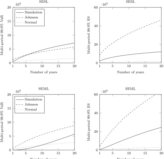
The two upper graphs in Figure 6 compare the two analytic VaR and ES estimates with the results from our previous Monte Carlo simulation for the financial firms. Clearly, the normal estimator heavily underestimates both risk measures, as it does not take the high skewness and kurtosis of the loss distribution into account. The Johnson estimate, however, works reasonable well for the VaR estimate at an 99.9% level. Yet, it overestimates the true risk according to the ES measure by a factor of 2–4.

6.2.2. SEML

After switching sums and changing variables of the second sum, Equation (2) for the SEML process becomes

L

=

∑

t=0

min{

∑

E^t

∑

i=1 F_l^t,i

∑

j=1

S

,

where S

∼ InvGaussian(µ, λ), F

∼ Poisson(¯ λ), E

∼ Bin(N

,

) with F

∼ NegBin(r

, p

)

and L

∼ NegBin(r

, p

) are the fitted distributions with the respective parameters from

Section 5. To compute the first four moments of L

, we use Equations (32a–d) from

Grubbström and Tang (2006) for each summation iteratively. These equations provide for-

mulas for computing the moments of a random sum of random variables. However, the

5 10 15 20 0

5 10 15 20 ·10³

1

Number of years

Multi-period99.9%VaR

SESL

Simulation Johnson Normal

5 10 15 20

0 20 40 60 ·10³

1

Number of years

Multi-period99.9%ES

SESL

5 10 15 20

0 5 10 15 20 ·10³

1

Number of years

Multi-period99.9%VaR

SEML

Simulation Johnson Normal

5 10 15 20

0 20 40 60 ·10³

1

Number of years

Multi-period99.9%ES

SEML

Figure 6: Multi-period VaR and ES. The four graphs in this figure display the multi-period VaR (left) and

multi-period ES (right) for SESL (top) and SEML (bottom) losses of financial firms. In each graph, we

display the simulated risk measures (solid line), the risk according to the Johnson estimator (dashed line),

and the risk according to a normal mean–variance estimator (dotted line). All risk measures are computed

using a 99.9% confidence level and a discount rate of r = 5%. All values are expressed in US$ million.

second and the third summation need special care. The third is a random sum of a com- pound distribution E

. The moments of E

, however, can be computed using the probability generating functions similarly to the SESL case. The second is a random sum of a trun- cated random variable. Since L

is a discrete random variable and the truncation is from above, the moments of min { L

, t } can be computed directly using the discrete probabilities P (L

= x), x = 0, . . . , t.

Similar to the SESL case, we compute the normal and Johnson VaR and ES, respectively, with the first four moments of L

for the financial firms. The results are plotted in the two lower graphs in Figure 6. In general, the analytic Johnson VaR and ES overestimate the true risk, whereas the analytic normal ES underestimates the true risk. In the case of the normal VaR, the true risk is overestimated for short time horizons (up to 9 years) and underestimated for longer time horizons.

6.3. Implications for capital allocation

The different outcomes for the risk of the total loss process (cf. Figure 4) can have serious implications for the capital allocation in firms with different lines of business. Generally, capital allocations principles, such as gradient allocation introduced by Tasche (2004), can be used to compute the marginal capital requirement of each line of business. A multi- objective capital allocation problem was proposed by Mizgier and Pasia (2015). Buch and Dorfleitner (2008) introduce the notation of coherent capital allocation and note that it is desirable to use a coherent risk measure in the allocation principle. Therefore, let A

be an expected shortfall-based allocation principle so that ∑

n=1

A

= ES(L), where L denotes the loss process of the entire firm. In particular, gradient allocation is given by

A

= lim

h→0

ES( ∑

n̸=m

L

+ hL

) − ES( ∑

n̸=m

L

)

h , (3)

where L

denotes the total loss of the nth line of business. To illustrate the potential impacts,

consider a large automotive manufacturing group. Such groups typically have two major

lines of business, the traditional manufacturing arm and a financial services arm. When

allocating operational risk capital to the two arms, it becomes evident from Equation (3)

that a precise estimation of the operational loss processes for each arm is critical. Now, as illustrated in Section 6.1, a traditional SESL only process may underestimate the true risk especially for the financial services arm. In turn, the financial services arm is being allocated more risk capital than appropriate.

7. Conclusions, limitations and future research

Our research has important contributions both to the literature and managerial prac- tice. To our knowledge this is the first study to formally propose a multi-period model for operational risk. As opposed to other studies which tackle the issue of prolonged losses (e.g., Chernobai and Yildirim 2008), we do not assume any structural model formulation or suggest a priori any distributional loss properties. Our contribution to the literature is also to provide analytical estimates of VaR and ES using both normal and Johnson dis- tributions. Therefore, our model generalizes the existing approaches and extends them to a multi-period setting. Moreover, we show that, due to the possibility of prolonged dis- ruptions, multi-period risk measures reveal the true impact of multiple losses over longer planning horizons. Our approach can be utilized by firms in the financial services and in the manufacturing sector to better manage their capital allocation decisions.

By investigating a large dataset of operational disruptions, we observe substantial dif- ferences in the reported risk figures between the two industry sectors. The proportion of SEML risk is generally higher in financial services than in manufacturing firms. Moreover, the impact of SEML losses becomes particularly relevant when risk calculations are exten- ded over several years. Driven by the insights of our model, risk managers can assess the impact of prolonged losses on their long-term strategic decisions.

As computational power increases, we could run 500 million Monte Carlo simulations in

an acceptable run-time (approximately six hours on a personal computer). By doing so, we

could circumvent the problem of small samples for heavy-tailed distributions, making our

results more robust. We demonstrate that operational risk can be severely underestimated

when SEML losses are treated in the same manner as SESL losses, which is the current best

practice. This implication is particularly important for policy-makers and regulators aiming to impose more realistic capital requirements on the regulated firms.

The limitation of our study lies in the granularity of data resulting from the event recording mechanism. As operational losses are rather infrequent, we had to aggregate the losses into yearly counts, leading to the loss of some information. Nonetheless, since our model is mainly used for long-term capital planning, this limitation does not affect the degree to which our results can be generalized.

Future research could focus on incorporating the multi-period view of operational risk into the general capital allocation framework. The aggregation of operational risk with other types of risk in the multi-period setting is also an interesting research path to be explored in the future. Our proposed method directly impacts the firms’ capital planning activities, but it is also noteworthy that regulators could benefit from this approach as well. The design of stress-tests, which include our proposed methodology in order to support the sustainable growth of the regulated firms, is a promising future research path.

References

Acerbi, C. (2002). Spectral measures of risk: A coherent representation of subjective risk aversion. Journal of Banking & Finance, 26:1505–1518.

Ahmed, S., Cakmak, U., and Shapiro, A. (2007). Coherent risk measures in inventory problems. European Journal of Operational Research, 182(1):226–238.

Ames, M., Schuermann, T., and Scott, H. S. (2015). Bank capital for operational risk: A tale of fragility and instability. Journal of Risk Management in Financial Institutions, 8(3):227–243.

Artzner, P., Delbaen, F., Eber, J.-M., and Heath, D. (1999). Coherent measures of risk. Mathematical Finance, 9(3):203–228.

Artzner, P., Delbaen, F., Eber, J.-M., Heath, D., and Hyejin, K. (2007). Coherent multiperiod risk adjusted values and Bellman’s principle. Annals of Operations Research, 152(1):5–22.

Aue, F. and Kalkbrener, M. (2006). LDA at work: Deutsche Bank’s approach to quantifying operational risk. Journal of Operational Risk, 1(4):49–93.

Bardoscia, M. and Bellotti, R. (2011). A dynamical approach to operational risk measurement. The Journal

of Operational Risk, 6(1):3–19.

Birge, J. R. (2015). OM Forum–Operations and Finance Interactions. Manufacturing & Service Operations Management, 17(1):4–15.

Bocker, K. and Klüppelberg, C. (2005). Operational VaR: a closed-form approximation. RISK Magazine, 18(12):90–93.

Borgonovo, E. and Peccati, L. (2009). Financial management in inventory problems: Risk averse vs risk neutral policies. International Journal of Production Economics, 118(1):233–242.

Borgonovo, E. and Peccati, L. (2011). Finite change comparative statics for risk-coherent inventories.

International Journal of Production Economics, 131(1):52–62.

Boucher, J.-P., Denuit, M., and Guillen, M. (2008). Models of insurance claim counts with time dependence based on generalisation of Poisson and negative binomial distributions. Variance, 2(1):135–162.

Buch, A. and Dorfleitner, G. (2008). Coherent risk measures, coherent capital allocations and the gradient allocation principle. Insurance: Mathematics & economics, 42:235–242.

Bühlmann, H. (1970). Mathematical Methods in Risk Theory. Grundlehren der mathematischen Wis- senschaft: A series of comprehensive studies in mathematics. Springer.

Chavez-Demoulin, V., Embrechts, P., and Hofert, M. (2015). An extreme value approach for modeling operational risk losses depending on covariates. Journal of Risk and Insurance.

Chavez-Demoulin, V., Embrechts, P., and Nešlehová, J. (2006). Quantitative models for operational risk:

extremes, dependence and aggregation. Journal of Banking & Finance, 30(10):2635–2658.

Chernobai, A. and Yildirim, Y. (2008). The dynamics of operational loss clustering. Journal of Banking &

Finance, 32(12):2655–2666.

Chernobai, A. S., Rachev, S. T., and Fabozzi, F. J. (2008). Operational risk: a guide to Basel II capital requirements, models, and analysis, volume 180. John Wiley & Sons.

Chiu, C.-H. and Choi, T.-M. (2013). Supply chain risk analysis with mean-variance models: a technical review. Annals of Operations Research, pages 1–19.

Choi, S. and Ruszczyński, A. (2008). A risk-averse newsvendor with law invariant coherent measures of risk.

Operations Research Letters, 36(1):77–82.

Chorafas, D. N. (2004). Five models by the Basel Committee for computation of operational risk. In Chorafas, D. N., editor, Operational Risk Control with Basel II, pages 141–162. Butterworth-Heinemann, Oxford.

De Fontnouvelle, P., De Jesus-Rueff, V., Jordan, J. S., and Rosengren, E. S. (2006). Capital and risk: New evidence on implications of large operational losses. Journal of Money, Credit, and Banking, 38(7):1819–

1846.

De Luna-Martinez, J. and Rose, T. A. (2003). International survey of integrated financial sector supervision,

volume 3096. World Bank Publications.

De Treville, S., Bicer, I., Chavez-Demoulin, V., Hagspiel, V., Schürhoff, N., Tasserit, C., and Wager, S.

(2014). Valuing lead time. Journal of Operations Management, 32(6):337–346.

Embrechts, P., Furrer, H., and Kaufmann, R. (2003). Quantifying regulatory capital for operational risk.

Derivatives Use, Trading & Regulation, 9(3):217–233.

Föllmer, H. and Schied, A. (2002). Convex measures of risk and trading constraints. Finance and Stochastics, 6(4):429–447.

Frachot, A., Moudoulaud, O., and Roncalli, T. (2007). Loss distribution approach in practice. In Ong, M., editor, The Basel Handbook: A Guide for Financial Practitioners, pages 527–554. Risk Books, London, UK.

Frittelli, M. and Scandolo, G. (2006). Risk measures and capital requirements for processes. Mathematical Finance, 16(4):589–612.

Grubbström, R. W. and Tang, O. (2006). The moments and central moments of a compound distribution.

European Journal of Operational Research, 170:106–119.

Guegan, D. and Hassani, B. (2013). Using a time series approach to correct serial correlation in operational risk capital calculation. The Journal of Operational Risk, 8(3):31–56.

Gut, A. (1991). An Intermediate Course in Probability. Springer, New York.

Jammernegg, W. and Kischka, P. (2009). Risk preferences and robust inventory decisions. International Journal of Production Economics, 118(1):269–274.

Johnson, N. L. (1949). System of frequency curves generated by methods of translation. Biometrika, 36:149–176.

Jorion, P. (2006). Value at Risk, 3rd Ed.: The New Benchmark for Managing Financial Risk. McGraw-Hill Education.

Kleindorfer, P. R. and Li, L. (2005). Multi-period VaR-constrained portfolio optimization with applications to the electric power sector. The Energy Journal, 26(1):1–26.

Klibi, W., Martel, A., and Guitouni, A. (2010). The design of robust value-creating supply chain networks:

a critical review. European Journal of Operational Research, 203(2):283–293.

Klugman, S., Panjer, H., and Willmot, G. (2012). Loss Models: From Data to Decisions, 4th Edition. John Wiley & Sons, New York.

Luciano, E., Peccati, L., and Cifarelli, D. M. (2003). VaR as a risk measure for multiperiod static inventory models. International Journal of Production Economics, 81–-82:375–384.

McNeil, A. J., Frey, R., and Embrechts, P. (2015). Quantitative Risk Management: Concepts, Techniques and Tools. Princeton University Press. Oxfordshire, UK.

Melo, M. T., Nickel, S., and Saldanha-da Gama, F. (2009). Facility location and supply chain management

– a review. European Journal of Operational Research, 196(2):401–412.

Mizgier, K. J., Hora, M., Wagner, S. M., and Jüttner, M. P. (2015a). Managing operational disrup- tions through capital adequacy and process improvement. European Journal of Operational Research, 245(1):320–332.

Mizgier, K. J. and Pasia, J. M. (2015). Multiobjective optimization of credit capital allocation in financial institutions. Central European Journal of Operations Research.

Mizgier, K. J., Wagner, S. M., and Jüttner, M. P. (2015b). Disentangling diversification in supply chain networks. International Journal of Production Economics, 162:115–124.

Nešlehová, J., Embrechts, P., and Chavez-Demoulin, V. (2006). Infinite mean models and the LDA for operational risk. Journal of Operational Risk, 1(1):3–25.

Nickel, S., Saldanha-da Gama, F., and Ziegler, H.-P. (2012). A multi-stage stochastic supply network design problem with financial decisions and risk management. Omega, 40(5):511–524.

Pfister, T., Utz, S., and Wimmer, M. (2015). Capital allocation in credit portfolios in a multi-period setting:

a literature review and practical guidelines. Review of Managerial Science, 9(1):1–32.

Rockafellar, R. T. and Uryasev, S. (2002). Conditional value-at-risk for general loss distributions. Journal of Banking & Finance, 26(7):1443–1471.

SAS (2014). SAS OpRisk Global Data. SAS Institute. Retrieved from

http://www.sas.com/resources/product-brief/sas-oprisk-globaldata-brief.pdf on November 6, 2014.

Simonato, J.-G. (2011). The performance of Johnson distributions for computing value at risk and expected shortfall. Journal of Derivatives, 19(1):7–24.

Tapiero, C. S. (2005). Value at risk and inventory control. European Journal of Operational Research, 163(3):769–775.

Tasche, D. (2004). Allocating portfolio economic capital to sub-portfolios. In Dev, A., editor, Economic Capital: A Practitioner Guide, pages 275–302. Risk Books, London.

Tomlin, B. (2006). On the value of mitigation and contingency strategies for managing supply chain dis- ruption risks. Management Science, 52(5):639–657.

Turner, C. (1996). Var is an industrial tool: How an industrial corporate can measure the risk to its earnings using VAR. RISK Magazine, 9:38–41.

Zhang, D., Xu, H., and Wu, Y. (2009). Single and multi-period optimal inventory control models with risk-averse constraints. European Journal of Operational Research, 199(2):420–434.

Zhao, L. and Huchzermeier, A. (2015). Operations-finance interface models: A literature review and frame- work. European Journal of Operational Research, 244(3):905–917.

Appendix A. Different interest rates

5 10 15 20 0

10 20

·10³

1

Number of years

Multi-period99.9%VaR

Financial firms

SESL plus SEML SESL

SEML SESL only

5 10 15 20

0 10 20

·10³

1

Number of years

Multi-period99.9%ES

Financial firms

5 10 15 20

0 10 20

·10³

1

Number of years

Multi-period99.9%VaR

Manufacturing firms

SESL plus SEML SESL

SEML SESL only

5 10 15 20

0 10 20

·10³

1

Number of years

Multi-period99.9%ES

Manufacturing firms

Figure A.1: Multi-period VaR and ES. The four graphs in this figure display the multi-period VaR (left) and

multi-period ES (right) for financial firms (top) and manufacturing firms (bottom). In each graph, we display

the risk of the total (SESL plus SEML) loss process L

(solid line), the risk of the SESL process L

(dashed line), the risk of the SEML process L

(dotted line), and the total risk under the assumption

of SESL losses only (dash-dotted line). All risk measures are computed using a 99.9% confidence level and

a discount rate of r = 1%. All values are expressed in million US$.