Students’ Performance and Behavior in Elementary and Higher Education
THREE ESSAYS IN THE ECONOMICS OF EDUCATION
Stefanie P. Herber
University of Bamberg
BAMBERG GRADUATE SCHOOL OF SOCIAL SCIENCES
Inaugural-Dissertation zur Erlangung der Doktorwürde
— Doctor rerum politicarum —
an der Fakultät Sozial- und Wirtschaftswissenschaften der Otto-Friedrich-Universität Bamberg
vorgelegt von
Stefanie P. Herber, M. Sc.
2016
Erstgutachter: Prof. Dr. Guido Heineck Zweitgutachterin: Prof. Dr. Silke Anger Drittgutachter: Prof. Dr. Guido Schwerdt Tag der mündlichen Prüfung: 08.08.2016
Dissertationsort: Bamberg
I have enjoyed reading acknowledgments in dissertations for years because they are often probably the most beautiful and most pathetic pieces devoted to a public most economists—ill-reputed as overly rational—are ever going to write. Writing my own acknowledgments feels like putting a temporary period to the end of a cycle of ups and downs. During this time, I have received enormous support from many people who already were, or have become, an important part of my life.
First of all, I would like to thank my supervisor Guido Heineck for his ongoing support, encouragement, and confidence in my work. I appreciated his valuable scientific guidance, but also his personal assistance and support that carried me through the past three years. I am also indebted to my first co-supervisor, Silke Anger, for helpful comments and advice on my work.
Moreover, I want to thank Guido Schwerdt for kindly agreeing to be the second co-supervisor. In addition, I am indebted to my co-authors Michael Kalinowski and Johanna Sophie Quis for their collaboration on the second and third chapter of this dissertation.
I would also like to thank the Bamberg Graduate School of Social Sciences (BAGSS)—not only for accepting and financing me as a doctoral student, but also for the great dedication of Miriam Schneider, Marc Scheibner, and Katrin Bernsdorff. Furthermore, I owe gratitude to Steffen Schindler, Corinna Klein- ert, and all other participants in the BAGSS and the economics colloquium for offering me a platform to bring my work up for discussion and taking the time to comment on my papers.
Many of my colleagues at BAGSS have also become friends who made bad days more bearable and good days even more cheerful. Marion Fischer- Neumann, thank you for sharing an office with me and always having a friendly ear. Martin, I am happy we could always share coffee, beer, and sorrows. Johanna Sophie, thank you for being the best travel companion ever and providing me with a more relaxed view of things. And, last but definitely
v
I am also indebted to several other people from in- and outside Bamberg with whom I could discuss several aspects of my work, especially Julia Graf, Zoltán J. Juhász, Daniel Kamhöfer, Frauke Peter, Klaus Pforr, Tobias Rausch, and Ulrich Schroeders. Moreover, I am deeply grateful to count on close friends who were always there, especially Robert Biene and Lars Uekötter, Jutta Herrmann, and Carolin Vöckler.
Apart from supervisors, colleagues, and friends, I want to thank my parents for always believing in me and having paved the way for my grad- uate career—by now, I understand the returns to your early human capital investments in me even better.
Finally, I am deeply grateful to Kevin. I would not have arrived at this point without your unconditional support, continuous motivation, and loving encouragement.
Thank you all!
Bamberg, March 31, 2016
Stefanie P. Herber
1 Introduction 1 2 Does the Transition into Daylight Saving Time Affect Stu-
dents’ Performance? (with Johanna Sophie Quis and Guido
Heineck) 9
2.1 Introduction . . . . 9
2.2 Effects of the clock advance . . . 11
2.2.1 The circadian clock . . . 11
2.2.2 Sleep, light, and cognitive performance . . . 12
2.2.3 Sleep and performance after the clock change . . . . 12
2.3 Method . . . 15
2.4 Data . . . 18
2.5 Results . . . 23
2.5.1 Performance-effects of the clock change in the pooled sample . . . 23
2.5.2 Performance-effects of the clock change in the country-specific samples . . . 27
2.5.3 Extensions and robustness checks . . . 30
2.6 Discussion . . . 37
2.7 Appendix . . . 41
3 Non-Take-Up of Student Financial Aid: A Microsimulation for Germany (with Michael Kalinowski) 71 3.1 Introduction and background . . . 71
3.2 The German BAföG scheme for higher education students . 75 3.3 Potential explanations for non-take up of BAföG . . . 78
3.3.1 Utility from claiming BAföG . . . 79
3.3.2 Disutility from claiming BAföG . . . 80
vii
3.4.3 Endogeneity of the benefits amount . . . 87
3.4.4 Selection on eligibility . . . 88
3.5 Data and variable construction . . . 90
3.5.1 Constructing the sample and variables . . . 90
3.5.2 Descriptives . . . 93
3.6 Non-take-up of BAföG . . . 95
3.6.1 Estimated rates of non-take-up . . . 95
3.6.2 Factors of non-take-up . . . 99
3.7 Robustness checks . . . 106
3.7.1 Different welfare preferences . . . 106
3.7.2 Parents’ financial support . . . 106
3.7.3 Different simulation quality . . . 108
3.7.4 Further robustness checks . . . 110
3.8 Discussion . . . 113
3.9 Appendix . . . 115
3.9.1 BAföG calculation . . . 115
3.9.2 The microsimulation model . . . 119
3.9.3 Reduction of beta error . . . 123
3.9.4 Additional tables . . . 126
4 The Role of Information in the Application for Merit-Based Scholarships: Evidence from a Randomized Field Experiment129 4.1 Introduction . . . 129
4.2 Previous literature . . . 132
4.3 Institutional background . . . 135
4.3.1 The German student aid system . . . 135
4.3.2 The application process for merit-based aid . . . 138
4.4 The scholarship information experiment . . . 139
4.4.1 Wave 1 . . . 139
4.4.2 Wave 2 . . . 141
4.5 Data . . . 142
4.5.1 Descriptives . . . 142
4.5.2 Application determinants . . . 148
4.5.3 Information asymmetries . . . 150
4.6 The effects of information provision . . . 155
4.6.1 Method . . . 155
4.6.2 Results . . . 156
4.7 Conclusion . . . 167
4.8 Appendix . . . 171
4.8.1 Robustness to matching quality . . . 171
4.8.2 Additional figures . . . 176
4.8.3 Additional tables . . . 180
2.1 Performance before (solid line) and after (dashed line) the clock change over weekdays . . . 25 2.2 Distribution of performance before (solid line) and after
(dashed line) the clock change . . . 38 3.1 Funded students’ percentage of the formally eligible and of
all students in Germany . . . 76 3.2 The development of the upper and lower bound of the non-
take-up rate of BAföG over time . . . 96 3.3 Simulated amounts of BAföG benefits over parents’ monthly
household equivalized income . . . 97 3.4 Non-take-up rate of BAföG and probability to be eligible
by percentiles of the parents’ equivalized household income 98 3.5 Impact of socialization on non-take-up of BAföG by simu-
lated benefits and by whether parents lived in East or West Germany in 1989 . . . 103 3.6 Impact of impulsiveness and impatience on non-take-up of
BAföG by the simulated benefit amount . . . 104 4.1 Linear predictions of students’ subjective performance, eval-
uated against their peers . . . 166 A4.2 Differences in the Big Five Inventory between experimental
groups . . . 176 A4.3 Grade inflation in German high school leaving certificates 177 A4.4 Information asymmetries over cut-offs (1/2) . . . 178 A4.5 Information asymmetries over cut-offs (2/2) . . . 179
xi
2.1 Descriptive statistics (TIMSS) . . . 20
2.2 Differences in covariates before and after the treatment (TIMSS) . . . 22
2.3 Impact of the clock change on students’ performance (pooled sample) . . . 23
2.4 Students’ performance by gender and by whether test lan- guage is spoken at home . . . 27
2.5 Students’ performance by books at home . . . 28
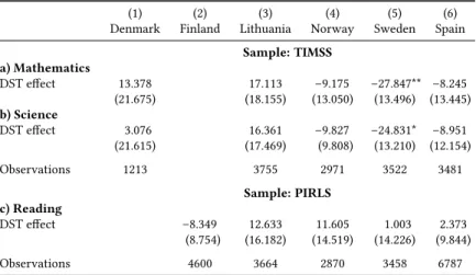
2.6 Country-specific impact of the clock change on students’ performance . . . 29
2.7 Impact of the clock change in the pooled sample, 2 weeks before and after . . . 31
2.8 Impact of the clock change by countries, 2 weeks before and after . . . 32
2.9 Fourth graders’ performance by gender and age . . . 34
2.10 Impact of the clock change on eighth-graders, 1 week before and after . . . 36
A2.1 Descriptive statistics (PIRLS) . . . 41
A2.2 Differences in covariates before and after the treatment (PIRLS) . . . 42
A2.3 Impact of the clock change on performance in math (pooled sample) . . . 43
A2.4 Impact of the clock change on performance in science (pooled sample) . . . 44
A2.5 Impact of the clock change on performance in reading (pooled sample) . . . 45
A2.6 Students’ math performance by books at home . . . 46
A2.7 Students’ science performance by books at home . . . 47
A2.8 Students’ reading performance by books at home . . . 48
xiii
test language is spoken at home . . . 50 A2.11 Students’ reading performance by gender and by whether
test language is spoken at home . . . 51 A2.12 Country-specific impact of the clock change on perfor-
mance in math . . . 52 A2.12 Continued . . . 53 A2.13 Country-specific impact of the clock change on perfor-
mance in science . . . 54 A2.13 Continued . . . 55 A2.14 Country-specific impact of the clock change on perfor-
mance in reading . . . 56 A2.14 Continued . . . 57 A2.15 Impact of the clock change on performance in math (pooled
sample, two weeks before and after) . . . 58 A2.15 Continued . . . 59 A2.16 Impact of the clock change on performance in science (pooled
sample, two weeks before and after) . . . 60 A2.16 Continued . . . 61 A2.17 Impact of the clock change on performance in reading
(pooled sample, two weeks before and after) . . . 62 A2.17 Continued . . . 63 A2.18 Country-specific impact of the clock change on perfor-
mance in math (two weeks before and after) . . . 64 A2.18 Continued . . . 65 A2.19 Country-specific impact of the clock change on perfor-
mance in science (two weeks before and after) . . . 66 A2.19 Continued . . . 67 A2.20 Country-specific impact of the clock change on perfor-
mance in reading (two weeks before and after) . . . 68 A2.20 Continued . . . 69 3.1 Descriptive statistics by whether students take up BAföG
or not . . . 94 3.2 Different specifications for the predicted probability not to
take up BAföG, i.e., Pr (NTU = 1|X) . . . 100
3.2 Continued . . . 101
3.3 Predicted probabilities for non-take-up of BAföG by differ-
ent levels of the students’ impulsivity and impatience . . . 104
3.4 Duration of receipt and non-take-up probability Pr (NTU = 1|X) . . . 107
3.5 Predicted probabilities for non-take-up of BAföG by the students’ East German background and whether parents received other social transfers last year . . . 108
3.6 Parents’ financial support does not impact on non-take-up 109 3.7 Missing data does not impact on non-take-up (full sample) 111 3.8 Simulation quality does not impact on non-take-up (sample after 2006) . . . 112
A3.9 Exemplary BAföG calculation . . . 116
A3.10 Basic allowances of incomes and assets between 2002 and 2015 . . . 118
A3.11 Level of needs 2002–2015 . . . 120
A3.12 Sensitivity of NTU and beta error . . . 125
A3.13 Robustness of East German background effect . . . 127
4.1 Pre-treatment descriptive statistics . . . 146
4.1 Continued . . . 147
4.2 Determinants of the application for a merit scholarship: Logit model . . . 149
4.3 Knowledge level of non-applicants at baseline (wave 1) . . 151
4.4 Ordered logit model for scholarship knowledge: average semi-elasticities . . . 154
4.5 ITT effects on knowledge: Ordered logit model . . . 156
4.6 ITT effects for full sample and heterogeneous effects: OLS 158 4.7 ITT effects on pre-application outcomes: OLS . . . 160
4.8 ITT effects of application for a BFW-scholarship, approxi- mation of the relevant sample: OLS . . . 162
4.9 Success probabilities for applications at baseline: OLS . . . 164
4.10 ITT effects of application for a BFW-scholarship, by gender: OLS . . . 165
A4.11 Influence of similarity on applications in the role model treatment group . . . 172
A4.12 Influence of similarity on applications in the role model treatment group by number of similarities . . . 173
A4.13 Influence of self-assessed fit on applications in the role model treatment group . . . 175
A4.14 Pre-treatment reasons for not applying . . . 180
with political association . . . 182 A4.16 Continued . . . 183 A4.17 Application requirements of the German Begabtenförderungswerke
with other association . . . 184
AME Average marginal effects
BA Bachelor’s degree
BAföG Federal Education and Training Assistance Act BFW Begabtenförderungswerke
DST Daylight saving time
FAFSA Free Application for Federal Student Aid GDR German Democratic Republic
GPA Grade point average HLM Hierarchical linear model
IEA International Association for the Evaluation of Educational Achievement
ITT Intent-to-treat IV Instrumental variable
MA Master’s degree
NTU Non-take-up rate
OLS Ordinary least squares
PIRLS Progress in International Reading Literacy Study SAT Scholastic Aptitude Test
xvii
STEM Science, technology, engineering, and mathematics
TIMSS Trends in International Mathematics and Science Study
TSLS Two-stage least-squares
Introduction
The first studies in the economics of education were concerned with recogniz- ing human capital as an investment good (Schultz, 1959, 1961; Becker, 1993) and to overcome the fact that “our knowledge about national wealth is almost wholly restricted to the non-human components, that is, to reproducible physical capital and land” (Schultz, 1959, p. 110). Nowadays, investments in education are seen as “one of the top priority policy areas of governments around the world [...] [and] an essential element in global economic compe- tition” (Hanushek, 2009, p. 39). Accordingly, there is large interest by both policy makers and researchers with respect to the determinants of educa- tional achievements, the outcomes of education, and the lessons to be learned from and for educational policies.
Generally, educational policy aims at both remedying market imperfec- tions and establishing equality of opportunity. Market imperfections with respect to education are mainly produced by the fact that education exerts pos- itive externalities, resulting in individual human capital investments below the social optimum. Moreover, imperfect information about costs and benefits of education provides another rationale for intervention—both for efficiency and equity reasons. Apart from that, equity considerations themselves give rise to public involvement in the provision and financing of education. There- fore, the common ground is typically to secure equality of opportunity, so that all people have equal opportunities to access education—irrespective of their socio-economic background.
This dissertation consists of two separate parts. The first part seizes on the determinants of educational achievement, whereas the second part is
1
model the determinants of educational achievement in an education produc- tion function where student and family characteristics, but also institutional and school factors, influence test scores. Institutional factors comprise the form of funding, the autonomy of schools, and age of tracking, while school- related factors include class size, instruction time, and teacher quality.
Among the school-related factors—and probably even among all topics ever studied in the economics of education—, class size has received most attention by scholars and policy makers. Research of the past decades has shown that class size reductions are a very costly, though relatively ineffective, means to improve students’ performance (see Hanushek (1999) or Hanushek (2006) for a review of the literature).
A school-level factor that has received far less scientific attention is school starting time. Though parents, teachers, and the media favor later school starting times with well rested students, the question whether ringing the school bell later increases students’ school performance is still unresolved. On the one hand, circadian rhythms are tied to the light-dark cycle and getting up early in the dark might be related to shorter bed hours. Many studies suggest, indeed, a positive correlation between hours slept and grades in middle and high school (Wolfson and Carskadon, 2003; Shochat et al., 2014).
Yet, on the other hand, recent evidence on whether later school start times cause increased achievements yields mixed results (Edwards, 2012; Carrell et al., 2011; Hinrichs, 2011; Heissel and Norris, 2015).
Johanna Sophie Quis, Guido Heineck, and I take a broader perspective to investigate the relationship between sleep and students’ performance in Chapter 2 of this dissertation: We provide first evidence on whether the spring transition from standard to daylight saving time (DST) induces short- run consequences on elementary school students’ test performance. Based on the public discussion and the pertinent literature from medicine, psychology, and biology, we hypothesize that elementary school children might suffer from sleep deprivation in the week after the clocks were advanced by one hour.
We exploit the fact that six European states collected data on more than
22,000 students in the Trends in International Mathematics and Science Study
(TIMSS) and the Progress in International Reading Literacy Study (PIRLS)
during the transition to DST in spring 2011. In a regression discontinuity
design, we compare the performance of students randomly allocated to testing
dates in the week before the clock advance with those allocated to testing dates in the week after the clock advance.
Our estimates for the DST-effect are very small in magnitude and not statistically significantly different from zero. Therefore, our results challenge the prevailing public opinion that daylight saving time should be abandoned because of its detrimental effects on school children’s performance.
The second part of this dissertation shifts the focus to equality of oppor- tunity in higher education and students’ reaction to offers of different forms of student financial aid.
Student financial aid aims at overcoming credit constraints resulting from capital market imperfections: Human capital theory (Becker, 1993) argues that human capital cannot serve as a collateral for a loan as “Free men are not for sale” (Schultz, 1959, p. 111) and lenders cannot force graduates to deploy their full potential productively to prevent moral hazard. Therefore, access to higher education will depend on parents’ assets if students are credit constrained and student financial aid is unavailable. Although most industrialized countries provide student financial aid to secure equality of opportunity, the intergenerational persistence in educational attainment is still high (Hertz et al., 2008; Heineck and Riphahn, 2009; Riphahn and Schieferdecker, 2010; Blossfeld et al., 2016). The results of Cameron and Heckman (1998, 2001) and Carneiro and Heckman (2002) provide a potential explanation for this finding: The authors argue that only long-run factors such as the parents’ permanent income and endowment restrict the transition to higher education, and that short-run liquidity constraints are no relevant obstacle. According to them, intergenerational persistence of educational attainment is an artifact of a failure to account for the high unobserved ability or motivation of those students who make their way successfully through the educational system. Once these long-run constraints and dynamic sample selection are accounted for, they find no effect of parental income on US students’ access to higher education in the National Longitudinal Survey of Youth. They argue that mitigating short-run liquidity constraints cannot increase enrollment and graduation rates substantially.
The findings of Cameron and Heckman (1998, 2001) are, however, chal- lenged by several more recent studies: Belley and Lochner (2007), for example, use the same database but draw upon cohorts born 20 years later. While they can replicate Heckman and co-authors’ findings for the older cohorts, they find a large increase in the impact of family income on college enrollment for the younger cohort, even after long-run factors have been accounted for.
Furthermore, the impact of parents’ income on completion of at least 2 years
decker (2010) investigate the importance of parental background factors in the transition from high school to university in Germany. With data from the German Socio-Economic Panel Study (SOEP), they show that parental income remains a large and significant predictor of enrollment probabilities, even though long-run characteristics such as parental education and sample selection into the pool of high school graduates are accounted for.
With respect to future governmental intervention, it is important to understand why the inter-generational educational mobility to German uni- versities is relatively low (OECD, 2014, p. 93), although higher education institutions do not charge tuition, and student aid transfers based on the Federal Education and Training Assistance Act (BAföG) provide lucrative funding that should facilitate studying for students from low-income families.
Our analysis in chapter 3 is an attempt to offer new insights into this matter. Michael Kalinowski and I study whether low-income students eligible to receive BAföG do indeed claim their benefits or whether features in the design of the federal aid scheme prevent students from claiming their need- based student aid amounts.
We construct a microsimulation model for the SOEP 2002–2013 to estimate the respective aid amounts students would have received, had they filed an application for need-based aid. The results indicate that about two fifths of the eligible low-income students do not take up their entitlements.
In a second step, we consider several potential explanatory factors shed- ding light on the reasons for students’ non-take-up of BAföG. More specif- ically, we employ instrumental variable techniques and a sample selection model to investigate whether different utilities from claiming, information constraints, parents’ claiming of other welfare benefits, cultural differences, and time-inconsistent preferences can explain students’ behavior. We find that the expected duration of benefit receipt and students’ financial need are inversely related to non-take-up. Nevertheless, increasing benefits by 10%
decreases non-take-up by only 4.1% on average. In addition, students who
can draw upon past experience of older siblings in filing the complex applica-
tions for BAföG are considerably more likely to claim the benefits. Therefore,
these findings provide evidence that information asymmetries contribute to
explaining why student financial aid may not work as intended. Moreover,
we include a variable indicating whether parents lived in the former socialist
East Germany before reunification to proxy inherited preferences about the
welfare state. We find that significantly more students socialized in East Germany choose to take up student aid compared to similar West German students. Lastly, our results suggest that, although BAföG as a combination of grant and zero-interest loan is by construction rather profitable, it seems to favor debt aversion of highly impulsive and impatient students in line with the predictions from the “Economic Theory of Self-Control” (Thaler and Shefrin, 1981).
Although we abstain from claiming causality for the mechanisms we in- vestigate, our results provide indications that the German need-based student financial aid scheme may not be suited to provide equality of opportunity if non-claiming students have to spend a considerable time on working to earn their living. Students who have to work many hours and can devote less resources to studying are, consequently, more susceptible to prolong studying (Avdic and Gartell, 2015), perform worse academically (Stinebrick- ner and Stinebrickner, 2003; Callender, 2008), or drop out without a degree (Triventi, 2014). The students we are analyzing have already made their way to university. Nevertheless, dropping out is harmful to equality because of the non-trivial monetary returns accruing from completing higher education, the
“sheepskin effect” (Heckman et al., 2006, e.g.). It remains an open question to which extent the factors fostering higher education students’ decisions not to claim also carry over to high school graduates. It is, however, plausible to assume that high school students’ level of information about BAföG and their ability to cope with the complex paperwork is, if anything, lower than that of higher education students. The high complexity of BAföG and its design might, therefore, also dissuade a significant share of credit-constrained students from studying at all. Bettinger et al. (2012) substantiate this assump- tion for the US. They show that assisting low-income families in filling out student aid application forms increases aid take-up, college enrollment, and completion substantially.
While chapter 3 studies federal need-based aid, the subsequent chapter 4 is devoted to the analysis of federal merit-based aid. The main goal of merit- based scholarships is not to provide equal access for all students but rather to efficiently promote the most talented ones. This efficiency goal, currently budgeted with almost EUR 244 million of fiscal revenue in Germany, implies that the most talented students, irrespective of their social background, should receive a scholarship.
Yet, two thirds of all German merit-based aid holders come from fami-
lies where at least one parent achieved a college degree, though students of
academic background only make up half of the overall student population
(Middendorff et al., 2009, p. 24). The magnitude of this difference is sur-
that information asymmetries even plague students’ claiming of broad and therefore well-known need-based aid (see chapter 3 but also Dynarski and Scott-Clayton (2006); King (2006); Bettinger et al. (2012)) make it very likely that information asymmetries also play a role with respect to merit-based aid: Only 1% of all German higher education students receive a scholarship so that the mere existence of this funding possibility might be unknown to many students from families unacquainted with higher education. Moreover, while eligibility for need-based aid is unequivocally regulated by law, the eligibility criteria to successfully apply for merit-based aid are vague and vary between the privately-owned foundations distributing the federal funds to students. Insider information and encouragement from parents might thus be all the more helpful and necessary for students to consider applying. If information asymmetries kept eligible students off applying, scholarships would not meet the efficiency goal to further promote the talent of promising students.
Although only 1% of all German students are funded by merit-based schol- arships, investigating social selectivity in the German merit-based aid system is important: Besides the risk of talent loss, being funded by a scholarship in Germany opens up access to several other non-monetary privileges such as mentoring and support by influential previous scholarship holders, and serves as a strong signal in the curriculum vitae of those who succeeded in the highly competitive selection procedure. A social selective scholarship system based on a considerable amount of public funds raises thus also normative equality concerns.
Chapter 4 explores whether information asymmetries between students able to draw upon the guidance of at least one college-experienced par- ent (“academic students”) and those from families where no one studied (“non-academic students”) are one of the causes for different application probabilities.
There are two reasons for why I focus on students’ applications for
scholarships rather than on their successes. First, I want to assess which
share of the non-academic students’ under-representation in the scholarship
body is caused by their scant or distorted information about the scholarship
system. I cannot isolate this channel when investigating success probabilities
because many more factors influence the scholarship award. On the one
hand, for example, scholarship providers may (consciously or unconsciously)
discriminate against “educationally deprived” students. On the other hand,
these students’ performance in the assessment centers may be under threat if they feel stereotyped as a minority (Steele et al., 2002). Second, even if scholarship foundations are able to objectively select the best students, their choice is limited to the pool of applicants. Therefore, from a policy perspective, increasing the share of eligible applicants from non-academic homes provides the basis to secure an efficient allocation of funds.
A causal effect of information asymmetries could not be isolated even if data on students deciding for or against applying for a scholarship were available. Therefore, I conducted a web-based field experiment between the years 2013 and 2015, based on a sample of more than 5,000 German higher education students. I randomly assigned students either to the control group or one of two treatment groups. The first treatment group read a general primer about scholarships, based on the scholarship information publicly available. In the second treatment group, participants additionally read an interview with a real, current scholarship holder. He or she provided tailored information on the detailed application process and probabilities of success.
To ease identification, the scholarship holder resembled the participant in several characteristics, acting as a role model.
At baseline, the results indicate indeed that non-academic students apply
less often than students from academic homes, keeping a range of eligibility
characteristics constant. Of the non-applicants at baseline, non-academic
students are moreover significantly worse informed, suggesting that the de-
cision to abstain from applying might not be well-grounded. Accordingly,
both treatments increase the knowledge of non-academic students about
scholarships significantly. Yet, only the role model treatment increases non-
academic students’ application probabilities for federally funded merit-based
scholarships significantly. Information asymmetries are therefore one factor
why non-academic students are underrepresented in the German scholar-
ship system. Moreover, the public information about scholarships currently
provided online is not sufficient to compensate for the existent knowledge
differentials by parental background. Interpreting the role model treatment
as a simulation of the custom-fit insider information many academic students
can access through their parents, the decisive information is a glance behind
the scenes and the assurance that a similar person made it. As a consequence,
establishing mentoring programs at schools is a promising and inexpensive
endeavor to increase both efficiency and equality of opportunity in the merit
aid system.
Does the Transition into
Daylight Saving Time Affect Students’ Performance?
Stefanie P. Herber, Johanna Sophie Quis, and Guido Heineck
2.1 Introduction
80 countries around the world
1are currently exposed to a shift in sleep patterns twice a year when they switch between daylight saving time (DST) and standard time (ST): In the northern hemisphere, clocks are set forward by one hour in spring to DST and set backward by one hour in fall to ST. While the phase delay in fall rewards us with an additional hour of sleep, the phase advance in spring implies that we have to get up one hour earlier—while the sunlight lags one hour behind.
Ever since its first introduction, the change to DST has been critically discussed. Germany and Austria-Hungary introduced DST in 1916
2in order to save energy and to better match sleep-wake cycles with daylight times.
Various recent studies challenge that DST saves energy (e.g., Kellogg and Wolff, 2008; Aries and Newsham, 2008; Kotchen and Grant, 2011; Sexton and Beatty, 2014). Another strand of research discusses whether the shift to DST increases traffic and work-related accidents (e.g., Hicks et al., 1983; Barnes and Wagner, 2009) or not (e.g., Ferguson et al., 1995; Lahti et al., 2011), influences stock market returns (e.g., Kamstra et al., 2000) or not (e.g., Gregory-Allen
1 Data compiled from the CIA World Factbook Central Intelligence Agency (2013).
2 Reichsgesetzblatt (RGBI) 1916. Bekanntmachung über die Vorverlegung der Stunden während der Zeit vom 1. Mai bis 30. September 1916, RGBl 1916, p. 243.
9
2014), to name just some.
So far, no clear conclusions can be drawn as to whether DST is indeed harmful enough to affect outcomes measurably and whether its potential costs outweigh its supposed benefits. Most previous studies suffer from small sample sizes (as already noted by Gregory-Allen et al., 2010) or fail to control for unobserved structural differences before and after the time change or between DST- and non-DST-countries. Nevertheless, a recent representa- tive survey puts the share of DST-opponents in the German population at nearly three quarters (forsa Gesellschaft für Sozialforschung und statistische Analysen mbH, 2015) and there, as well as in many other countries, regular petitions urge parliaments to break with the tradition of changing clocks twice a year.
In addition, and although one can set one’s clocks to reading regularly in the newspapers that DST should be abandoned because it is detrimental to school children’s performance (e.g., Schmidt, 28.03.2009; Draper, 05.03.2015), there is hardly any scientific evidence on whether the time change affects school performance. To the best of our knowledge, there is only one study (Gaski and Sagarin, 2011) on the long-run impact of the semiannual clock changes and students’ performance in the Scholastic Aptitude Test (SAT) in Indiana, USA. The authors report SAT scores in DST-adopting counties to be lower by 16 points (which equals 16% of a standard deviation). Yet, we doubt that the difference the authors find can be explained by the clock change as Gaski and Sagarin (2011) do not account for potential structural differences between counties that might drive the results. Moreover, most US states experience changes of more than 10 points in mean SAT scores in reading and math over time (National Center for Education Statistics, 2013), half of the SAT-taking schools experience a rise or fall in scores by 10 points every year, and about 20% tend to have 20 points higher or lower test scores when compared to the previous year (College Board, 2014).
This chapter is the first to study whether the clock advance induces short-run consequences on students’ performance in six European states.
We exploit the fact that several countries collected data for the international
student assessments Trends in International Mathematics and Science Study
(TIMSS) and Progress in International Reading Literacy Study (PIRLS) during
the transition from ST to DST in spring 2011. This approach provides us
with a sample of more than 22,000 students. Hypothesizing that elementary
school children might suffer from sleep deprivation and a relatively “earlier”
school start in the week after the switch to DST, we mimic the underlying basic structure of a regression discontinuity design by investigating whether moving the clock forward by one hour affects students’ performance.
This mechanism is backed up by a rich literature on the relationship between sleep and performance, which indicates that cumulative or complete sleep deprivation decreases cognitive test performance (e.g., Astill et al., 2012; Van Dongen et al., 2003; Banks and Dinges, 2007; Goel et al., 2009).
Whether the rather mild and short-term disturbances of the circadian system introduced by the clock change are large enough to affect children’s school performance significantly is, however, unknown. If so, this would not only make a case for another debate on whether to abandon DST or not, but would also call into question the validity of exams and international student achievement tests timed around the clock change. If the shift into DST does not cause large enough drops in students’ performance, this would cast doubt on the trustworthiness of the claim that children suffer measurably from the clock change.
Our results challenge the predominant expectation that the clock change introduces strong and measurable changes in children’s school performance.
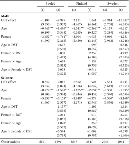
Although we do find small decreases in performance after the clock change in most countries for math and science, these effects are very small in magnitude and not significantly different from zero at neither point of the performance distribution. Moreover, the treatment effects for reading are pointing to the opposite direction and are of similar magnitude, though also not statistically significant. Our results are moreover robust to varying the time window around the clock change and cannot be explained by the young age of the fourth-graders in our main sample.
2.2 Effects of the clock advance
2.2.1 The circadian clock
In each of us ticks a circadian clock that determines when we sleep and when we wake. Daylight serves as a zeitgeber to our inner clock and synchronizes our sleep-wake patterns approximately (circa) to the daily (dian) rotation of the Earth. Our organism is tied to that inasmuch as the hormone melatonin regulates our sleep-wake-cycle by sending us to sleep. When it gets dark, our bodies produce melatonin and we begin to feel sleepy. At dawn, the production is stunted and we awake.
In Europe, this bio-chemical system is disturbed each spring when the
clock is set forward by one hour in the very early morning hours of the last
melatonin levels are still up and we feel sleepy. In the evenings, we have difficulty falling asleep. This deprivation of sleep persists until the DST and the light-dark cycle are synchronized, or in other words, until we have settled the dispute between the alarm and inner clock (Valdez et al., 2003, p. 146).
2.2.2 Sleep, light, and cognitive performance
Both sleep and light are also correlated with cognitive performance. Light does not only affect vision but exerts a direct positive effect on the functioning of the brain and its availability increases cognitive performance (Heschong et al., 2002; Vandewalle et al., 2006, 2009).
The positive association between sleep duration and cognitive test per- formance of adults is well documented (e.g., Van Dongen et al., 2003; Banks and Dinges, 2007; Goel et al., 2009).
3A recent meta-analysis shows that also for 5-12 years aged children, sufficient sleep is significantly related to higher cognitive performance, less internalizing (e.g., anxiety, sadness) and exter- nalizing (e.g., aggression, hyperactive behavior) behavioral problems, and, especially, better performance in school (Astill et al., 2012, and references therein). At the same time, children’s attention, memory, and intelligence seem to be unaffected by sleep duration (Astill et al., 2012).
Correlational studies draw the picture of a positive relationship between self-reported hours of sleep and grades in middle and high school (consult Wolfson and Carskadon (2003) or Shochat et al. (2014) for a review). Children seem to be sensitive to small or modest changes in sleep duration. In that vein, Vriend et al. (2013) show that reducing habitual sleep duration of 32 children by one hour for four consecutive nights affected children’s mood and emotional regulation negatively and decreased their cognitive performance.
2.2.3 Sleep and performance after the clock change
It is not clear, in how far all these processes carry over to the clock change, especially with respect to elementary school children who are the subject of this study.
3 The performance enhancing effects of sleep even seem to pay off in monetary terms.
Instrumenting sleep duration with the local sunset time, Gibson and Shrader (2014) estimate the causal effect of hours slept on wages. Speculating that an earlier sunset drives people to bed earlier, the authors provide evidence that sleeping one hour more each night increases wages by 16%.
First, there is mixed evidence on how long the sleep-wake cycle needs to adapt after the clock change. Results from both early and recent studies indicate that children and adolescents lose between 40 and 50 minutes of sleep following the switch from ST to DST (Reese, 1932; Barnes and Wagner, 2009). Schneider and Randler (2009) report that school children showed a higher daytime sleepiness after the time change. The adaption process to the new regime can take up to several weeks, depending on chronotype and sleep patterns during weekends (Valdez et al., 2003; Schneider and Randler, 2009). In contrast, adjustments to phase delays as encountered when clocks are reset to ST, traveling westwards, or moving from daytime shift work to night shift work are easier and faster (Hauty and Adams, 1965a,b; Lemmer et al., 2002; Niu et al., 2011).
Second, the impact of a single small short-term shift in the circadian clock is only rarely studied and if so with small sample sizes and in an artificial setting. For instance, Burgess et al. (2013) simulate small disturbances of the circadian clock in 11 adults, who reacted with significantly slower reaction times in a Psychomotor Vigilance Test. Monk and Aplin (1980) analyze the performance of 39 adults during the shift from DST to ST, i.e., during the phase delay in fall. After waking under the standard clock time, subjects showed enhanced performance in calculation tests. Yet, the authors cannot separate this effect from the simultaneous effect of a better mood on awakening.
A separate strand of the literature analyzes how delaying school starting times affects educational achievements. Although these studies are rather focused on medium-term outcomes than on the effects of short-term distur- bances of the circadian clock, we want to briefly review this literature as delaying school start by one hour mimics the reverse of the shift into DST at least temporarily.
Recently, three economic studies provided quasi-experimental evidence of a later school start time on students’ achievements. Although these studies can rely on larger samples and exogenous variation instead of self-reported measures from survey data, the results are, again, mixed.
Edwards (2012) exploits the fact that US middle schools start the school day at different times to reduce the costs of the public transportation system.
Using between and within variation, he finds a 2-3 percentage point increase in standardized math and reading test scores when school starts one hour later.
Carrell et al. (2011) show that delaying course start times by 50 minutes
increased students’ achievements at a US-military post-secondary institution
by as much as a one standard deviation increase in teacher quality. The
authors use variation from two sources: First, starting times were shifted
allocated to later courses could not use the additional time in the mornings to sleep longer because they were required to attend the early breakfast with their fellow students. Carrell et al. (2011) argue that late-starting students could have taken a nap between breakfast and their first class, thereby getting more sleep and performing better throughout the day. Given that the military institution prohibited napping (p. 78), it is contradictory that additional sleep should be the main driver of higher performance. To us, it seems equally likely that students in late courses achieved higher grades because the empty time-slot allowed them to repeat and, thereby, better remember the course content. This could also explain why the treatment estimates of attending an early class lose their statistical significance once student fixed effects are included.
In contrast to Carrell et al. (2011), Hinrichs (2011) uses longitudinal indi- vidual data on the US high school achievement test ACT and exploits, in his main analysis, exogenous variation from a policy change in the US: While Minneapolis and some of its surrounding districts shifted school starting hours backwards, its Twin City St. Paul and surroundings retained the old starting times. The author does not find evidence for the hypothesis that ringing the school bell later increased students’ performance.
Heissel and Norris (2015) take a different approach to investigate the effect of school starting times on students’ performance. They exploit the differences in the availability of sunlight before school between time zones both in an instrumental variable approach and a geographic regression dis- continuity design. Within-comparisons of students who move across the time zones in Florida show that starting schools one hour later increases test scores up to 0.1 standard deviation for pubescent adolescents, whereas the effects are smaller and insignificant for prepubescent children. Their estimates from the regression discontinuity design in Tennessee generally support these findings.
To the best of our knowledge, there is only one study on the relationship between DST and performance of students. Using the variation in DST- regimes between counties of the US State of Indiana, Gaski and Sagarin (2011) identify the long-run effects of DST on county-wide SAT test performance.
The authors find test results to be significantly worse in counties that advance
and set back their clocks each year when compared to counties sticking to
ST permanently.
Note that our approach, outlined in the following section, is different.
Gaski and Sagarin (2011) compare long-run average performance in counties that do or do not change their clocks and interpret their results as persistent difference in performance. Their approach comes at the risk of mistakenly interpreting structural differences between counties as causal effects. The authors do, for instance, not control for the proximity to large cities outside Indiana. It seems plausible that the counties close to Chicago, Cincinnati, or Louisville change the clocks to synchronize working times for commuters from Indiana. Worse SAT scores could then, e.g., be due to the reduced time commuting parents and their children spend at home together or a less privileged background. The latter would also explain why the families cannot afford living closer to the city. In contrast to that, our study focuses on short- run effects of the clock change within DST-adapting countries. Exploiting the random allocation of schools to test dates before and after the clock change as a natural experiment allows us to separate the effect of the transition into DST from structural or institutional differences. If the mild disturbance of the inner clock affects sleep patterns so much that performance in the week after the change suffers, we should be able to observe a short-run dip in performance.
2.3 Method
We analyze the shift to DST as a natural experiment to study before-after differences in students’ performance. As sleep-wake cycles and human per- formance are thought to synchronize within about one week after the clock change (Valdez et al., 2003), we restrict the sample to schools tested within one week before and one week after the change to DST.
4More specifically, we regress the test score TS
ijcof student i in school j and country c on the treatment indicator, DST
ijc, a set of controls, x
ijc, and the constant η
0. α
0is the coefficient of interest as it captures the effect of the switch to DST on student test scores. We run hierarchical linear models (HLM) with maximum likelihood to account for the nested structure of the data.
5The error term is, therefore, a composite taking care of the different
4 As we show in the robustness checks, our results are not sensitive to the time restriction.
5 We also estimated ordinary least squares (OLS)-models with standard errors clustered on the highest level, i.e., on the school level in the country-specific regressions or the country level in the pooled sample. The coefficients estimated with OLS were similar. Moreover, all our results are very similar in a typical regression discontinuity design where the running variable is equal to the number of days away from DST.
TS
ijc= η
0+ α
0· DST
ijc+ x
ijc· β + υ
j+ ν
c+ ϵ
ijc. (2.1) As students are only tested once—either before or after the clock change—
our research design relies on the identification assumption that the assign- ment to test dates before (control group) and after (treatment group) the shift to DST was random. The TIMSS and PIRLS testing dates are restricted to a given time span determined by the end-dates of the school year. Within this time window, school coordinators and testing agencies agree on a spe- cific date. Given sufficient capacity on the test agency’s side, the students’
performance is assessed on that day.
6The sampling is, therefore, unrelated to regional characteristics (south/west, rural/urban) that might have also driven the test score results.
7This procedure might, however, open up the possibility of self-selection into treatment and control group. For example, if coordinators of good schools preferred test dates before the shift to DST because they anticipate a dip in their students’ performance, we may mistak- enly contribute a negative treatment effect to the clock change, while it only captures a generally worse performance of students tested later.
Although we cannot fully rule out that consideration of the clock change mattered when school coordinators proposed a testing date, we consider it unlikely that coordinators were aware of the clock change and its potential harmful effect on their students’ performance as dates were scheduled well in advance.
8Moreover, assessments took place towards the end of the respective school terms, i.e., during a period where schools schedule examination board meetings, field days, or other activities filling the students’ and teachers’
timetables. Therefore, we expect that it is challenging enough to arrange a test date that fits the students’, teachers’, and testing agencies’ schedule without consideration of the clock change. Apart from that, it is impossible to identify single schools in the data later, reducing any possible incentive
6 Most schools were tested only on one day per study. In 3.57% of TIMSS- and 3.35% of PIRLS-schools, a few students were tested after the clock change, although their school was sampled before the clock change—probably because they were ill during the main testing time and data for the missing students was collected later.
7 A systematic geographical sampling would have introduced the risk of mistaking structural differences or differences in the availability of daylight between eastern and western areas within a country for a performance difference with respect to the DST-shift.
8 According to the National Research Coordinators of the five TIMSS countries in our sample, the majority of schools was first contacted some 6 to 8 months prior to the testing day.
for school coordinators to optimize their students’ performance with respect to test time selection, given that they were indeed aware of the clock change date.
We check the plausibility of the identifying assumption by comparing treatment and control group students on variables that might drive test performance. To do this, we test whether covariate means differ statistically significantly between treatment and control group. To account for the fact that very small differences between treatment and control group lead to high values for the t-statistic if the sample size is large, we also calculate the scale-free normalized differences as suggested by Imbens and Wooldridge (2009, p. 24). More specifically, we take the differences in means between covariates before, x
before, and after, x
after, the treatment and normalize them by their sample standard deviations, using the respective sample variances before, s
2before, and after, s
2af ter, the treatment:
∆
x= x
after− x
beforeq
s
2before+ s
2after. (2.2)
Following the authors’ rule of thumb, we interpret differences larger than a quarter of a standard deviation as indication of selection bias and sensitivity of linear regression with respect to model specification.
To account for potential differences in performance over the week, e.g., a
“blue Monday effect” or exhaustion over the week (Laird, 1925; Guérin et al., 1993), but also to investigate whether the DST-effect fades out over the week, we include control variables for each testing day of the week, day , and its interaction with the treatment indicator:
9TS
ijc=η
1+ α
1· DST
ijc+
5
X
d=2
γ
d· day
id+
5
X
d=2
δ
d· day
id· DST
ijc+ x
′ijc· β + υ
j+ ν
c+ ϵ
ijc.
(2.3) We use Monday as the reference category. Therefore, α
1represents the treatment effect for Mondays after the treatment. The marginal effect of the time change on the Tuesday under DST equals then, for instance, the
9 Please note that we thereby allow the treatment effect to vary non-linearly over days of the week. We also investigated whether imposing a more restrictive functional form, such as quadratic or cubic time trends, change our results. As we did not find evidence of increased fit and our results remained similar, we decided in favor of the specification presented here.
2.4 Data
The International Association for the Evaluation of Educational Achievement (IEA) has been assessing fourth- and eighth-graders’ reproduction, applica- tion, and problem solving skills in several areas of math and science since 1995 in the Trends in International Mathematics and Science Study (TIMSS).
Moreover, the IEA measures trends in fourth-graders’ reading literacy and comprehension every five years in the Progress in International Reading Liter- acy Study (PIRLS).
We can make use of several fortunate coincidences in the latest currently available waves of 2011 which we use for the following analyses: First, 2011 is the only year for which we can use assessment data for all three testing areas (math, science, and reading) because both TIMSS and PIRLS data were collected. Secondly, while data on the exact date of the testing was not contained in previous waves, this information is available in the 2011 waves. Lastly, as student achievement data were collected in the last months of the respective countries’ school terms, the field phases of several countries coincided with the transition into DST. In TIMSS 2011, there was an overlap between fourth-graders’ testing dates and the clock change in seven countries. Being especially interested in performance differences on the Monday after the clock change (which was March 28, 2011), we have to exclude the two countries that lack test data on Mondays (Finland and Ireland).
After excluding four students who were tested on a Sunday and 309 cases with missings on our covariates, our analytic sample from TIMSS contains 8,813 fourth-graders in 364 schools from Denmark, Lithuania, Norway, Spain, and Sweden.
10As Denmark did not participate in PIRLS 2011, our PIRLS sample includes Lithuania, Norway, Sweden, and Spain, but also Finland where students’ reading performance was assessed on all weekdays. After listwise deletion of 357 cases with missing values, our analytic PIRLS sample sums up to 13,255 fourth-grade students clustered in 508 schools.
TIMSS and PIRLS follow a matrix-sampling approach, meaning that there are many more questions asked in total than answered by a single student in the assessment booklets. Whereas students answer only one booklet, each
10 We focus on students in grade 4 as the data for eighth-graders do only include two countries (Sweden and Finland) for the respective time period and reading literacy is not assessed in grade 8. We do, however, draw on the eighth-graders sample in our robustness checks.
item is contained in more than one booklet. The IEA uses this overlap to construct an estimate of the achievements in the student population with the help of scaling methods from item-response theory (see Mullis et al. (2009a, p. 123), Mullis et al. (2009b); Yamamoto and Kulick (2012)). To account for the uncertainty introduced by imputing the scores, the IEA provides five plausible values of the achievement scores. We retain this uncertainty by using all five plausible values in the following analyses.
11Achievement scales range usually from 300 to 700 points. To establish comparability over time and between countries, the IEA scaled achievement test scores in 1995 (TIMSS) and 2001 (PIRLS) to an international mean of 500 and a standard deviation of 100.
Note that we focus on TIMSS for the following short description of our data in order to save space. We provide statistics for our PIRLS sample in the appendix (tables A2.1 and A2.2) and outline only main points in this section.
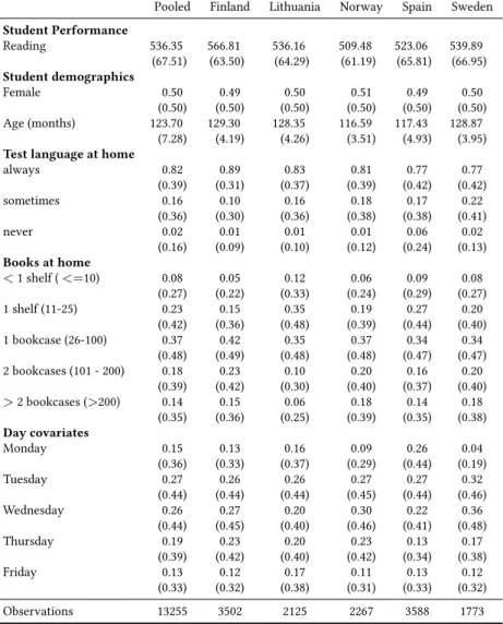
Table 2.1 gives an overview of the plausible values for the countries in our sample, showing that students perform between the intermediate and the high international benchmark, which are set at 475 and 550 points. On average, students achieve scores of about 509 points in math (S.D. ≈ 72) and 515 points in science (S.D. ≈ 70). Spanish students score lowest and Danish as well as Lithuanian students highest in math. In the science assessment, test scores are highest for Swedish and lowest for Norwegian children. For PIRLS, we find an average of 536 points in reading (S.D. ≈ 68), and that the best readers in our sample are the Finnish students, while the elementary school children in Norway achieve the lowest scores (cf. appendix table A2.1).
Table 2.1 contains further descriptive statistics on our later controls. We include gender and age in months to investigate heterogeneous effects and to account for potential differences between treated and controls. All of our students are in grade 4 and the average student is about 10 years old. Half of the sample is female. The high performing Danish, Finnish, Swedish, and Lithuanian students are, on average, one year older than the lower performing Norwegian and Spanish children.
11 More specifically, we apply Rubin’s Rules (Rubin, 1987) to combine adjusted coefficients and standard errors from all plausible values as implemented in the multiple imputation (mi) commands in Stata.
Student Performance
Math 509.14 537.29 537.47 496.54 490.41 505.95
(71.97) (68.66) (71.57) (68.81) (69.15) (67.50)
Science 515.47 528.38 518.35 496.23 515.67 534.84
(69.90) (71.01) (65.32) (64.13) (70.93) (74.84) Student demographics
Female 0.50 0.54 0.49 0.51 0.49 0.48
(0.50) (0.50) (0.50) (0.50) (0.50) (0.50)
Age (months) 122.70 130.55 128.30 116.59 117.40 128.76
(7.28) (4.59) (4.28) (3.48) (5.00) (3.93) Test language spoken at home
always 0.79 0.83 0.83 0.80 0.74 0.78
(0.41) (0.37) (0.37) (0.40) (0.44) (0.41)
sometimes 0.18 0.16 0.16 0.18 0.19 0.21
(0.39) (0.37) (0.36) (0.39) (0.39) (0.41)
never 0.03 0.01 0.01 0.01 0.07 0.01
(0.16) (0.08) (0.10) (0.12) (0.26) (0.11) Books at home
<1 shelf (<=10) 0.09 0.09 0.13 0.06 0.09 0.06
(0.28) (0.28) (0.33) (0.24) (0.29) (0.24)
1 shelf (11-25) 0.25 0.27 0.36 0.19 0.26 0.20
(0.44) (0.45) (0.48) (0.39) (0.44) (0.40)
1 bookcase (26-100) 0.35 0.37 0.35 0.36 0.34 0.34
(0.48) (0.48) (0.48) (0.48) (0.47) (0.47)
2 bookcases (101 - 200) 0.17 0.16 0.10 0.20 0.16 0.22
(0.37) (0.37) (0.30) (0.40) (0.36) (0.41)
>2 bookcases (>200) 0.14 0.11 0.07 0.19 0.15 0.18
(0.35) (0.31) (0.25) (0.39) (0.36) (0.38) Day covariates
Monday 0.14 0.14 0.10 0.14 0.17 0.15
(0.35) (0.35) (0.30) (0.35) (0.37) (0.36)
Tuesday 0.27 0.17 0.24 0.22 0.35 0.29
(0.44) (0.38) (0.43) (0.42) (0.48) (0.46)
Wednesday 0.30 0.48 0.29 0.34 0.24 0.28
(0.46) (0.50) (0.45) (0.47) (0.43) (0.45)
Thursday 0.20 0.17 0.21 0.23 0.20 0.18
(0.40) (0.37) (0.41) (0.42) (0.40) (0.39)
Friday 0.09 0.04 0.16 0.07 0.05 0.09
(0.28) (0.19) (0.37) (0.25) (0.21) (0.28)
Observations 8813 564 2116 2328 2208 1597
Notes: Own calculations for the pooled sample based on TIMSS 2011. Mean values and standard deviations (in parentheses) of the pooled and country-specific samples. The day covariates indicate the percentage of students tested on that day. We used all five plau- sible values and applied Rubin’s rule (Rubin, 1987) to calculate the appropriate standard deviations of the average student performances.
We include an indicator for whether students wrote the test in the lan- guage they speak at home to control for language-related differences in test scores. About 80% do indeed always stick to the test language at home and only 2-3% indicate to never use it at home. To control for the children’s socio- economic background by proxy, we add the number of books at home.
12Most children indicate that their parents have 26-100 books (one bookcase) at home. In 14% of the cases, children report more than two bookcases (more than 200 books) at home. The average number of books at home is relatively high in Sweden, Norway, and Finland, though relatively low in Lithuania.
When turning to test days, the table shows that most students were tested on Tuesdays or Wednesdays. In our TIMSS-sample, 14% of the overall sample was tested on Mondays (table 2.1), thereof 43% before and 57% after the switch to DST. 15% of the PIRLS-students were tested on a Monday (appendix table A2.1), 28% of them under ST and 72% under DST.
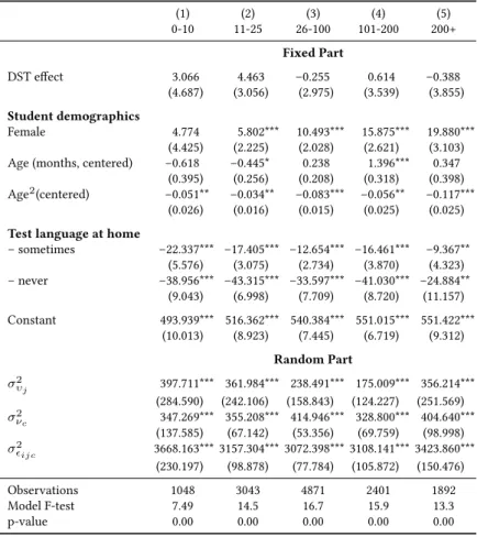
As outlined in the previous section, we test for (normalized) differences between students treated before and after the clock change. The results are reported in table 2.2 for TIMSS and appendix table A2.2 for PIRLS. While absolute differences are statistically significantly different from zero for most variables, they show neither a systematic pattern nor are the normalized dif- ferences above the critical value of 0.25 suggested by Imbens and Wooldridge (2009, p. 24). Including these covariates in the following regressions controls for slight differences between groups that should not substantially affect our results.
1312 There are three main reasons why we favor this often used proxy for the educational, social, and economic background of the family. First, the number of books at home is easily comparable across countries (Wößmann, 2004). Second, the predictive power of the books variable with respect to student performance is higher than that of parents’ educational background (Wößmann, 2003). Third, while books at home are reported for nearly all students, parents’ educational achievement is systematically missing for about one third of the cases in our TIMSS sample and about 12% in our PIRLS sample. Missing cases are a selective sample of students with a low number of books at home.
13 We also investigate differences in other proxies for the students’ socio-economic status between “treated” and “untreated” students, e.g., own possessions including books, study desks, or computers. We do not find a systematic pattern within and over countries that would point to a selection of specific students or schools to the treatment or control group.
Moreover, our results are very similar after including these variables as additional controls.
Table 2.2: Differ ences in co variates befor e and after the tr eatment (TIMSS)
BeforeAfterBefore-AfterNormalizeddifference Mean(S.D.)Mean(S.D.)Diff.(P-value) Studentdemographics Female0.50(0.50)0.50(0.50)0.00(0.93)–.001 Age(months)123.51(7.11)122.03(7.36)1.48(0.00)–.144 Testlanguageathome –always0.77(0.42)0.81(0.39)–0.04(0.00)0.076 –sometimes0.21(0.41)0.16(0.37)0.05(0.00)–.090 –never0.02(0.15)0.03(0.17)–0.01(0.11)0.024 Booksathome: –lessthanoneshelf(<=10)0.08(0.27)0.09(0.29)–0.01(0.03)0.032 –oneshelf(11-25)0.24(0.43)0.27(0.44)–0.02(0.01)0.038 –onebookcase(26-100)0.34(0.48)0.36(0.48)–0.01(0.19)0.020 –twobookcases(101-200)0.17(0.38)0.16(0.37)0.02(0.06)–.029 –morethantwobookcases(>200)0.16(0.37)0.13(0.33)0.03(0.00)–.069 Dayoftest: –Monday0.13(0.34)0.15(0.35)–0.01(0.05)0.029 –Tuesday0.20(0.40)0.32(0.47)–0.12(0.00)0.195 –Wednesday0.37(0.48)0.24(0.43)0.13(0.00)–.203 –Thursday0.19(0.39)0.21(0.41)–0.02(0.00)0.044 –Friday0.10(0.30)0.07(0.26)0.03(0.00)–.071 Observations400048138813 Notes:Thetablereportsthemeanvaluesandstandarddeviationsofallcovariatesforthecontrolgroup(testedbeforethe transitionintoDST)andthetreatmentgroup(testedafterthetransition).Thethirdcolumncontainsthedifference meansandtherespectivep-valuesfromtestingthehypothesisthatthetwomeansareequal.Thelastcolumnreportsthe normalizeddifferencesassuggestedbyImbensandWooldridge(2009,p.24).CalculationsbasedonTIMSS2011.2.5 Results
2.5.1 Performance-effects of the clock change in the pooled sample
Table 2.3 reports the effects of the clock change on students’ performance in math, science, and reading for the pooled sample of all countries. Note that the students tested in math were also tested in science and vice versa, because both fields were part of the TIMSS study. Most of the TIMSS students did also participate in the PIRLS reading assessment, but not all of them.
14Table 2.3: Impact of the clock change on students’ perfor- mance (pooled sample)
(1) (2) (3) (4)
Sample: TIMSS (8,813 observations) a) Mathematics
DST effect –4.042 –9.131 –3.462 –8.139
(3.512) (8.742) (3.074) (7.663) b) Science
DST effect –3.892 –10.601 –3.433 –9.439
(3.444) (8.586) (2.909) (7.293) Sample: PIRLS (13,255 observations) c) Reading
DST effect 0.506 8.180 0.309 4.072
(2.695) (6.626) (2.306) (5.686)
Sociodemographic controls X X
Days & interactions X X
Notes: Own calculations for the pooled sample based on TIMSS and PIRLS 2011. Sociodemographic controls: gender (reference: male), age (centered), age (centered, squared), books at home (refer- ence: one bookcase), test language spoken at home (reference: al- ways); day and interaction controls: weekday (reference: Monday), weekday×DST. Standard errors in parentheses. *p <0.1, **p <
0.05, ***p <0.01.
In the HLM specification without covariates (table 2.3, column 1), students scored about 4 points lower in both math and science when tested during
14 We would have liked to also present within-analyses for students who participated in both TIMSS and PIRLS and completed one study before and the other one after the clock change.
Unfortunately, TIMSS and PIRLS were always conducted at consecutive days within the same week. Nevertheless, we verified that the results presented here are not sensitive to the order in which the tests took place.