Nonlinear Cointegration Analysis and the Environmental Kuznets Curve

IHS Economics Series Working Paper 224

July 2008

Nonlinear Cointegration Analysis and the Environmental Kuznets Curve

Seung Hyun Hong

Martin Wagner

Impressum Author(s):

Seung Hyun Hong, Martin Wagner Title:

Nonlinear Cointegration Analysis and the Environmental Kuznets Curve ISSN: Unspecified

2008 Institut für Höhere Studien - Institute for Advanced Studies (IHS) Josefstädter Straße 39, A-1080 Wien

E-Mail: o ce@ihs.ac.atffi Web: ww w .ihs.ac. a t

All IHS Working Papers are available online: http://irihs. ihs. ac.at/view/ihs_series/

This paper is available for download without charge at:

https://irihs.ihs.ac.at/id/eprint/1846/

Nonlinear Cointegration Analysis and the Environmental Kuznets Curve

Seung Hyun Hong, Martin Wagner

224

Reihe Ökonomie

Economics Series

224 Reihe Ökonomie Economics Series

Nonlinear Cointegration Analysis and the Environmental Kuznets Curve

Seung Hyun Hong, Martin Wagner July 2008

Institut für Höhere Studien (IHS), Wien

Institute for Advanced Studies, Vienna

Contact:

Seung Hyun Hong Department of Economics Concordia University

1455 de Maisonneuve Blvd. West Montreal, Quebec H3G 1M8 email: shhong@alcor.concordia.ca

Martin Wagner

Department of Economics and Finance Institute for Advanced Studies Stumpgergasse 56

1060 Vienna, Austria : +43/1/599 91-150

email: Martin.Wagner@ihs.ac.at

Founded in 1963 by two prominent Austrians living in exile – the sociologist Paul F. Lazarsfeld and the economist Oskar Morgenstern – with the financial support from the Ford Foundation, the Austrian Federal Ministry of Education and the City of Vienna, the Institute for Advanced Studies (IHS) is the first institution for postgraduate education and research in economics and the social sciences in Austria.

The Economics Series presents research done at the Department of Economics and Finance and aims to share “work in progress” in a timely way before formal publication. As usual, authors bear full responsibility for the content of their contributions.

Das Institut für Höhere Studien (IHS) wurde im Jahr 1963 von zwei prominenten Exilösterreichern – dem Soziologen Paul F. Lazarsfeld und dem Ökonomen Oskar Morgenstern – mit Hilfe der Ford- Stiftung, des Österreichischen Bundesministeriums für Unterricht und der Stadt Wien gegründet und ist somit die erste nachuniversitäre Lehr- und Forschungsstätte für die Sozial- und Wirtschafts- wissenschaften in Österreich. Die Reihe Ökonomie bietet Einblick in die Forschungsarbeit der Abteilung für Ökonomie und Finanzwirtschaft und verfolgt das Ziel, abteilungsinterne Diskussionsbeiträge einer breiteren fachinternen Öffentlichkeit zugänglich zu machen. Die inhaltliche Verantwortung für die veröffentlichten Beiträge liegt bei den Autoren und Autorinnen.

Abstract

Recent years have seen a growing literature on the environmental Kuznets curve (EKC) that resorts in a large part to cointegration techniques. The EKC literature has failed to acknowledge that such regressions involve unit root nonstationary regressors and their integer powers (e.g. GDP and GDP squared), which behave differently from linear cointegrating regressions. Here we provide the necessary tools for EKC analysis by deriving estimation and testing theory for cointegrating equations including stationary regressors, deterministic regressors, unit root nonstationary regressors and their integer powers. We consider fully modified OLS estimation, specification tests based on augmented and auxiliary regressions, as well as a sub-sample KPSS type cointegration test. We present simulation results illustrating the performance of the estimators and tests. In the empirical application for CO

and SO

emissions for 19 early industrialized countries over the period 1870-2000 we find evidence for an EKC in roughly half of the countries.

Keywords

Integrated Process, Nonlinear Transformation, Fully Modified Estimation, Nonlinear Cointegration Analysis, Environmental Kuznets Curve

JEL Classification

C12, C13, Q20

Contents

1 Introduction 1

2 Econometric Theory 3

2.1 Setup and Assumptions ... 3

2.2 OLS Estimation... 7

2.3 Fully Modified OLS Estimation... 8

2.4 Specification Testing based on Augmented and Auxiliary Regressions... 10

2.5 KPSS Type Tests for Cointegration... 14

3 Simulation Performance 18

3.2 Performance of the Augmented and Auxiliary Regression Tests ... 19

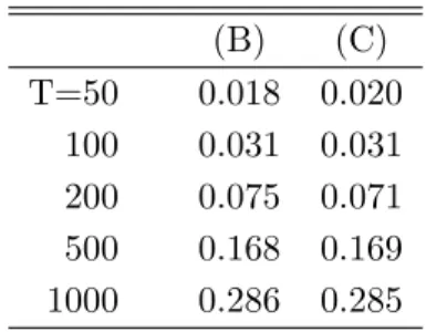
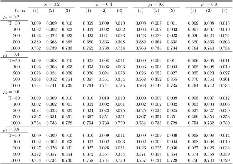
3.3 Performance of the KPSS Type Tests... 25

4 Environmental Kuznets Curves 26 5 Summary and Conclusions 36

References 38

Appendix A: Proofs 42

Appendix B: Additional Material for the Empirical Study 49

1 Introduction

Since the seminal work of Grossmann and Krueger (1993, 1995) many econometric studies of the relationship between measures of economic development (typically proxied by per capita GDP) and pollution, respectively emissions, have been conducted. Survey articles like Stern (2004) or Yandle, Bjattarai, and Vijayaraghavan (2004) count more than one-hundred refereed publications. Most of the papers focus on a specific conjecture, the so called ‘environmental Kuznets curve’ (EKC) hypothesis, which postulates an inverted U-shaped relationship between the level of economic de- velopment and the degree of income inequality. The term EKC refers by analogy to the inverted U-shaped relationship between the level of economic development and the degree of income in- equality postulated by Kuznets (1955) in his 1954 presidential address to the American Economic Association.

The largest part of the empirical EKC literature estimates parametric EKCs, however, also other estimation strategies have been followed in the empirical EKC literature: non-parametric EKCs (see e.g. Millimet, List, and Stengos, 2003), semi-parametric EKCs (see e.g. Bertinelli and Strobl, 2005) or EKCs using spline interpolations (see e.g. Schmalensee, Stoker, and Judson, 1998). Within the parametric EKC literature many studies rely upon unit root and cointegration analysis given the widespread non-rejection of the unit root hypothesis for GDP. With the exception of very few papers who note and bypass in one way or another the associated problems (see Bradford, Fender, Shore, and Wagner, 2005; M¨ uller-F¨ urstenberger and Wagner, 2007; Wagner, 2008), the empirical EKC literature fails to acknowledge the implications of the presence of nonlinear transformations of unit root processes. In a typical EKC, compare (19) below, emissions are regressed on GDP and GDP squared. Since (log per capita) GDP is often well characterized as being a unit root process, GDP squared is a nonlinear transformation of an integrated process and regressions involving such processes require different asymptotic theory than the usual ‘linear’ unit root and cointegration analysis.

In this paper we derive the asymptotic distributions of both the OLS estimator as well as of a

fully modified OLS (FM-OLS) estimator of equations containing deterministic variables, stationary

regressors, integrated regressors and integer powers of integrated regressors. The results we obtain

resemble in several respects that of linear cointegration analysis as derived in Phillips and Hansen

(1990) and rely upon the important contributions of Chang, Park, and Phillips (2001) and Park

and Phillips (1999, 2001). First, the OLS estimator is consistent, but its limiting distribution is

contaminated by so called second order bias terms, rendering valid inference infeasible. Second, the proposed FM-OLS estimator has a limiting distribution that is free of second order biases and thus forms the basis for asymptotically valid χ

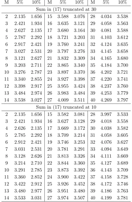
-inference for certain hypotheses. Third, this property of the limiting distribution of the FM-OLS estimator also forms the basis for specification testing based on augmented respectively auxiliary regressions including higher order polynomial powers of the integrated regressors and/or polynomial powers of additional integrated regressors. In this re- spect we consider tests based on both the Wald and Lagrange Multiplier testing principles. Fourth, we consider a KPSS type (compare Kwiatkowski, Phillips, Schmidt, and Shin, 1992) cointegration test to directly test the null hypothesis of nonlinear cointegration for a given specification. Since the asymptotic distribution of this test is contaminated by nuisance parameters we follow Choi and Saikkonen (2005) and present a sub-sample version of the test that has an asymptotic distribution free of nuisance parameters. Since the sub-sample test can be used in conjunction with the Bonfer- roni bound we investigate the potential performance gains that can be realized by using adjusted Bonferroni bound test procedures that are less conservative, such as those proposed in Simes (1986) or Rom (1990).

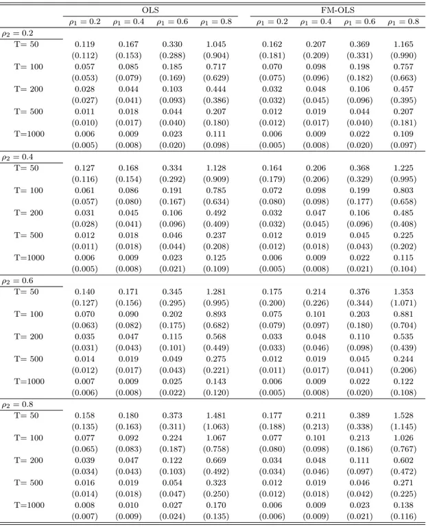
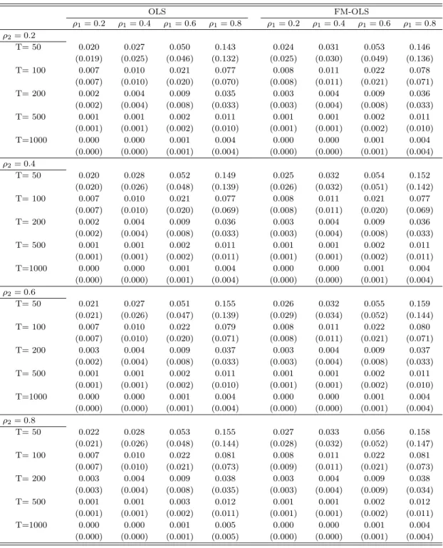
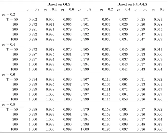
We conduct a small simulation study to assess the performance of the proposed methods. The findings show that the FM-OLS correction has only modest effects on the biases of the coefficients estimated by FM-OLS compared to the – also consistent – OLS estimates. The effects are much larger on the tests, whose performance hinges crucially on applying appropriate FM-OLS correc- tions. The Wald and Lagrange Multiplier tests behave very similarly and perform very well in terms of size. Their power performance depends, as expected, quite strongly upon the auxiliary regressors as well as the alternative considered. With respect to the sub-sample KPSS type tests we note that all considered modifications of the Bonferroni bound lead to very similar performance in the simulations. The KPSS type tests tend to be undersized for small samples and their power increases quite slowly with the sample size. However, their power is quite similar for all considered alternatives, which is consistent with the fact that the KPSS type tests are not specified against any particular alternative.

After the simulations we turn to the empirical analysis where we study the relationship between

CO

respectively SO

emissions and GDP for a panel of 19 early developed countries over the

period 1870–2000. When considering a quadratic formulation of the EKC we find support, based

on the LM specification test, for eight countries for CO

emissions and for five countries SO

emissions. Allowing for smooth asymmetries by modeling a cubic EKC leads to non-rejections of a

nonlinear cointegrating relationship in three more countries for both CO

and SO

emissions. The turning points implied by the FM-OLS coefficient estimates are with very few exceptions reasonable in-sample values.

The paper is organized as follows. In Section 2 we derive the asymptotic results for the estimators and tests. Section 3 contains a small simulation study to assess the finite sample performance of the proposed methods and Section 4 contains the results of the EKC analysis. Section 5 briefly summarizes and concludes. Two appendices follow the main text: Appendix A contains the proofs of all propositions results and Appendix B collects additional material related to the empirical EKC analysis.

We use the following notation: As usual, the symbols ⇒ and →

signify weak convergence and convergence in probability, respectively. Definitional equality is signified by :=. Further, a

= O(T

) (respectively a

= O

(T

)) denotes that {a

} is at most of order T

(in probability).

Standard Brownian motions are denoted as W (r) or in short W , whereas Brownian motions with non-identity covariance matrices (specified in the context) are denoted with B(r) or B. For integrals of the form R

0

B(s)ds and R

0

B (s)dB(s) we use short-hand notation R

B and R

BdB. For notational simplicity we also often drop function arguments. With bxc we denote the integer part of x ∈ R and diag(·) denotes a diagonal matrix with the entries specified throughout. E denotes the expected value and L denotes the backward-shift operator, i.e. L{x

}

= {x

}

.

2 Econometric Theory

2.1 Setup and Assumptions

We consider the following equation including stationary regressors w

, i = 1, . . . , n, a constant, polynomial time trends up to power q and integer powers of integrated regressors x

, j = 1, . . . , m up to degrees p

y

= w

θ

+ D

θ

+ X

j=1

X

θ

+ u

, for t = 1, . . . , T (1) with w

:= [w

, . . . , w

]

, D

:= [1, t, t

, . . . , t

]

, x

:= [x

, . . . , x

]

, X

:= [x

, x

, . . . , x

]

and the parameter vectors θ

∈ R

, θ

∈ R

and θ

∈ R

. Furthermore define for later use X

:= [X

, . . . , X

]

, Z

:= [w

, D

, X

]

and p := P

j=1

p

.

In a more compact way,

y = wθ

+ Dθ

+ Xθ

+ u (2)

= Zθ + u,

with y := [y

, . . . , y

]

, u := [u

, . . . , u

]

, Z := [w D X] and θ = [θ

θ

θ

]

∈ R

and

w :=



  w

.. . w



  ∈ R

, D :=



  D

.. . D



  ∈ R

, X :=



  X

.. . X



  ∈ R

.

Let us next state the assumptions concerning the regressors and the error processes:

Assumption 1 The processes {∆x

}

, {w

}

and {u

}

are generated as

∆x

= v

= C

(L)ε

= X

j=0

c

ε

w

= C

(L)η

= X

j=0

c

η

u

= C

(L)ζ

= X

j=0

c

ζ

,

with the summability conditions C

(1) 6= 0,

X

j=0

j||c

|| < ∞ , X

j=0

j

||c

|| < ∞ , X

j=0

j

|c

| < ∞.

Furthermore we assume that the regressors are predetermined, i.e. we assume that the process {ξ

}

= {[ε

, η

, ζ

]

}

is a stationary and ergodic martingale difference sequence with na- tural filtration F

= σ ³©

ξ

ª

−∞

´

and denote the (conditional) covariance matrix by

Σ

=





Σ

Σ

Σ

Σ

Σ

Σ

Σ

Σ

σ



 := E(ξ

(ξ

)

|F

).

We also assume that Σ

:= Ew

w

> 0.

The above assumptions allow to draw on the asymptotic results of Chang, Park, and Phillips

(2001) and Park and Phillips (1999, 2001). The assumption that the regressors are predetermined

implies that the conditional expectation E(y

|F

) = 0, which is usual in nonlinear regression

theory. Considering the stationary regressors to have zero mean is only done for convenience and

is not a restriction since typically an intercept will be included in a regression. The assumption C

(1) 6= 0 implies that x

is indeed an integrated process whereas Σ

> 0 is mainly put in place for convenience as it is likely to be fulfilled in all practical applications.

Further additionally required moment assumptions given below are also similar to those formu- lated in Chang, Park, and Phillips (2001).

Assumption 2 For the process {ξ

}

the following conditions hold:

1. sup

E(kξ

k

|F

) < ∞ a.s. for some r > 4.

2. E

³

(ξ

)

ξ

´

= 0 for all i, j and for all l ≥ 1.

3. ζ

is i.i.d. with E(|ζ|

) < ∞ for some r > 8 and its distribution function is absolutely continuous with respect to the Lebesgue measure and for the characteristic function ϕ it holds that ϕ(λ) = o(|λ|

) as λ → ∞ for some δ > 0.

The above assumptions are sufficient for the following invariance principle to hold for {ξ

}

= {[v

, w

, u

]

}

using the Beveridge-Nelson decomposition (compare Phillips and Solo, 1992)

√ 1 T

[T r]

X

t=1

ξ

⇒ B(r) =



 B

(r) B

(r) B

(r)



 . (3)

Note here that it holds that B(r) = Ω

W (r) with the long-run covariance matrix Ω := P

h=−∞

E (ξ

ξ

).

We also define the one-sided long-run covariance Λ := P

h=0

E (ξ

ξ

) and both covariance matrices are partitioned according to the partitioning of ξ

, i.e.:

Ω =



 Ω

Ω

Ω

Ω

Ω

Ω

Ω

Ω

ω



 , Λ =



 Λ

Λ

Λ

Λ

Λ

Λ

Λ

Λ

λ



 .

When referring to quantities corresponding to only one of the nonstationary regressors and its powers, e.g. X

, we use the according notation, e.g. B

(r) or Λ

.

To study the asymptotic behavior of the estimators, we next introduce appropriate weighting

matrices, whose entries reflect the divergence rates of the corresponding variables. Thus, denote

with G(T ) = diag{G

(T ), G

(T ), G

(T )}, where for notational brevity we often use G := G(T ).

The three diagonal sub-matrices are given by:

G

(T ) :=



  T

. ..

T



  ∈ R

, G

(T ) :=



  T

. ..

T



  ∈ R

,

G

(T ) :=



  G

. ..

G



  ∈ R

with G

:=



  T

. ..

T



  ∈ R

.

Using these weighting matrices, we can define the following limits of the major building blocks. For t such that lim

t/T = r the following results hold:

T

lim

√ T G

(T )D

= lim

T→∞



  1

. ..

T



 



  1

.. . t



  =



  1

.. . r



  =: D(r)

T

lim

√ T G

(T )X

= lim

T→∞



  T

. ..

T



 



  x

.. . x



  =



  B

.. . B



  =: B

(r),

separating here the coordinates of v

= [v

, . . . , v

]

corresponding to the different variables x

. The first result is immediate and the second follows from Chang, Park, and Phillips (2001, Lemma 5). The stacked vector of the scaled polynomial transformations of the integrated processes is denoted as B

(r) := [B

(r)

, . . . , B

(r)

]

. We are confident that D as defined in (2) is not confused with D(r) defined above even when the latter is used in abbreviated form D in integrals.

Remark 1 More general deterministic components can be included with the necessary condition being that the correspondingly defined limit quantity satisfies R

DD

> 0, i.e. that the considered functions are linearly independent in L

[0, 1]. This allows in addition to the polynomial trends on which we focus in this paper e.g. also to include time dummies, broken trends or trigonometric functions of time (compare the discussion in Park, 1992).

The relationship postulated in (1) is restrictive in the sense that e.g. no cross-products of the

form x

x

or t

x

are included. Considering such cross-terms increases not only the flexibility of

the functional form but also immediately allows for an interpretation of the estimated relationship

as a Taylor expansion of an unknown nonlinear function. The theory developed in this paper,

based on the underlying results of Park and Phillips (1999, 2001), can be extended to include

these cross-terms. However, the curse of dimensionality will often limit the practical usefulness of

specifications including all cross-terms. Also for the empirical application in this paper we consider only one integrated regressor, namely per capita GDP.

2.2 OLS Estimation

We first study the asymptotic behavior of the OLS estimator. As in the linear cointegration case, its limiting distribution is contaminated by nuisance parameters due to serial correlation in the error process {u

}

and endogeneity of {∆X

}

. Both of these aspects are very similar to those in the linear case as in Phillips and Hansen (1990) and are summarized in Proposition 1.

Proposition 1 Let y

be generated from (1) with the regressors Z

and errors u

satisfying As- sumptions 1 and 2. Then the asymptotic distribution of the OLS estimator θ ˆ := (Z

Z )

Z

y is given by

G

(ˆ θ − θ) =





G

(ˆ θ

− θ

) G

(ˆ θ

− θ

) G

(ˆ θ

− θ

)





⇒



 



Σ

N

hR D ˜ D ˜

i

nR

DdB ˜

− R

DB

£R

B

B

¤

M

o hR B ˜

B ˜

i

nR B ˜

dB

− R B ˜

dB

Ω

Ω

+ M o



 

 (4)

where B

(r) := B

(r) − Ω

Ω

B

(r) with corresponding variance ω

:= ω

− Ω

Ω

Ω

and N

:= lim

T

P

t=1

w

u

. The random variable N

is normally distributed with mean Σ

:= E(w

u

) and variance depending upon the coefficients c

, c

, Σ

and σ

given in As- sumption 1. Furthermore

D ˜ := D − Z

DB

µZ

B

B

¶

B

, B ˜

:= B

−

Z B

D

µZ DD

¶

D,

and

M :=



  M

.. . M



  where M

:= Λ



 

 

1 2 R

B

(r)dr .. . p

R

B

(r)

dr



 

  . (5)

The limiting distribution of the consistent OLS estimator displayed in (4) is contaminated by so-

called second order bias terms: the serial correlation bias and the endogeneity bias, using the same

names in our nonlinear setup as used in the limiting distribution of the OLS estimator in the linear cointegration case (see Phillips and Hansen, 1990). Note that when X

is strictly exogenous, these bias terms vanish with Λ

= Ω

= 0. If this is not the case, standard inference on the parameters becomes invalid due to the presence of these bias terms.

Remark 2 Note that the serial correlation bias term M, which is due to correlation between u

and v

, appears not only in the limiting distribution of θ ˆ

, but also in that of θ ˆ

, reflecting the asymptotic correlation between deterministic and stochastic trends. Thus, putting these two blocks of the coefficient vector θ together in θ

:= £

θ

θ

¤

, we can explicitly identify the source of the serial correlation bias by writing the limiting distribution of the OLS estimator of θ

as

G

³ θ ˆ

− θ

´

⇒ µZ

JJ

¶

½Z

JdBu +

µ 0

M

¶¾ , for J (r) := £

D(r)

B

(r)

¤

and G

:= diag (G

, G

).

2.3 Fully Modified OLS Estimation

Two ways to remove the bias terms present in the OLS limiting distributions have been proposed in the cointegration literature. These are fully modified OLS (FM-OLS) estimation (see Phillips and Hansen, 1990) based on a direct non-parametric correction and dynamic OLS (D-OLS) esti- mation (see Saikkonen, 1991) where the correction is achieved by running lead and lag augmented regressions. In this paper we consider FM-OLS estimation which requires consistent estimators of the bias terms. In this respect define

M

:=



  M

.. . M



  , M

:= ˆ Λ



 

  T 2 P

x

.. . p

P

x



 

  , (6)

with a consistent estimator ˆ Λ

:= ˆ Λ

− Ω ˆ

Ω ˆ

Λ ˆ

. Once appropriately scaled the quantity M

in (6) converges to M as given in (5), which in conjunction with using the transformed dependent variable

y

:= y

− Ω ˆ

Ω ˆ

v

, y

:= [y

, . . . , y

]

leads to an asymptotic distribution that is free of bias terms as summarized in the following Proposition 2.

1For notational simplicity we ignore the dependence of y⁺ upon the specific consistent long-run covariance esti- mator chosen.

Proposition 2 Let y

be generated by (1) with the regressors Z

and errors u

satisfying Assump- tions 1 and 2. Define the FM-OLS estimator of θ as

θ ˆ

:= (Z

Z )

¡

Z

y

− A

¢ ,

with

A

:=



 Σ ˆ

0

M





with Σ ˆ

a consistent estimator of Σ

:= Σ

−Σ

Ω

Ω

and M

as given in (6) with consistent estimators of the required long-run (co)variances. Then the asymptotic distribution of θ ˆ

is given by

G

³ θ ˆ

− θ

´

=





G

(ˆ θ

− θ

) G

(ˆ θ

− θ

) G

(ˆ θ

− θ

)



 ⇒



 



Σ

N

hR D ˜ D ˜

i

R

DdB ˜

hR B ˜

B ˜

i

R B ˜

dB



 

 , (7)

with a normally distributed mean zero random variable N

:= lim

T

P

t=1

w

u

, where u

:= u

− Ω ˆ

Ω ˆ

v

.

Using the quantities defined in Remark 2 it holds more compactly written that G

³ θ ˆ

− θ

´

⇒

¡R JJ

¢

R

JdB

. The limiting distribution of G

(ˆ θ

− θ

) is free of second order bias terms and mixed normal with mean zero. This stems from the fact that the vector ˜ B

is, by construction, independent of B

.

As shown in Phillips and Hansen (1990, Theorem 5.1) the special form of the FM-OLS limiting distribution allows for asymptotic χ

-inference for testing certain linear hypothesis on the coef- ficients by using the Wald test. From the discussion in Phillips and Hansen (1990, p. 106), in particular from the corresponding proofs in their paper, it becomes clear that only certain linear hypotheses can be tested with asymptotic χ

-inference. A similar result that allows to test for certain hypotheses, which we formulate for notational convenience for θ

as defined in Remark 2, can be established in our setup.

Proposition 3 Let y

be generated by (1) with the regressors Z

and errors u

satisfying Assump- tions 1 and 2. Consider s linearly independent restrictions collected in

H

: Rθ

= r,

with R ∈ R

with full rank s and r ∈ R

. Furthermore let ω ˆ

denote a consistent estimator of ω

. Then it holds with Z

= [D X ] that the Wald statistic

W :=

³

R θ ˆ

− r

´

h ˆ ω

R ¡

Z

Z

¢

R

i

³

R θ ˆ

− r

´

(8) is under the null hypothesis asymptotically distributed as χ

under one of the following conditions:

(i) H

only involves coefficients with the same convergence rate, or

(ii) each of the restrictions in H

involves only one coefficient, i.e. the off-diagonal elements of R are all equal to 0.

The above result implies that for instance the appropriate t-statistic for coefficient θ

, with θ

a component of θ

, given by t

:=

ˆ

ωu.v(Z⁰Z)⁻¹_[i,i]

, is asymptotically standard normally distributed.

Note furthermore that hypothesis testing for the coefficients θ

can simply be based on their asymptotic normal distribution.

2.4 Specification Testing based on Augmented and Auxiliary Regressions Testing the correct specification of equation (1) is clearly an important issue. In this respect we are particularly interested in the prevalence of cointegration, i.e. stationarity of u

. Absence of cointegration can be due to several reasons. First, there is no cointegrating relationship of any functional form between y

and x

. Second, y

and x

are nonlinearly cointegrated but the functional relationship is different than postulated by equation (1). This case covers the possibilities of missing higher order polynomial terms or cointegration with a different functional form of the relationship.

Third, the absence of cointegration is due to missing explanatory variables in equation (1).

In a general formulation all the above possibilities can be cast into a testing problem within the augmented regression

y

= Z

θ + F (x

, q

, θ

) + φ

, (9) where F is such that F(x

, g

, 0) = 0 and q

denotes additional integrated regressors. If cointegration prevails in (1) then θ

= 0 and φ

= u

.

In many cases the researcher will not have a specific parametric formulation in mind for the

function F (·), which implies that typically the unknown F (·) is replaced by a partial sum ap-

proximation. This approach has a long tradition in specification testing in a stationary setup, see

Ramsey (1969), Phillips (1983), Lee, White, and Granger (1993) or de Benedictis and Giles (1998).

Given our FM-OLS results it appears convenient to replace the unknown F (·) by using polynomial powers of the integrated regressors, which will include higher order powers larger than p

for the components x

of x

and powers larger equal than 1 for the additional integrated regressors q

.

Of course this simple approach is also subject to the discussion in the introduction in that no multivariate expansion is considered. However, for specification analysis the advantage of a parsi- monious setup may outweigh the potential disadvantages of considering only univariate polynomials since a test based on such a formulation will also have power against alternatives where e.g. prod- ucts terms are present. Clearly, the power properties of tests based on univariate polynomials depend upon the unknown alternative F (·) and will be the more favorable the more F (·) ‘resem- bles’ univariate polynomials. This trade-off is exactly the same as in the stationary case, as also discussed in Hong and Phillips (2008).

Denote with ¯ X

:= [x

, x

, . . . , x

]

for j = 1, . . . , m, Q

:= [q

, q

, . . . , q

]

for i = 1, . . . , k, F

:= [ ¯ X

, . . . , X ¯

, Q

, . . . , Q

]

and F := [F

, . . . , F

]

. Using this notation the augmented polynomial regression including higher order polynomial powers of the regressors x

and polynomial powers of additional integrated regressors q

can be written as

y = Zθ + F θ

+ φ, (10)

with φ := [φ

, . . . , φ

]

. If equation (10) is well specified the parameters can be estimated consis- tently by FM-OLS according to Proposition 2 if the additional regressors q

fulfill the necessary assumptions stated in Section 2.1 which are now modified to accommodate additional regressors.

Assumption 3 When considering additional regressors q

and their polynomial powers define

˜

v

:= [v

, (v

)

]

= [∆x

, ∆q

]

, with v

= ∆q

and q

= [q

, . . . , q

]

. Assumptions 1 and 2 are extended such that they are fulfilled for the extended process v ˜

generated by C

(L)˜ ε

, with C

(L) and ε ˜

also extended accordingly.

Note that equation (10) can be well-specified for different reasons. The first is that (1) is a

cointegrating relationship, in which case consistently estimated coefficients ˆ θ

will converge to

their true value equal to 0. The second possibility is that (1) is misspecified, but the extended

equation (10) is well-specified. In this case at least some entries of ˆ θ

will converge to their non-

zero true values. In case that (10) and consequently also (1) are misspecified and φ

is not stationary,

spurious regression results similar to the linear case that lead to non-zero limit coefficients apply.

Consequently, a specification test based on H

: θ

= 0 is consistent against the three discussed forms of misspecification of (1) discussed in the beginning of the sub-section.

Testing the restriction θ

= 0 in (10) can be done in several ways. One is given by FM- OLS estimation of the augmented regression (10) and performing a Wald test on the estimated coefficients using Proposition 3. Another possibility is to use the FM-OLS residuals of the original equation (2) and to perform a Lagrange Multiplier RESET type test in an auxiliary regression.

These two possibilities are discussed in turn.

Proposition 4 Let y

be generated by (1) with the regressors Z

, Q

and errors u

satisfying Assumptions 1, 2 and 3. Denote with θ ˆ

the FM-OLS estimator of θ

in equation (10), with F ˜

= F − Z

(Z

Z

)

Z

F , and as above Z

= [D X] and let ω ˆ

be a consistent estimator of ω

. Then it holds that the Wald test statistic for the null hypothesis H

: θ

= 0 in equation (10), given by

T

:=

³ θ ˆ

´

³ F ˜

F ˜

´ θ ˆ

ˆ

ω

, (11)

is under the null hypothesis asymptotically distributed as χ

, with b := P

j=1

r

+ P

j=1

s

.

Note that the required variance and covariance estimates in Proposition 4 are all based on the (m + k)-dimensional process ˜ v

. The result given in Proposition 4 follows straightforwardly from Propositions 2 and 3.

The basis of the Lagrange Multiplier (LM) test are the FM-OLS residuals ˆ u

of (2), which are regressed on ˜ F in the auxiliary regression

ˆ

u

= ˜ F θ

+ ψ

. (12)

with ˆ u

= [ˆ u

, . . . , u ˆ

]

. Clearly, to allow for asymptotic standard inference the coefficients θ

have to be estimated by FM-OLS to achieve a second order bias free limiting distribution, since

the limiting distribution of the OLS estimator of θ

in (12) also depends upon second order bias

terms (see the proof of Proposition 5 in Appendix A for details). The FM-OLS estimator as well

as the test statistic for testing the hypothesis θ

= 0 are presented in the following proposition for

the case that (1) is well specified. Consistency of the tests against the above-discussed forms of

misspecification of (1) follows from the same arguments as for the Wald test.