Farm Wakes and their Impact on the Marine Boundary Layer
Inaugural-Dissertation
zur
Erlangung des Doktorgrades
der Mathematischen-Naturwissenschaftlichen Fakult¨ at
der Universit¨ at zu K¨ oln
vorgelegt von
Simon Karl Siedersleben aus M¨ unchen
Garmisch-Partenkirchen
2019
Berichterstatter, Gutachter:
Prof. Dr. Stefan Emeis Prof. Dr. Yaping Shao
Tag der m¨ undlichen Pr¨ ufung: 31.10.2019
ii
To my family
i
Abstract
Given the rising number of o↵shore wind farms, the e↵ect of wakes (the area downwind of wind farms characterized by a wind speed deficit) on downwind wind farms and their impact on the regional climate is discussed. This work investigates the spatial dimen- sions of wakes and the micrometeorological and regional climate impacts of o↵shore wind farms on the marine boundary layer based on mesoscale simulations using a wind farm parameterization (WFP) and airborne observations.
WFPs act as a momentum sink for the mean flow. However, WFPs di↵er on whether or not they add additional turbulent kinetic energy (TKE) to represent the enhanced mixing caused by wind farms. This thesis uses for the first time aircraft observations taken above and behind o↵shore wind farms to answer this uncertainty for stable conditions. The airborne measurements reveal that a TKE source and a horizontal resolution in the order of 5 km are necessary to represent the enhanced TKE (i.e. 20 times higher than in the ambient flow) above o↵shore wind farms.
Further, this thesis evaluates the simulated spatial extent of a wake by the use of airborne measurements taken on 10 September 2016. Observations and simulations show a wake longer than 45 km associated with a warming and drying at hub height in the order of 0.5 K and 0.5 g kg
1, respectively. Vertical cross-sections perpendicular to the wake reveal that warmer and dryer air was mixed towards the surface due to an inversion located within the rotor area. An analysis of 23 additional airborne measurements executed within the far-field of o↵shore wind farms suggests that an impact on the temperature is only visible in case of inversions in the vicinity of the rotor area and wind speeds over ⇡ 6 m s
1.
Based on the successful evaluations above and downwind of o↵shore wind farms, this thesis explores a future scenario including all o↵shore wind farms possibly installed at the German Bight to discuss potential impacts of large o↵shore wind farms on the regional climate by considering two case studies. The simulations suggest that the wakes of large o↵shore wind farms clusters are longer than 100 km associated with changes in the sensible and latent heat flux. The net impact on the MABL depends on the inversion height and the temperature gradient between sea surface temperature (SST) and air temperature. Therefore, the dominating impact of o↵shore wind farms can only be determined by simulations covering several years with the constraint that the inversion height is captured by the driving mesoscale model.
iii
Zusammenfassung
Durch die steigende Anzahl von O↵shore-Windparks werden die Auswirkungen von Nachl¨aufen großer O↵shore-Windparks auf leew¨arts gelegene Windparks diskutiert.
Zudem ist es unklar, inwiefern große O↵shore-Windparks die marine Grenzschicht und das regionale Klima beeinflussen k¨onnen. Diese Doktorarbeit untersucht die r¨aumliche Ausbreitung von Nachl¨aufen und deren Einfluss auf die Mikrometeorologie und das regionale Klima mit mesoskaligen Simulationen, die eine Windparkparametrisierung (WFP) verwenden. Die Simulationen werden mit Flugzeugmessungen evaluiert.
WFPs entziehen der Modellatmosph¨are kinetische Energie, der E↵ekt auf die tur- bulente kinetische Energie (TKE) wird jedoch unterschiedlich gehandhabt. Manche der WFPs repr¨asentieren eine zus¨atzliche TKE-Quelle im Modell, wohingegen andere nur eine Impulssenke darstellen. In dieser Arbeit werden erstmals beide Ans¨atze mit Flugzeugmessungen evaluiert, die ¨ uber und hinter großen O↵shore-Windparks durchgef¨ uhrt wurden. Hier hat sich gezeigt, dass eine TKE-Quelle und eine Aufl¨osung von 5 km oder feiner notwendig sind um die erh¨ohte TKE (20-mal h¨oher als in der unmittelbaren Umgebung) zu erfassen.
Basierend auf diesen Ergebnissen, evaluiert diese Arbeit die r¨aumliche Ausbreitung der Nachl¨aufe mit Flugzeugmessungen vom 10. September 2016. Beobachtung und Simulation zeigen erstmals einen Nachlauf mit einer L¨ange von ¨ uber 45 km, charakte- risiert durch eine Erw¨armung und trockenere Luft in Nabenh¨ohe in der Gr¨oßenordnung von 0.5 K und 0.5 g kg
1; 45 km leew¨arts des Windparks. Vertikale Schnitte senkrecht zur Windrichtung zeigen, dass aufgrund einer Inversion auf Nabenh¨ohe w¨armere und trockenere Luft nach unten gemischt wurde. Eine Analyse von 23 wei- teren beobachteten F¨allen zeigt, dass eine Temperatur¨anderung auf Nabenh¨ohe nur in Verbindung mit einer stabilen Schichtung und Windgeschwindigkeiten ¨ uber ⇡ 6 m s
1in H¨ohe des Rotorbereichs auftritt.
Basierend auf den erfolgreichen Evaluationen ¨ uber und leew¨arts großer O↵shore- Windparks, werden die Simulationen erweitert und ein Zukunftsszenario wird unter- sucht, das alle m¨oglichen o↵shore Windparks der Deutschen Bucht enth¨alt um erst- mals deren potentiellen Einfluss auf das regionale Klima zu diskutieren. Die Simu- lationen zeigen Nachl¨aufe von großen O↵shore-Windparkclustern mit einer L¨ange von
¨
uber 100 km in Verbindung mit ¨ Anderungen im sensiblen und latenten W¨armefluss w¨ahrend stabiler Bedingungen. Zudem ist der Temperaturgradient zwischen Meeres-
v
oberfl¨achentemperatur und Lufttemperatur entscheidend f¨ ur den Nettoeinfluss der
Windparks auf die marine Grenzschicht. Deswegen kann der dominierende Einfluss
auf das regionale Klima nur mit Simulationen bestimmt werden, die mehrere Jahre
abdecken und in der Lage sind die exakte H¨ohe der Inversionen ¨ uber der Deutschen
Bucht zu erfassen.
Contents
Abstract iii
Zusammenfassung v
Contents vii
1 General introduction and motivation 1
1.1 State of the art . . . . 1
1.1.1 Meteorological conditions at o↵shore sites . . . . 2
1.1.2 Wind speed deficit in the far-field of o↵shore wind farms . . . . 4
1.1.3 Micrometeorological, regional and global climate impacts of on- shore and o↵shore wind farms . . . . 7
1.2 Open questions and objectives of the present study . . . . 9
2 Dataset and method 12 2.1 Aircraft observations . . . . 12
2.1.1 Uncertainties in the aircraft measurements . . . . 12
2.1.2 Vertical profiles . . . . 12
2.1.3 In the far-field of o↵shore wind farms . . . . 14
2.1.4 Above o↵shore wind farms . . . . 14
2.2 Synthetic Aperture Radar Data (SAR) . . . . 16
2.3 Ground-based observations . . . . 17
2.4 Reanalysis Data: ECMWF analysis and ERA5 data . . . . 18
2.5 Wind farm parameterization . . . . 18
2.6 Numerical Setup . . . . 19
2.6.1 Control configuration . . . . 20
2.6.2 Sensitivity configurations . . . . 21
2.7 Wind farms implemented in the numerical model . . . . 22
2.8 Energy budget framework . . . . 23
3 Wind speed and TKE above o↵shore wind farms 25 3.1 Observations . . . . 25
3.1.1 Synoptics and mesoscale overview . . . . 25
vii
3.1.2 Wind speed above and next to the wind farms . . . . 26
3.1.3 TKE above and next to the wind farms . . . . 28
3.2 Control simulations . . . . 29
3.2.1 Evaluation of the background flow . . . . 29
3.2.2 Impact of wind farm parameterization on wind speed above wind farms . . . . 30
3.2.3 Impact of wind farm parameterization on TKE above wind farms 31 3.3 Sensitivity experiments . . . . 33
3.3.1 Sensitivity to horizontal and vertical resolution with an active TKE source . . . . 34
3.3.2 Sensitivity to vertical resolution with a disabled TKE source . . 36
3.3.3 Sensitivity to advection of TKE . . . . 36
3.3.4 Sensitivity to thrust coefficient . . . . 37
3.4 Discussion . . . . 38
3.5 Summary . . . . 40
4 The far-field of large o↵shore wind farms 43 4.1 Observation . . . . 43
4.1.1 Synoptic and mesoscale overview . . . . 43
4.1.2 Vertical structure of the atmosphere . . . . 44
4.2 Control run . . . . 46
4.2.1 Verification of the background flow . . . . 46
4.2.2 Evolution of the wind field upwind of the wind farms . . . . 47
4.2.3 Wake simulations . . . . 48
4.3 Sensitivity experiment . . . . 54
4.4 Discussion . . . . 56
4.4.1 Discussion of the wake simulations . . . . 56
4.4.2 Comparison to other cases . . . . 59
4.5 Summary . . . . 64
5 Potential micrometeorological and regional climate impacts of large o↵shore wind farms on the atmospheric boundary layer 66 5.1 O↵shore winds and stable conditions . . . . 66
5.2 Onshore winds and stable conditions . . . . 68
5.3 Discussion . . . . 71
5.4 Summary . . . . 73
6 Conclusion and outlook 75 6.1 Main results and conclusions . . . . 75
6.2 Suggestions for further studies . . . . 78
CONTENTS ix
Bibliography 81
Acknowledgments 93
Erkl¨ arung 95
1 General introduction and motivation
The first o↵shore wind farm was installed in 1991 at the coast of Vindeby, Denmark (Ørsted 2019). Associated with the nuclear catastrophe of Fukushima and the urgent need to stop climate warming, the wind energy o↵shore market has grown continuously since 1991. In 2017, Europe had a capacity of 16 GW installed o↵shore with 71 % in the North Sea (WindEurope 2017).
The wind speed downwind of large o↵shore wind farms can be reduced, even 50 km downwind, as indicated by satellite images (e.g., Christiansen and Hasager 2005; Hasager et al. 2005, 2015). O↵shore wind farms extract kinetic energy from the mean flow and convert it into electrical energy. Consequently, the wind speed is reduced downwind of large o↵shore wind farms. Throughout this thesis, we refer to this area, characterized by a wind deficit, as a wake. Given the rising number and the large size of o↵shore wind farms, two issues arise associated with wakes of o↵shore wind farms.
Wakes of upwind o↵shore wind farms reduce the energy harvesting in wind farms located downwind and, hence, the yields of stakeholders. O↵shore wind farms are clustered around transmission grids to redeem the high costs of installation and due to restrictions in space caused by military zones, pipelines and nature preserves. Hence, o↵shore wind farms are often only 10 km apart. Therefore, wind energy production losses are observed in downwind wind farms due to wakes from upwind wind farms (e.g., Nygaard 2014; Nygaard and Hansen 2016; Lundquist et al. 2018). Consequently, the wind energy industry has a great interest in determining the spatial scales of these wakes, especially under stable conditions when these wakes are expected to be longest due to the low turbulent vertical momentum transport (e.g., Emeis et al. 2016).
The impact of o↵shore wind farms on the regional climate is unclear. O↵shore wind farms represent an additional source of turbulence in the marine atmospheric boundary layer (MABL) (Fitch et al. 2012). Therefore, the temperature and moisture budget can be a↵ected by o↵shore wind farms and, hence, the turbulent fluxes between atmosphere and open ocean could be altered by wind farms. Consequently, the impact of large o↵shore wind farms on the MABL needs to be investigated.
These two topics are of major importance for stakeholders and a sustainable de- velopment of the o↵shore wind energy industry and are, hence, in the focus of ongoing research. The remaining chapter presents the state of the art in section 1.1, developing the research questions in section 1.2.
1.1 State of the art
To understand the nature of wakes of large o↵shore wind farms, knowledge about the MABL is necessary. This information is provided in section 1.1.1, followed by two sections, presenting previous findings about the length of wakes of large o↵shore
1
H ~5 H wave sub layer
constant flux layer Ekman sublayer free troposphere
flow
O(100) - O(1000) m
O(10) - O(100) m
Figure 1: The marine atmospheric boundary layer and its vertical structure. The blue line indicates the ocean’s surface with the wave height H. (Adapted from Emeis (2018). The wind turbine icon is taken from https://svg-clipart.com/white/Ta0k2H4-wind-turbine-clipart.)
wind farms (section 1.1.2) and observed and simulated impacts of wind farms on the micrometeorology and regional climate (section 1.1.3).
1.1.1 Meteorological conditions at o↵shore sites
O↵shore sites are characterized by higher wind speeds compared to onshore sites. The shape of vertical wind profiles is determined by the stability of the atmosphere and the surface roughness. The roughness of the ocean is linked to the wave height, and thus to the wind speed (Emeis 2018). Consequently, the surface roughness at o↵shore sites is controlled by the wind drag acting on the water surface. Charnock (1955) describes the surface roughness length over water as
z
0= ↵ u
2⇤g , (1)
with ↵, the Charnock parameter having a value of 0.011 for the open ocean according to Smith (1980) and u
⇤, the friction velocity. Following equation (1) with u
⇤= 0.33 m s
1, we can expect a surface roughness length over the ocean in the order of 10
4m that is at least two orders of magnitude lower than the surface roughness length for onshore sites (i.e. grassland has a surface roughness length of 0.01 m (Emeis 2018)). Consequently, the wind speed over the ocean is higher than at onshore sites. Additionally, the low surface roughness results in a vertical wind speed gradient with low shear at the rotor area, which in turn results in a balanced wind drag at the rotor tips. Such conditions are favorable for a slow fatigue of wind turbines.
The MABL is characterized by low turbulence in contrast to onshore sites. Two
1.1. STATE OF THE ART 3
ingredients are necessary for turbulence - shear and buoyancy. Given the low surface roughness of the ocean, shear is generally low over the ocean, resulting in low mechan- ical production of turbulence. Additionally, the surface temperature of the ocean is almost constant during the day due to the high heat capacity of water (Emeis 2018).
Consequently, large eddies as observed onshore can not exist o↵shore meaning that the turbulence generated by buoyancy is lower at o↵shore sites. Summarized, the turbu- lence o↵shore is lower than onshore (T¨ urk and Emeis 2010; Bodini et al. 2019).
The MABL is generally shallower than the boundary layer at onshore sides (Emeis 2018), rooted in the low turbulence at o↵shore sites. That is important to recognize when considering the dimensions of modern wind turbines. A hub height of ⇡ 100 m and rotor diameter of ⇡ 150 m are quite common, resulting in a rotor tip reaching a height of ⇡ 175 m. Consequently, wind farms are high enough to interact with the constant flux layer and the Ekman sublayer (Fig. 1). Within the constant flux layer, turbulent fluxes only vary with ± 10 %, reaching a height of ⇡ 10 % of the height of the MABL. Above the constant flux sublayer is the Ekman sublayer, characterized by a clockwise turning of the wind direction due to decreasing surface friction. At the top of the Ekman sublayer no friction is present anymore, hence, the wind is geostrophically balanced (Emeis 2018).
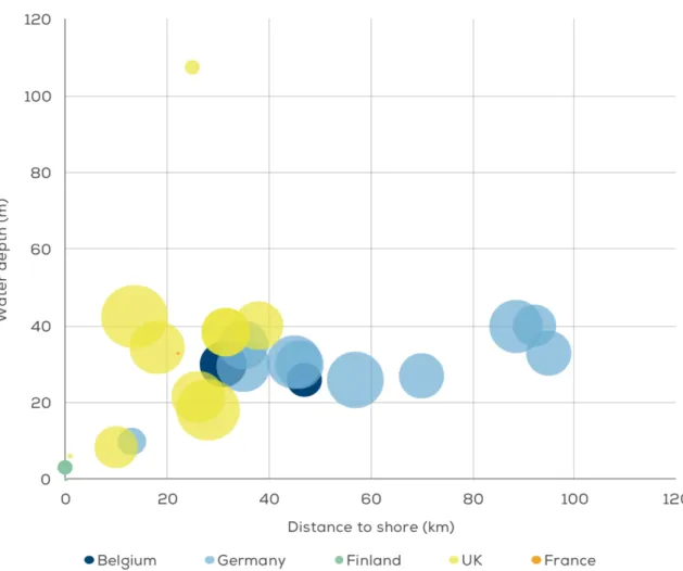
Most o↵shore wind farms in the North Sea that were under construction in 2017, are located at sites not further than 60 km away from the coast (Fig. 2) (WindEurope 2017), having the advantage that the installation of wind turbine platforms is easier in these regions due to water depths less than 60 m (Fig. 2). Additionally, the costs for transmission grids and maintenance can be minimized.
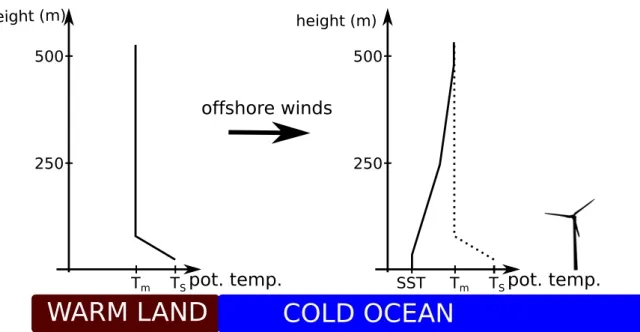
Given the close proximity of o↵shore wind farms to the coast, the MABL at o↵shore wind farms is influenced by the shore. Well known are stable conditions at o↵shore sites caused by the interaction of ocean and the ambient shore during spring and early summer. During daytime, the sea surface temperature (SST) is relatively constant due to the high heat capacity of water. In contrast, the ambient shore warms rapidly and causes an unstable stratification close to the ground (Fig. 3) (Smedman et al. 1997).
In case of o↵shore winds, warm air stemming from the land upwind is advected over the ocean. The advection of warm air associated with a cold SST causes a neutral layer close to the surface followed by a stable internal boundary layer over the ocean, rooted in a turbulent transport of heat towards the ocean resulting in a more pronounced cooling of the air close to the ocean’s surface (e.g. Smedman et al. 1996, 1997; Melas 1998; Lange et al. 2004; Sathe et al. 2011) as indicated in Fig. 3. According to the simulations of Smedman et al. (1997), the neutral layer grows with increasing distance to the shore, resulting in a strengthening of the capping inversion. According to Emeis (2010b), such conditions are favorable for long wakes of o↵shore wind farms.
Another mesoscale phenomenon influencing o↵shore regions in the vicinity of coasts
are sea breeze systems (e.g. Simpson 1994; Miller et al. 2003). The di↵erential heating of land and water bodies results in a pressure gradient, pointing towards the open sea during day time and vice versa during night time. Therefore, a mesoscale system develops that is known as sea breeze. In the literature, three di↵erent sea breeze types are described (Miller et al. 2003). The most prominent type is the pure sea breeze type, where the gradient wind is pointing o↵shore whereas the sea breeze blows onshore. As the gradient wind depends on the dominating synoptic system, the gradient wind is not always orientated perfectly perpendicular to the shoreline (Miller et al.
2003). Therefore, di↵erent types of sea breeze systems exist depending on the shape of the shore and the prevailing wind direction (Steele et al. 2012, 2015). Sea breeze systems can propagate up to 200 km o↵shore (Steele et al. 2015). Consequently, sea breeze systems influence the wind speed and direction at most o↵shore sites according to Fig. 2.
Besides the temperature di↵erence between on- and o↵shore regions the surface roughness at the shore can have an impact on the wind speed over the ocean during stable stratifications. D¨ orenk¨ amper et al. (2015) showed that the varying surface roughness at the coast is responsible for jet streaks close to the surface, propagating more than 100 km o↵shore during stable conditions i.e. resulting from warm air ad- vection as sketched in Fig. 3. Consequently, the surface roughness at the shore can influence the energy harvesting o↵shore during stable conditions.
1.1.2 Wind speed deficit in the far-field of o↵shore wind farms
Due to the large size of o↵shore wind farms and the low turbulence o↵shore, wakes of wind farms are longer o↵shore than onshore. Satellite and aircraft observations have revealed that o↵shore wakes can be longer than 50 km (Hasager et al. 2015; Platis et al. 2018). According to analytical models (e.g., Frandsen et al. 2006; Emeis 2010b), the length of wakes is driven by the vertical momentum flux above wind farms.
Wind turbines extract kinetic energy from the mean flow and convert it partly into
electrical energy. The resulting wind deficit downwind is balanced by the advection of
momentum of the mean flow and the turbulent momentum fluxes. Within large wind
farms, the kinetic energy deficit is mostly balanced by the vertical momentum flux
as the inner turbines are surrounded by wind turbines extracting the kinetic energy
from the mean horizontal flow. Therefore, the wind speed reduction caused by the
wind turbines upwind can only be balanced by the vertical momentum flux. Given the
generally low mean vertical velocities, the turbulent vertical momentum flux determines
the length of the wakes. However, the intensity of vertical momentum flux is directly
related to the turbulence that in turn is known to be lower for o↵shore sites than for
onshore sites. Consequently, wakes o↵shore are longer than wakes onshore (Emeis
2018).
1.1. STATE OF THE ART 5
Figure 2: Distance to coast and average water depth of wind farms under construction in 2017.
(Taken from WindEurope (2017))
Obviously, the wind energy industry has a great interest in forecasting the length of such wakes for economical reasons. Nygaard (2014) and Nygaard and Hansen (2016) showed that a downwind located wind farm produced less energy than the wind farm located upwind. In the US, Miller and Keith (2018b) showed, based on measurements, that wakes of single wind turbines and wind farms decrease the power density of wind farms below 1 W m
2, agreeing with results conducted on a global scale based on simulation of Miller et al. (2015); Volker et al. (2017).
Consequently, such aspects have to be considered during the planning process
and the operation of a wind farm. Given the interest of stakeholders in wakes, a lot
of simulations were conducted, exploring wakes on all scales. Simulations based on
large-eddy simulations (LES) models, investigating the wakes of single wind turbines
within a wind farm were executed in the past (e.g., Calaf et al. 2010, 2011; Port´ e-
Agel et al. 2011; Wu and Port´ e-Agel 2015; Vanderwende et al. 2016; Xie and
Archer 2017). However, simulations covering the scales of a single wind turbine
are computational too expensive to investigate the interaction of several wind farms.
WARM LAND COLD OCEAN
pot. temp.
height (m) 500
250
offshore winds
T
mT
Spot. temp.
500
250
T
mT
SSST
height (m)
Figure 3: Schematic sketch of the evolution of a stable stratification over the ocean caused by warm air advection. T
mand T
Sare the potential temperatures within the mixed layer and of the land surface, respectively. (This figure is based on the simulation and observational results of Smedman et al. (1997). The wind turbine icon is taken from https://svg-clipart.com/white/Ta0k2H4-wind- turbine-clipart.)
Therefore, the wind industry favors simple engineering models because of their low computational cost. A commonly used model is the Park model based on the theory of Jensen (1983), suited to represent the wakes of several single wind turbines, but not for representing deep-array e↵ects, i.e. when an internal boundary layer develops due to intensive mixing within very large wind farms. Consequently, the Jensen model underestimates wake losses downwind of the third row when applying the model to large o↵shore wind farms (Beaucage et al. 2012). Therefore, more sophisticated industrial models combine boundary layer models with single wind turbine wake models to cover the interactions on wind turbine and wind farm scale (Brower and Robinson 2012).
All these industrial models do not account for atmospheric stability although Emeis
(2010b) showed by using an analytical model that the wakes of o↵shore wind farms are
significantly longer during stable conditions. In contrast, mesoscale models represent
atmospheric stability. Such models have a horizontal grid size in the order of one
kilometer. Consequently, mesoscale models do not resolve the e↵ect of a single wind
turbine on the atmosphere explicitly. However, it is possible to represent wind farms in
mesoscale models by the use of parameterizations. In former studies, wind farms were
represented as an area of increased surface roughness (e.g., Ivanova and Nadyozhina
2000; Keith et al. 2004; Wang and Prinn 2010, 2011), a popular approach especially
for global climate simulations (Keith et al. 2004) as no additional computational
resources need to be applied. However, this surface roughness based approach causes a
too weak momentum deficit downwind of the wind farms during nocturnal conditions
1.1. STATE OF THE ART 7
(Fitch et al. 2013).
Nowadays, wind farms are represented as an elevated momentum sink for the mean flow in mesoscale models (e.g. Fitch et al. 2012; Volker et al. 2015). Fitch et al.
(2012) adds turbulent kinetic energy (TKE) at rotor height, representing the additional TKE introduced by the wind turbines. In contrast, Jacobson and Archer (2012) and Volker et al. (2015) let the TKE evolve based on the resolved shear instead of adding TKE directly. Some studies showed that the amount of TKE that is introduced by the parameterization of Fitch et al. (2012) is too excessive (e.g., Abkar and Port´ e- Agel 2015; Volker et al. 2015; Pan and Archer 2018). Therefore, Abkar and Port´ e-Agel (2015) and Pan and Archer (2018) introduced updates to the wind farm parameterization (WFP) of Fitch et al. (2012). In both studies, the authors use LES simulations to account for geometric e↵ects within one grid cell (i.e. staggered vs. unstaggered wind farm) and wind direction. Additionally, they introduce a TKE source, that is also based on the LES results. However, this approach is computationally expensive as the LES results are not transferable to wind farms with a di↵erent layout.
Additionally, the number of necessary LES simulations is the product of the number of wind farms, number of wind directions and atmospheric conditions and, hence, computationally expensive. Further, the WFP of Pan and Archer (2018) has the disadvantage that all wind turbines of a wind farm need to be within one grid cell, meaning that the wind farm size determines the simulation’s horizontal grid.
1.1.3 Micrometeorological, regional and global climate impacts of onshore and o↵shore wind farms
Wind farms can impact the boundary layer. They represent an artificial source of turbulence, resulting in an enhanced mixing of the boundary layer at rotor area but also below and above rotor area. As measurements below and downwind of onshore wind farms are easy to realize compared to o↵shore sites, recently published studies based on observations focused on the impact of onshore wind farms on surface air temperature and soil moisture. Several studies showed that additional mixing at onshore wind farm sites was accompanied by a warming at the surface under stable conditions (e.g., Roy and Traiteur 2010; Zhou et al. 2012; Rajewski et al. 2013; Smith et al. 2013;
Rajewski et al. 2014; Armstrong et al. 2016). For example, Roy and Traiteur (2010) and Armstrong et al. (2016) observed a warming of ⇡ 0.2 K downwind of onshore wind farms at 5 m and 2 m, respectively, especially during nocturnal stable conditions. In contrast, a cooling of ⇡ 1 K was measured by Roy and Traiteur (2010) during daytime. Therefore, the implications of onshore wind farms on agriculture are discussed (e.g., Roy and Traiteur 2010; Rajewski et al. 2013; Smith et al. 2013;
Zhang et al. 2013).
Only a few observational studies focused on the impact of o↵shore wind farms on
the MABL. These studies are all based on photos - except Foreman et al. (2017) and Boettcher et al. (2015), showing fog formation and dispersion due to the enhanced mixing of the wind farm at Horns Rev (Emeis 2010a; Hasager et al. 2013, 2017).
The measurements of Foreman et al. (2017) taken at FINO1, a stationary tower located in the North Sea, revealed that the enhanced mixing in turn, has an influence on the sensible heat flux during stable conditions. Boettcher et al. (2015) simulates a change in cloud cover in the vicinity of Hamburg associated with the installation of wind farms in the North Sea. However, these results are based on simulation using a WFP that was so far not evaluated with observations.
Also, studies based on simulations report an impact of wind farms on the atmo- spheric boundary layer. Regional climate simulations for Europe obtained a significant change in temperature and precipitation in the order of ± 0.3 and 0-5 % (Vautard et al. 2014), respectively. These changes are most significant during the winter sea- son and were partly attributed to local and large-scale e↵ects. In contrast, Pryor et al. (2018a,b) found a significant impact of wind farms in Iowa only during the sum- mer season, with a maximal temperature di↵erence of 0.5 K. These conflicting results arise either from the di↵erent climates of Europe and Iowa and/or the di↵erent hor- izontal grid size they used in their simulations (i.e. 50 km vs. 4 km) (Pryor et al.
2018b). A third study of Sun et al. (2018) investigating the impact of onshore wind farms in China, concludes that wind farms have a significant impact during winter and summer. They observed mainly a temperature increase during winter and a warming during summer at the east coast of China associated with a cooling inland, whereby the impact did not exceed the interannual climate variability (Sun et al. 2018).
Compared to studies based on measurements and regional simulations, global sim-
ulations allow an investigation of the impact of wind farms on the global atmospheric
circulation. Although Wang and Prinn (2011) covered large o↵shore areas with wind
farms (i.e. all o↵shore sites with a water depth below 600 m between 60 S and 74 N),
they observed only weak non-local impacts due to the presence of wind farms. However,
they parameterized the wind farms as areas of increased surface roughness. According
to Fitch et al. (2013), this kind of approach is not suitable to investigate the impact
of wind farms on the climate as this approach overestimates the temperature change
during nocturnal conditions. In contrast to Wang and Prinn (2011), Possner and
Caldeira (2017) obtained surface temperature di↵erences in the order of up to ⇡ 15 K
a↵ecting an area expanding from Iceland to Svalbard when installing a wind farm with
an unrealistic size of 0.67 ⇤ 10
6km
2(equal to two times the size of Germany) in the
North Atlantic, south of Iceland. In general, the installation of large renewable energy
power plants in extreme environments seems to have the biggest impact on atmospheric
circulation. Recently, Li et al. (2018) showed that the installation of wind and solar
power plants in the Sahara Desert would lead to increased temperatures and a doubling
1.2. OPEN QUESTIONS AND OBJECTIVES OF THE PRESENT STUDY 9
of the precipitation in the Sahel region due to enhanced surface friction and reduced albedo. Given the potentially large impact of o↵shore wind farms, Pan et al. (2018) investigated whether a wind farm could reduce the hurricane thread along the coast of the Gulf of Mexico. They showed that wind farms could have reduced the precipitation and wind speed at hub height by 100 mm and 5 m s
1, respectively, during hurricane Harvey.
Similar to mountains, wind farms impose an obstacle to the atmospheric flow and perturb the pressure field, hence, wind farms can trigger gravity waves. Due to conservation of mass, this pressure perturbation results either in an acceleration at the flanks of a wind farm and/or an enhanced flow over the wind farms, equal to a vertical lift for air parcels going over the wind farm. During stable conditions, this lift can cause gravity waves as it is described in Smith (2010) and Allaerts and Meyers (2018).
They both suggest that gravity waves are most likely to be observed in atmospheres with a Froude number close to unity. However, Smith (2010) concluded that a low surface drag with a Froude number close to unity causes a strong blocking and, hence, an increased extinction of gravity waves. In contrast, Allaerts and Meyers (2018) found that a low surface drag plays a minor role in generating gravity waves.
1.2 Open questions and objectives of the present study
Mesoscale wind farm parameterizations (WFP) need to be evaluated for o↵shore re- gions. The performance of WFPs for mesoscale models has been so far only investi- gated either in idealized simulations (e.g., Volker et al. 2015; Chatterjee et al.
2016; Vanderwende et al. 2016) or for onshore sites Lee and Lundquist (2017) - except Jim´ enez et al. (2015) and Hasager et al. (2015). Jim´ enez et al. (2015) evaluated the WFP of Fitch et al. (2012) by the use of energy production data of a single o↵shore wind farm (Horns Rev) o↵ the Danish coast. Consequently, they were not able to evaluate the spatial dimensions of the wake of the Horns Rev wind farm.
Taking into account that more wind farms are planned to be built in the North Sea, resulting in shorter distances between the wind farms, the spatial scales of wakes are of major interest for wind energy stakeholders. Additionally, idealized simulations ne- glect moisture e↵ects and assume a neutral stratification with a uniform upwind inflow, although o↵shore wind farms are exposed to stable conditions and topographic e↵ects introduced by the coast (see section 1.1.1). Consequently, measurements are needed to evaluate the performance of WFPs in real case simulations.
Additionally, although there is disagreement over to whether or not use an ad- ditional TKE source in WFPs, the simulated impact on the marine atmosphere has not been evaluated for real case studies. Several studies based on simulations suggest (e.g., Eriksson et al. 2015; Vanderwende et al. 2016) that the WFP of Fitch et al.
(2012) adds too much TKE into the model causing exaggerated mixing. However, the
TKE and the associated change in the vertical fluxes over wind farms is difficult to evaluate, especially for o↵shore wind farms due to their remote locations. Therefore, implications of mesoscale WFPs on the TKE were so far not evaluated although they are of major importance when estimating the impact of large o↵shore wind farms on the MABL.
The uncertainty considering the TKE source of WFPs, could lead to wrong mesoscale wake simulations. According to analytical models, the impact of large o↵- shore wind farms is rooted in an enhancement of the vertical fluxes above wind farms (Emeis et al. 2016). As some boundary layer parameterizations (e.g. Nakanishi and Niino (2006)) calculate the vertical fluxes diagnostically based on the TKE, a careful evaluation of TKE over the wind farms is necessary before the simulated wakes can be evaluated.
Summarized, it is not clear whether WFPs can simulate realistic wakes under stable conditions when the impact on the MABL is expected to be largest, as the optimal configuration of the WFP is not known, i.e. with or without a TKE source and with which resolution of the driving mesoscale model. Consequently, assessments of the regional climate impact of o↵shore wind farms based on mesoscale simulations have a large uncertainty.
wind farm scale 100 m - 10 km
wake scale 1 km - 100 km
regional scale 20 km - 250 km
small
intermediate
Figure 4: The bottom-up approach of this PhD thesis. The WFP of Fitch et al. (2012) is evaluated on a wind farm and wake scale before the impacts on the regional climate are investigated. (The wind turbine icon is taken from https://svg-clipart.com/white/Ta0k2H4-wind-turbine-clipart.)
This study evaluates the impacts of the WFP of Fitch et al. (2012) on the MABL at wind farm (100 m – 10 km) and wake (1 km – 100 km) scale to provide a sound basis for investigating impacts on the regional scale (20 km – 250 km) as sketched in Fig. 4.
Summarized, this thesis starts from an analysis of small-scale processes (wind farm) via an intermediate scale (wake) to an assessment of impacts of o↵shore wind farms on the regional scale. First of all, the TKE of mesoscale simulations above o↵shore wind farms is compared to airborne measurements as the TKE is driving the vertical fluxes i.e. the wind farm scale. Secondly, we evaluate the impacts of large o↵shore wind farms in the far-field
1of o↵shore wind farms i.e. the wake scale. Based on these
1
By far-field we refer throughout the whole manuscript to the area 5 km and more downwind of a
1.2. OPEN QUESTIONS AND OBJECTIVES OF THE PRESENT STUDY 11
evaluation results it is possible to discuss potential impacts of o↵shore wind farms on the regional scale - the largest scale considered in this thesis (Fig. 4). More specifically, we try to answer the following questions:
• How to configure the WFP of Fitch et al. (2012) and the driving mesoscale model to represent the impact of o↵shore wind farms on TKE and wind speed above wind farms?
• Is it possible to correctly simulate the far-field of large o↵shore wind farms with the setup obtained above?
• What are the micrometeorological and regional climate impacts of o↵shore wind farms?
In chapter 2 we describe the aircraft measurements and the simulations used to answer the questions pointed out above. The first two questions are treated in the chapters 3 and 4 to have a sound basis for the discussion about potential regional climate impacts of o↵shore wind farms on the MABL and the land located downwind of large o↵shore wind farm clusters (chapter 5).
wind farm
This chapter presents the data we used for analyzing and evaluating our simulations, including aircraft measurements, synthetic aperture radar (SAR) data, ground-based observations and reanalysis data (sections 2.1, 2.2, 2.3 and 2.4). This is followed by an explanation of the WFP of Fitch et al. (2012) (section 2.5), with a description of the driving mesoscale model (section 2.6). An overview of the wind farms implemented in the mesoscale model is given in section 2.7. This chapter is based on the data and method descriptions as presented in Siedersleben et al. (2018a, 2019).
2.1 Aircraft observations
This section presents aircraft observations that were executed with the aircraft Dornier 128-6, operated by the TU Braunschweig. Three kinds of aircraft observation were conducted within the framework of this study: vertical profiles upwind of o↵shore wind farms (section 2.1.2), the measurements recorded within the far-field of wind farms (section 2.1.3) and flights performed above wind farms (section 2.1.4). The uncertainties in the aircraft measurements are explained in section 2.1.1.
2.1.1 Uncertainties in the aircraft measurements
The aircraft measurements have two kinds of errors - a systematic and a relative error.
The systematic error is rooted in the accuracy of the sensor itself. The temperature sensor has an accuracy of 0.2 K (Corsmeier et al. 2001), and the wind speed mea- surements an accuracy of 0.5 m s
1with a resolution of 0.08 m s
1(Br¨ ummer et al.
2003). The relative error is rooted in the size of the eddies of the atmosphere and, hence, the measurement strategy, as the error is a direct function of the sampling length (Mann and Lenschow 1994). The airborne measurements are area-averaged over 300 and 3000 data points for the climb flights and for the horizontal flight patterns corresponding to 30 m and 2 km, respectively. By averaging over di↵erent length scales we systemically under- or overestimate the turbulent values and standard deviations of temperature and wind speed. Following Mann and Lenschow (1994), we have a relative error of 10 % during the climb flights and 1 % during the horizontal flight pat- terns (i.e. above and downwind of the wind farms) for the wind speed measurements (Platis et al. 2018). The temperature observations have a relative error of 0.015 K during the climb flight. As we use area averages in our data analysis to investigate the spatial variation of temperature and wind measurement, the relative error is applicable.
The corresponding Gaussian error propagation for the wind direction is ± 3 . 2.1.2 Vertical profiles
To be aware of the atmospheric flow conditions and to provide a sound basis for the model evaluation, the aircraft probed the atmosphere in the vicinity of the wind farms
12
2.1. AIRCRAFT OBSERVATIONS 13
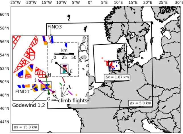
Figure 5: Locations of WRF domains and wind farms at the North Sea. A close-up on the German Bight shows the wind farms of interest framed with gray rectangles and the flight tracks above the wind farms in black, green and magenta, corresponding to the measurements executed on 09 August 2017, 14 and 15 October 2017, respectively. All measurements over the wind farms have a start and end point indicated with a capital letter for better orientation in Fig. 14, 16 and 18. Blue wind farms are in use, orange wind farms are approved or under construction according to plans in 2017, wind farms plotted as red polygons are potential areas for wind farms according to plans in 2015. The gray dashed rectangle highlights the location of the observations executed on 10 September 2016 with the wind farms Meerwind Sued Ost (gray), OWP Nordsee Ost (green) and Amrumbank West (purple) shown in detail in Fig. 6. The thick lines indicate the locations of the climb flights, whereby the coloring corresponds to the coloring of the flight tracks over the wind farms, except the light red and red star showing the locations of the two additional profiles recorded before and after the two additional flight legs on 15 October 2017 and the brown thick line indicating the location of climb flight on 10 September 2016. A detailed look at the wind turbine distribution of the wind farms of interest is provided in Fig. 7. The wind turbine location data was provided by the German Federal Maritime and Hydrographic Agency (BSH) and Bundesnetzagentur (2017).
of interest to obtain vertical profiles of the atmosphere during each observation. In
this thesis, we present six vertical profiles in detail, the locations of these profiles are
shown in Fig. 5 and the corresponding dates and times are given in Table 1.
Table 1: Date and start time of climb flights in the vicinity of wind farms. The corresponding locations are shown in Fig. 5
Date Time (UTC) color, marker in Fig. 5 10 September 2016 08:00 brown thick line
09 August 2017 13:22 black thick line 14 October 2017 13:22 green thick line 15 October 2017 07:17 magenta thick line 15 October 2017 9:23 light red star
15 October 2017 10:18 red star
2.1.3 In the far-field of o↵shore wind farms
The research aircraft flew two di↵erent flight patterns to capture the vertical and horizontal extent of wakes in the far-field. In particular, we will focus on measurements recorded on 10 September 2016, all other flights with such a pattern are listed in Table 2.
The horizontal flight pattern on 10 September 2016 is shown in Fig. 6 with flight legs perpendicular to the mean wind speed at hub height equal to 90 m AMSL. The first flight leg was flown 5 km downwind of the wind farm. Four further flight legs 15 km, 25 km, 35 km and 45 km downwind of the wind farms were also flown. Note these measurements took more than 1 hour.
Additionally, the vertical extent of the wake 5 km downwind of the wind farm cluster Amrumbank West was observed on 10 September 2016 by 5 flight legs at 5 di↵erent heights along the cross-section A-B (Fig. 6): 60 m, 90 m, 120 m, 150 m and 220 m AMSL. The vertical flight pattern took place from 1000 UTC to 1100 UTC, we present this data in chapter 4.
2.1.4 Above o↵shore wind farms
Three sets of aircraft observations were executed above o↵shore wind farms, labeled as case I, II, and III, summarized in Table 3. The aircraft observations were conducted on 09 August (case I), 14 October (case II) and 15 October 2017 (case III) at two di↵erent wind farm clusters (Fig. 5, Fig. 7). The observations on 09 August 2017 and 14 October 2017 started at ⇡ 14:15 UTC and lasted 35 minutes and 52 minutes.
The measurements on 15 October 2017 took place from 14:15 UTC to 09:21 UTC and 09:52 UTC to 10:17 UTC. The di↵erent observational periods are summarized in Table 3.
All aircraft measurements have the same pattern. Before we started the measure-
ments over the wind farms, the aircraft profiled the MABL in the vicinity of the wind
farms of interest, followed by several flights over the wind farms orientated perpendic-
ular to the large scale synoptic forcing. During all observations, the aircraft overflew
the wind farm at least four times. Case study III included two additional measure-
2.1. AIRCRAFT OBSERVATIONS 15
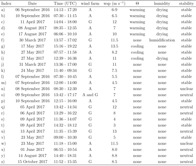
Table 2: Overview of flights conducted within the WIPAFF project downwind of large o↵shore wind farms. The numbering of the aircraft measurements corresponds to the numbering in Fig. 29 and in Fig. 30. The letters A and G indicate the measurement location; A refers to the wind farm cluster consisting of Amrumbank West, Meerwind S¨ ud Ost and Nordsee Ost and G for the wind farm Godewind. The locations of these wind farms are indicated in Fig. 5. The column indicated with wsp, shows the measured wind speed at hub height according to Fig. 29. The sixth and seventh column indicate whether the wind farms had an impact on temperature or humidity at hub height downwind.
The atmospheric stability during each measurement is shown in the last column according to the potential temperature gradient within the rotor area shown in Fig. 29. Observations where wind farms had an impact on the atmosphere are listed at the beginning of the table. The observations suggest that a wind speed over 6 m s
1and stable conditions are a sufficient constraint to observe warming or cooling. The cases fulfilling these criteria are the cases (a-k). The reasons why no warming or cooling was observed in the cases f, j and k is discussed in chapter 4 section 4.4.2.
Index Date Time (UTC) wind farm wsp (m s
1) ⇥ humidity stability
a) 06 September 2016 14:13 - 17:20 A 6-9 warming drying stable
b) 10 September 2016 07:30 - 11:15 A 6.5 warming drying stable
c) 11 April 2017 14:04 - 18:00 G 12 warming drying stable
d) 08 August 2017 08:35 - 12:35 A 7 warming drying stable
e) 17 August 2017 06:06 - 10:10 A 10 warming drying stable
f) 30 March 2017 13:57 - 17:02 G 11.5 none humidification stable
g) 17 May 2017 15:16 - 19:22 A 13.5 cooling none stable
h) 27 May 2017 07:57 - 11:58 A 8.2 cooling none stable
i) 27 May 2017 12:39 - 16:36 A 11 cooling drying stable
j) 31 March 2017 13:36 - 17:00 G 11 none none stable
k) 24 May 2017 11:40 - 09:34 G 7.5 none none stable
l) 07 September 2016 07:30 - 10:45 A 5.5 none none stable
m) 07 September 2016 12:00 - 14:00 A 4.5 none none stable
n) 08 September 2016 08:30 - 12:30 A 7 none none unclear
o) 09 September 2016 13:42 - 17:17 A and G 7 none none neutral
p) 10 September 2016 12:15 - 16:00 A 4.5 none none stable
q) 05 April 2017 13:42 - 14:34 G 12 none none neutral
r) 06 April 2017 13:29 - 16:22 G 8 none none neutral
s) 09 April 2017 11:36 - 14:07 G 4 none none stable
t) 09 April 2017 14:32 - 18:12 G 3 none none stable
u) 13 April 2017 11:35 - 15:39 G 13 none none neutral
v) 23 May 2017 09:00 - 10:30 G 5 none none stable
w) 23 May 2017 11:18 - 15:00 A 11.5 none none unclear
x) 01 June 2017 06:55 - 10:54 A 8.0 none none neutral
y) 14 August 2017 14:40 - 18:31 A 8.8 none none neutral
z) 15 October 2017 11:52 - 15:35 G 8.5 none none neutral
ments over the wind farms of interest conducted 40 min after the first four flight legs (Table 3).
The measurements were executed at two di↵erent wind farms (Fig. 5) with two
di↵erent rotor types (more details in section 2.7). Therefore, di↵erent flight heights
were necessary - the aircraft flew at 200 m AMSL for case study I and 250 m AMSL
Amrumbank West OWP Nordsee Ost Meerwind SuedOst
DanTysk Butendiek
large scale flow
flight track at hub height
10 km
45 km
A B
Figure 6: The wind farms of interest, the flight track of the research aircraft with time stamps in UTC and the mean wind direction during the field campaign on 10 September 2016. A gray dashed box in Fig. 5 indicates the location of the shown close-up. Every single wind turbine is plotted as a dot and the corresponding wind farms Meerwind SuedOst (MSO, green dots), OWP Nordsee Ost (ONO, orange dots), Amrumbank West (AW), Butendiek and DanTysk are annotated in the Figure. The flight track is indicated with a black solid line. The orientation of the wind direction on 10 September 2016 at 09:00 UTC is denoted by an arrow.
Table 3: Location, date and time of aircraft observations above wind farms
Case study Date Time (UTC) number of flight legs wind farms
I 09 August 2017 14:14 - 14:51 4 Meerwind SuedOst, OWP Nordsee Ost
II 14 October 2017 14:19 - 15:11 4 Godewind 1, 2
III 15 October 2017 8:28 - 9:21 4 Godewind 1, 2
15 October 2017 9:52 - 10:17 2 Godewind 1, 2
for case study II and III, over the wind farms (Fig. 8) Meerwind S¨ ud Ost (MSO) and OWP Nordsee Ost (ONO), Godewind 1,2 (GW), respectively.
2.2 Synthetic Aperture Radar Data (SAR)
Satellite data from Sentinel-1A is used to evaluate the orientation of the simulated wakes for the 14 October 2017. Literature published in the past has shown that Syn- thetic Aperture Radar (SAR) is a powerful tool to detect wakes o↵shore (e.g., Chris- tiansen and Hasager 2005; Li et al. 2014; Hasager et al. 2005, 2015; Djath et al.
2018), due the reduced surface roughness within the wakes, rooted in the wind speed deficit downwind of o↵shore wind farms, resulting in turn in an altered backscattering at the sea surface. By applying post-processing methods as suggested by Djath et al.
(2018), the back scattered signal can be used to calculate the wind speed at 10 m height.
2.3. GROUND-BASED OBSERVATIONS 17
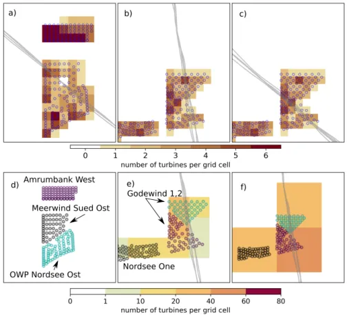
d) e) f)
b) c) a)
Meerwind Sued Ost Amrumbank West
OWP Nordsee Ost
Godewind 1,2
Nordsee One
Figure 7: The number of wind turbines within one grid cell in colored contours for the wind farms (a) Meerwind Sued Ost and OWP Nordsee Ost and (b-c) Godewind 1, 2 for the control simulations (CN- TRa, CNTRb, CNTRc). The size of the contour areas corresponds to the size of the horizontal model grid. The circles denote the exact locations of the single wind turbines whereby the wind turbines are colored according to the wind farm they belong to in (d-f), additionally (e-f) show the horizontal grid with 5 km and 16 km resolution for the sensitivity studies: DX5, DX16, noTKEsourceDX5 and noTKEsourceDX16. The wind turbines are not colored in (a-c) for better visibility of the wind turbine density. The gray lines denote the flight track of the research aircraft.
However, these methods assume neutral wind conditions (Verhoef et al. 2008), hence, we only use the data of Sentinel-1A taken at 17:17 UTC on 14 October 2014 to evaluate the orientation of the simulated wakes and not the wind speed.
2.3 Ground-based observations
To evaluate the simulations for the 10 September 2016 we use ground-based observa-
tions of the measurement towers FINO1 and FINO3. These towers are used to assess
the lower marine atmosphere, up- and downwind of the wind farms of interest (location
of towers is shown in Fig. 5) as the aircraft can not measure below 60 m AMSL. In con-
trast to the sounding of Norderney, FINO1 and FINO3 have the advantage that they
are not influenced by the land surface and, hence, give a representative stratification
of the marine boundary layer below hub height. Moreover, FINO3 was not influenced
by any wakes due to the south-westerly winds on 10 September 2016. In contrast,
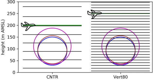
Figure 8: Distribution of the vertical levels with height and the levels intersecting with the rotor areas of the two wind turbine types used in the wind farms as listed in Table 5 for the CNTR and the Vert80 simulation. The rotor areas of the wind turbine SIEMENS-SWT-6.0-154 and SIEMENS SWT 3.6-120 are shown in magenta and blue, respectively. The green lines denote flight heights at 200 m and 250 m AMSL; necessary due to the two di↵erent wind turbine types. The aircraft icon is taken from https://www.trzcacak.rs.
FINO1 was likely influenced by Borkum Ri↵grund 1. Therefore, the temperature and wind measurements at FINO1 have to be used with caution. FINO1 is equipped with five temperatures sensors at 33 m, 50 m, 70 m, 90 m and 100 m AMSL, whereas FINO3 has only 3 temperature sensors at 50 m, 70 m, and at 90 m AMSL (Neumann et al. 2004). The temperature sensors at FINO1 have an absolute accuracy of 0.5 K (R. Fruehmann 2018, personal communication) and agree relative to each other with an accuracy of ± 0.05 K (Fruehmann 2016). The temperature sensors at FINO3 have an absolute uncertainty of 1.21 K (A. Mark 2018, personal communication).
2.4 Reanalysis Data: ECMWF analysis and ERA5 data
We use ECMWF analysis or ERA-interim data to assess the weather on a synoptic scale for all case studies presented in this study. Additionally, both data sets are used to define the lateral and initial boundary conditions of our simulations. ERA5 analysis data is freely available at Copernicus Climate Change Service (C3S) (2018) with a horizontal resolution of 0.25 degrees whereas ECMWF analysis data having a grid size of 0.125 degrees and has restricted access.
2.5 Wind farm parameterization
In this thesis all simulations use the wind farm parameterization of Fitch et al. (2012).
This parameterization acts as an elevated momentum sink for the mean flow and a
2.6. NUMERICAL SETUP 19
source of turbulence, depending on the thrust - and power coefficient C
Tand C
P. Both coefficients are a function of wind speed and are di↵erent for every wind turbine type - an example for the wind turbine type SIEMENS SWT 3.6 120 onshore
1is shown in Fig. 9. The power coefficient is the electrical power P
egenerated by a wind turbine normalized by the power of the wind:
C
P= P
eP
wind. (2)
However, the power coefficient can also be used to describe the rate of loss of kinetic energy from the atmosphere associated with the conversion of kinetic into electrical energy (Fitch et al. 2012). The thrust coefficient C
Tdescribes the total fraction of energy that is extracted by a single wind turbine from the atmosphere (Fitch et al.
2012). The amount of energy that is not converted into electrical energy is lost due to frictional and electrical losses and non-productive drag. In the parameterization of Fitch et al. (2012) frictional and electrical losses are neglected, hence, all losses are caused by non-productive drag, that in turn produces turbulence. Consequently, the di↵erence between C
Tand C
Pdescribes the fraction of energy converted into TKE.
More specifically, the amount of TKE added to the model is:
@T KE
ijk@ t =
1
2
N
tijC
T KEV
ijk3A
ijkz
k+1z
k(3)
C
T KE= C
T(V
H) C
P(V
H) (4) whereby C
T KEdescribes the fraction of energy converted into TKE. Equation 3 is formulated for a Cartesian coordinate system with the indexes i, j, k corresponding to the directions x, y, z, that, in turn, is equal to the geographic directions West-East, South-North, and the vertical axis with k=0 the level closest to the ground. The variable N
ijdescribes the wind turbine density within a grid cell i, j having the units m
2; V
ijkis the horizontal wind speed at grid cell ijk; A
ikjis the rotor area between the two vertical levels k and k + 1, at a height z
kand z
k+1, and V
Hthe horizontal wind speed at hub height. Consequently, the rate of change in TKE is highest for high wind speeds, a large number of wind turbines within one grid cell and a large di↵erence between the power and thrust coefficient.
2.6 Numerical Setup
In this thesis, we present simulations covering 10 September 2016, 09 August 2017 and 14, 15 October 2017. For all these days we performed simulations using the control configurations as described in section 2.6.1. The control simulations covering the 09 August 2017 and 14, 15 October 2017 are named CNTRa, CNTRb and CNTRc
1
data available at: http://www.wind-turbine-models.com/turbines/646-siemens-swt-3.6-120-
onshore, accessed on 5th December 2017
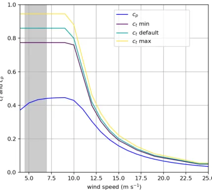
Figure 9: Thrust- and power coefficient c
tand c
pof the wind turbine SIEMENS SWT 3.6 120 onshore.
The c
pvalues used in the sensitivity experiments c
pmin and max are shown in purple and yellow.
throughout this thesis. Additionally, we executed simulations with di↵erent setups to investigate the sensitivity of our simulations with a focus on 14 October 2017. The di↵erent configurations of the sensitivity simulations are presented in section 2.6.2.
2.6.1 Control configuration
All simulations are conducted with the Weather Research & Forecasting Model WRF, version 3.8.1 (ARW, Skamarock et al. (2008)). The model uses three domains with a horizontal grid size of 15 km, 5 km and 1.67 km, respectively. The location of the two way nested domains are shown in Fig. 5. The time step is 60 s for the coarsest domain, 20 s and 5 s for the following domains, respectively.
The initial and lateral boundary conditions are defined with operational ECMWF analysis data in 6 hourly intervals for the simulations covering the 10 September 2016, as we obtained best results with this data for this specific day. For all other simulations, we use ERA-interim reanalysis data (Copernicus Climate Change Service (C3S) 2018) with a resolution of 0.25 degree in 6 hourly intervals
2.
The SST a↵ects the stratification of the atmosphere, hence, mesoscale simulations with refined SST data (such as that provided via the Operational Sea Surface Tem- perature and Sea Ice Analysis (OSTIA) product), can improve mesoscale simulations (Shimada et al. 2015). However, the SST data from OSTIA for the case studies
2
ERA-INTERIM reanalysis data is freely available via the Copernicus Climate Change Service
Climate Data Store, hence, the majority of boundary conditions were provided by ERA-interim data
2.6. NUMERICAL SETUP 21
presented here only di↵er marginally from the SST data provided from ECMWF anal- ysis or the ERA5 data. Therefore, we did not update the SST using an advanced SST dataset. Hahmann et al. (2015) pointed out that boundary layer winds over land have a spin-up time larger than 12 hours and could, therefore, influence o↵shore boundary layer wind climatology. Therefore, our model is initialized at 1200 UTC the day before or in the night before the observations at 00 UTC and integrated over 24 hours (i.e., to have a spin-up of more than 12 hours). This is true for all simulations, except for the simulation conducted for the 15 October 2017, here we only have a spin-up time of nine hours as the additional 6 hours spin-up time showed no improvement considering the vertical representation of the atmosphere.
In the control configuration, we use a vertical spacing of 35 m in the lowest 200 m and increasing to 100 m at 1000 m above mean sea level (AMSL) corresponding to one vertical level below the rotor area and three within the rotor area for the wind turbine type installed at the wind farms MSO and ONO (Fig. 8). Four vertical levels are located within the rotor area for the wind farm GW (Fig. 8) due to the larger rotor area.
The following parameterizations are used in all three domains: the WRF double- moment 6-class cloud microphysics scheme (WDMS; Lim and Hong (2010)), the Rapid Radiative Transfer Model for GCM (RRTMG) scheme for short- and longwave radi- ation (Iacono et al. 2008), the Noah land surface model (Chen and Dudhia 2001) and the Mellor-Yamada-Nakanishi-Niino (MYNN) boundary layer parameterization (Nakanishi and Niino 2006) interacting with the WFP, as described in section 2.5.
In the two innermost domains convection is resolved explicitly, only the first domain uses the cumulus parameterization of Kain (2004).
2.6.2 Sensitivity configurations
Sensitivity simulations were performed for two days: 10 September 2016 and 14 Oc- tober 2017. The simulations covering 10 September 2016 focus on the uncertainty of the wake simulations (section 4.3 in chapter 4) rooted in the estimated thrust and power coefficients of the simulated wind turbines. In contrast, the sensitivity studies conducted for the 14 October 2017 address the question whether an additional TKE source in a WFP is needed to represent the impact of o↵shore wind farms during stable conditions on the MABL. All sensitivity studies executed for 14 October 2017 are listed in Table 4.
Lee and Lundquist (2017) obtained the best results with 80 vertical levels - equal
to a vertical spacing of 12 m below 400 m AMSL. Therefore, we tested the sensitivity
of our results using the vertical levels of Lee and Lundquist (2017) - equal to three
full levels below and ten full levels within the rotor area for the wind farms MSO,
ONO and two full levels and 13 full levels within the rotor area for the wind farms GW
(Fig. 8).
The vertical levels of Lee and Lundquist (2017) demand smaller time steps due to the higher resolution. Therefore, we use 10 s, 3.33 s and 0.67 s corresponding to the three domains. We named the simulations using 80 vertical levels Vert80.
The sensitivity of our results with respect to the horizontal grid size was tested with simulations of 5 km and 16 km horizontal resolution, respectively. Consequently, the number of turbines within one grid cell changes as it is shown in Fig. 7e-f. We obtained best results using a horizontal grid size of 1.67 km.
Recently, some published studies (e.g., Abkar and Port´ e-Agel 2015; Eriksson et al. 2015; Vanderwende et al. 2016; Pan et al. 2018) suggested that the mixing induced by the WFP of Fitch et al. (2012) is too high due to the added TKE into the model (see equation 3). Therefore, we tested the sensitivity of our simulations by switching the TKE source o↵. Three simulations were performed using a horizontal grid spacing of 1.67 km, 5 km and 16 km with a disabled TKE source (noTKEsource, DX5noTKEsource, DX16noTKEsource). As we expect a simulation with more vertical levels to resolve more vertical shear, we performed additionally a simulation using 80 vertical levels with a grid size of 1.67 km and no TKE source (Vert80noTKEsource).
Since WRF version 3.8.1 TKE advection can be activated in the boundary scheme of Nakanishi and Niino (2004). In previously published studies (e.g., Mangara et al. 2019) this option was used. Therefore, we tested the sensitivity of our results with respect to this option.
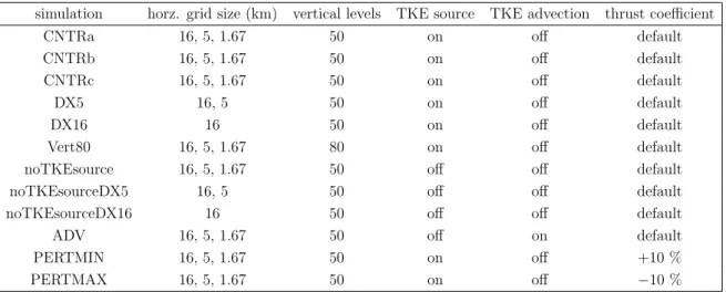
Table 4: Overview of performed numerical simulations and parameter choices for the sensitivity experiments.
simulation horz. grid size (km) vertical levels TKE source TKE advection thrust coefficient
CNTRa 16, 5, 1.67 50 on o↵ default
CNTRb 16, 5, 1.67 50 on o↵ default
CNTRc 16, 5, 1.67 50 on o↵ default
DX5 16, 5 50 on o↵ default
DX16 16 50 on o↵ default
Vert80 16, 5, 1.67 80 on o↵ default
noTKEsource 16, 5, 1.67 50 o↵ o↵ default
noTKEsourceDX5 16, 5 50 o↵ o↵ default
noTKEsourceDX16 16 50 o↵ o↵ default
ADV 16, 5, 1.67 50 o↵ on default
PERTMIN 16, 5, 1.67 50 on o↵ +10 %
PERTMAX 16, 5, 1.67 50 on o↵ 10 %
2.7 Wind farms implemented in the numerical model
The aircraft measurements and simulations presented in this study focus on the wind
farms Amrumbank West (AW), OWP Nordsee One (ONO), Meerwind SuedOst (MSO)
and Godewind 1,2 (GW) (Fig. 5, Fig. 6), hence only these wind farms are presented
2.8. ENERGY BUDGET FRAMEWORK 23
in detail. For all other wind farms installed at the North Sea, the interested reader is referred to Bundesnetzagentur (2017).
Within these wind farms, three di↵erent types of wind turbines are installed: At the wind farms AW and at MSO the wind turbine SIEMENS SWT 3.6-120, having a nominated power of 3.6 MW, a rotor diameter of 120 m and a hub height of 90 m, resulting in a rotor top of 150 m (Fig. 8). The wind turbines at the wind farms ONO and GW (Fig. 6, Fig. 7) have a nominated power of 6.2 MW and 6.0 MW with a hub height of ⇡ 96 m and 110 m, and a rotor diameter of 126 m and 154 m, resulting in a rotor top of 159 m and 187 m, respectively.
For approved and wind turbines currently under construction, i.e. wind turbines colored orange in Fig. 5 (April 2018), we assumed the same wind turbine type as installed at AW, the SIEMENS SWT 3.6-120. The locations of these wind turbines were made available by the German Federal Maritime and Hydrographic Agency (BSH) and Bundesnetzagentur (2017). For potential areas of future wind farms (i.e. red polygons in Fig. 5), the same turbine spacing as at the wind farm AW was assumed - one of the highest wind turbine densities existing at the German Bight.
Table 5: Wind turbine types installed in the model according to the data of the Bundesnetzagen- tur (2017)
.
wind farm wind turbine type hub height (m) diameter (m)
Godewind SIEMENS SWT-6.0-154 110 154
Amrumbank West SIEMENS SWT 3.6-120 90 120 Meerwind SuedOst SIEMENS SWT 3.6-120 90 120 OWP Nordsee Ost SENVION 6.2 95.4-97.04 126
Public information on turbine thrust - and power coefficients is not widely avail- able, and so we also explored the sensitivity of our results to these parameters. We altered the estimated thrust coefficient by ± 10 %, resulting in two simulations (PERT- MIN, PERTMAX) that are expected to introduce more and less TKE into the model than the CNTRb simulation. The results are presented in section 3.3.4. Sensitivity simulations of the same kind were conducted for the 10 September 2017 case study (section 4.3) to investigate the impact of this uncertainty on the far-field.
2.8 Energy budget framework
In chapter 5 this work discusses potential impacts of o↵shore wind farms on the regional climate. Therefore, this section presents a brief overview of the atmospheric energy budget.
According to Porter et al. (2011) the rate of energy change in a vertical column
of the atmosphere is:
@
@t 1 g
Z
psptop
(c
pT + + Lq + k)dp = F
RAD+ F
SF C+ F
W ALL, (5) where c
pis the specific heat capacity of air at constant pressure (1005.7 J K
1), the geopotential, L the latent heat that is released in case of evaporation (2.501 x 10
6J kg
1) and q the specific humidity. The vertical column is integrated from the surface pressure p
sto the top of the atmosphere p
top(in case of a model data analysis p
toprefers to the highest pressure level of the model). Following equation 5, the rate of energy change in the vertical column is determined by the radiation budget at the top of the atmosphere F
RAD, and at the surface F
SF Cand the divergence of energy within the column F
W ALL.
The radiation budget F
RADat the top of the atmosphere is the di↵erence between the net short- and longwave radiation:
F
RAD= F
SWF
LW. (6)
At the surface (i.e. at p
sf c) F
SF Ccan be expanded to:
F
SF C= SW
SF C+ LW
SF C+ Q
H+ Q
E(7) where SW
SF Cand LW
SF Cis the net short- and longwave radiation at the surface.
The third term Q
His the sensible heat flux and Q
Ethe latent heat flux.
The divergence of energy F
W ALLwithin a vertical column can be written as:
F
W ALL= r 1 g
Z
psptop