A stochastic intra-ring synchronous optimal network design problem

(1)

A Stochastic Intra-Ring Synchronous Optical Network Design Problem

?

J. Cole Smith

??

Andrew J. Schaefer

???

Joyce W. Yen

?

Department of Systems and Industrial Engineering University of Arizona, Tucson, AZ 85721

cole@sie.arizona.edu

??

Department of Industrial Engineering University of Pittsburgh, Pittsburgh, PA 15261

schaefer@engrng.pitt.edu

???

Industrial Engineering

University of Washington, Seattle, WA 98195-2650 joyceyen@u.washington.edu

Subject Classifications: Programming: stochastic, integer (applications, Benders/

decomposition).

Area of Review: TELECOMMUNICATIONS.

(2)

Abstract

We develop a stochastic programming approach to solving an intra-ring Synchronous Optical Network (SONET) design problem. This research differs from pioneering SONET design studies in two fundamental ways. First, while traditional approaches to solving this problem assume that all data are deterministic, we observe that for practical planning situations, network demand levels are stochastic. Second, while most models disallow demand shortages and focus only on the minimization of capital Add-Drop Multiplexer (ADM) equipment expenditure, our model minimizes a mix of ADM installations and expected penalties arising from the failure to satisfy some or all of the actual telecommunication demand. We propose an L-shaped algorithm to solve this design problem, and demonstrate how a nonlinear reformulation of the problem may improve the strength of the generated optimality cuts. We next enhance the basic algorithm by implementing powerful lower and upper bounding techniques via an assortment of modeling, valid inequality, and heuristic strategies. Our computational results conclusively demonstrate the efficacy of our proposed algorithm as opposed to standard L-shaped and extensive form approaches to solving the problem.

1 Introduction

The last decade has witnessed a proliferation in the research and development of optical telecommunication fiber. Modern optical fibers typically permit the simultaneous transmission of 2.4 Gbps (gigabits per second) of data over each strand of fiber. Additionally, optical fibers are also preferred over copper wires due to their increased security and maintainabil- ity. Specific advantages and technical details of fiber-optic technology may be found in Wu (1992).

(3)

With the advent of this technology, the failure of a single optical fiber may result in a sub- stantial loss of customer service. Several network topologies, including point-to-point diverse protection (DP) and self-healing ring (SHR) architectures, have been proposed to sustain the survivability of optical networks in the event of equipment failure. These topologies consider a set of nodes, which usually represent voice/data traffic origins and destinations in the network, and a set of arcs that represent connecting fibers. DP topologies enhance network reliability by including protective lines within the network, which can be utilized in the event of a facility failure (either a node or an arc) to re-route traffic. DP networks may be cost-prohibitive if the number of protection lines that must be installed to ensure a desired level of network survivability is too large. By contrast, in SHR architectures, the nodes are connected by a ring of fibers, and traffic routed along the ring is automatically re-routed in the case of equipment failure.

The Synchronous Optical Network (SONET) is a standard of transmission technology used in optical fiber networks designed under SHR topologies (Wu (1992) and Wu and Burrowes (1990) provide an in-depth description of the SONET ring architecture). The costliness of constructing new SONET-based networks has spawned much interest in the optimization of ring design problems. Prior approaches regarding the design of SONET systems have been limited to deterministic settings with fully satisfied network demand. However, forecast telecommunication demands among client nodes are actually quite stochastic in practice.

Moreover, it is often preferable for a network provider to partially satisfy certain demands at the cost of a given shortage penalty, rather than expanding the telecommunication infras- tructure and incurring additional capital equipment expenditures to satisfy some marginal extra demand. We accommodate both the stochastic demand and shortage penalty features within our design model by incorporating new modeling and algorithmic strategies within

(4)

contemporary stochastic integer programming methods (Birge and Louveaux, 1997).

Within a SONET ring, voice and data streams may be multiplexed onto a fiber-optic strand in order to more fully utilize its available bandwidth. The equipment responsible for identifying traffic that should be added and dropped from the flow of ring traffic is called anadd-drop multiplexer (ADM). Thus, in order to route traffic between two nodes assigned to a SONET ring, we must have an ADM installed at both nodes. Our study is motivated by the relatively low cost of ADMs as compared with digital cross-connect systems (DCS), which may transmit data between two nodes not placed on the same ring by acting as a hub, or central connection, among the rings. As a result, we forbid inter-ring traffic, and focus instead on networks in which all demands are satisfied via intra-ring routing. Each SONET ring is capacitated by both the number of ADMs and the total amount of demand it can support. The (deterministic) optimization problem seeks to construct a set of SONET rings that can satisfy all demands subject to the foregoing restrictions. We choose to minimize the total number of ADMs that must be installed in the network, as this specialized equipment is the driving cost in the system. Note that we do not address node arrangement within a particular ring, but rather focus on the assignment of a set of nodes to each ring.

Several researchers have investigated the use of mathematical modeling to optimize deterministic aspects of SONET systems. Laguna (1994) develops a mixed-integer programming model to solve a SONET design problem that permits inter-ring traffic (for example, by DCS). Goldschmidt, Laugier, and Olinick (1998), who also consider inter-ring traffic, minimize the number of rings necessary to satisfy a given set of demands. Two deterministic variants of the intra-ring problem considered in this paper have been investigated. When demands between nodes must be fully placed on one ring and not split between two or

(5)

more rings (non-split demand), Lee at al. (2000) present a branch-and-cut algorithm, and Sutter, Vanderbeck, and Wolsey (1998) utilize a column generation methodology to minimize the required number of ADMs that must be installed. When demands between nodes may be placed across several rings (split demand), Sherali, Smith, and Lee (2000) provide a preprocessing/cutting-plane technique for obtaining optimal solutions within reasonable computational limits.

The remainder of this paper is organized as follows. In Section 2, we provide a mixed- integer programming formulation for the deterministic variant of our problem. In Section 3, we introduce and formulate the stochastic version of this problem, develop a decomposition approach for its solution, and provide various modeling and algorithmic procedures to improve the efficiency of our algorithm. In Section 4, we develop a heuristic for quickly obtaining tight upper bounds to the problem, and show how it may be integrated as an upper bounding procedure within the exact solution algorithm. In Section 5, we demonstrate the efficacy of the proposed approach on a set of realistic test instances. Finally, we conclude our discussion in Section 6 by summarizing our research and providing directions for future studies.

2 Deterministic Problem Statement

Consider a set N of client nodes, indexed by i ∈ N ≡ {1, ..., n}. Let dij be the number of channels required to carry the traffic between nodei∈N and nodej (> i)∈N. Accordingly, define an (undirected) edge set A={(i, j) :i < j, d_ij >0} comprised of such demand pairs.

A set ofm rings exists on which this demand may be routed. No more thanR (≥2) ADMs may be installed on each ring, and each ring may carry no more than a total of b channels of demand. A demand shortage penalty φ_ij is assessed for every unsatisfied unit of demand

(6)

between nodes i and j, ∀(i, j) ∈A. These penalties are chosen based on their cost relative to the cost of an ADM.

To model the deterministic version of our SONET ring design optimization problem, we define a set of binary decision variables

x_ik =









1 if node i is assigned to ring k 0 otherwise

∀i∈N, k∈M ≡ {1, ..., m}.

We also define a set of continuous decision variablesf_ijk∀(i, j)∈Aand∀k ∈M, representing the fraction of demand between the node pair (i, j) that will be satisfied by ring k, and wij

∀(i, j)∈A, representing the fraction of demand between nodes i and j that is not satisfied by the network. For notation convenience, we define the set of arcs incident to node i as

Si ={ρ∈A:ρ= (i, j) or ρ= (j, i) for somej}.

The deterministic ring design problem (DRD) can now be stated as follows.

DRD: MinimizeX

i∈N

X

k∈M

x_ik+X

ρ∈A

φ_ρd_ρw_ρ (1a)

subject to X

k∈M

f_ρk+w_ρ= 1 ∀ρ∈A (1b)

X

ρ∈A

d_ρf_ρk ≤b ∀k ∈M (1c)

X

i∈N

x_ik ≤R ∀k ∈M (1d)

0≤fρk ≤xik ∀i∈N, k ∈M, ρ∈Si (1e)

xik ∈ {0,1} ∀i∈N, k∈M (1f)

w_ρ≥0, ∀ρ ∈A. (1g)

(7)

The objective function (1a) minimizes the sum of the total number of node-to-ring assignments (ADM installations), plus the total demand shortages weighted by their corresponding penalties. Constraints (1b) define the fraction of demand between each node pair that is not satisfied in the network, and (1c,d) impose the demand and ADM capacity restrictions on each ring. Finally, (1e) states that demand between nodes i and j, (i, j) ∈ A, may be satisfied on ringk ∈M only if both nodesiandj are placed on ringk, while (1f,g) represent logical variable restrictions.

3 SONET Ring Design with Stochastic Demands

In practice, customer demand may depend on several unknown factors, such as the state of competing technology or economic conditions, and is not known with certainty when the network is designed. In such cases a network design that considers this uncertainty may perform better than one that does not. We present a stochastic programming model designed to accommodate uncertain demands in designing the network, and then explore several techniques for improving the computational efficiency of the algorithm.

3.1 An L-Shaped Approach

We will formulate this problem as a two-stage stochastic program. Such programs are char- acterized by an initial first-stage decision, after which the true values of the random events are realized, upon which a second-stage or recourse decision is made. The network design problem serves as the first-stage problem, after which the second-stage problem determines the optimal allocation of unmet demand. The first-stage decision is an integer program, while the recourse decision can be solved as a network flow problem.

(8)

Let ˜ξ be a discretely distributed random vector with finite support Ξ. In this problem, a scenario ξ represents a realization of the demand requests across the arcs in the network.

Index the scenarios by κ= 1, ..., r, where r=|Ξ|. For all κ= 1, ..., r, define the parameters p^κas the probability of realizing theκ^thscenario, andd^κ_ρ as the number of channels requested for demand pair ρ in scenario κ, ∀ρ ∈ A. The decision variables w_ρ^κ are now defined to be the fraction of demand pair ρleft unsatisfied in scenario ξ_κ, ∀ρ∈A and ∀κ= 1, ..., r.

The extensive form of the resulting two-stage stochastic program can be formulated as SEF: MinimizeX

i∈N

X

k∈M

x_ik+ Xr

κ=1

X

ρ∈A

φ_ρd^κ_ρw^κ_ρ (2a)

subject to X

k∈M

f_ρk^κ +w_ρ^κ = 1 ∀ρ∈A,1≤κ≤r (2b) X

ρ∈A

d^κ_ρf_ρk^κ ≤b ∀k ∈M,1≤κ≤r (2c) X

i∈N

x_ik ≤R ∀k ∈M (2d)

0≤f_ρk^κ ≤xik ∀i∈N, k ∈M, ρ∈Si,1≤κ≤r (2e) x_ik ∈ {0,1} ∀i∈N, k ∈M (2f)

w_ρ^κ ≥ 0, ∀ρ∈A,1≤κ≤r. (2g)

The deterministic equivalent formulation is given by SRD: MinimizeX

i∈N

X

k∈M

x_ik + Q(x) (3a)

subject to X

i∈N

x_ik ≤R ∀k ∈M (3b)

x binary, (3c)

(9)

where Q(x), the expected recourse function, is given byQ(x) =P_r

κ=1p^κQ(x, ξκ), and Q(x, ξ_κ) = MinimizeX

ρ∈A

φ_ρd^κ_ρw^κ_ρ (4a)

subject to X

k∈M

f_ρk^κ +w^κ_ρ = 1 ∀ρ∈A (4b)

X

ρ∈A

d^κ_ρf_ρk^κ ≤b ∀k ∈M (4c)

0≤f_ρk^κ ≤xik ∀i∈N, k∈M, ρ∈Si (4d)

w_ρ^κ ≥ 0, ∀ρ∈A. (4e)

Note that this problem is said to have relatively complete recourse, that is, there exists a feasible solution to the second-stage problem for every feasible x to the first-stage problem.

Associate dual variablesλ with equations (4b), −µwith equations (4c), and −π with the upper bounding equations of (4d). For a given realizationξ_κ and a first-stage solution ˆx, the dual problem is given by

D(ˆx, ξ_κ) : MaximizeX

ρ∈A

λ_ρ−bX

k∈M

µ_k − X

i∈N

X

k∈M

X

ρ∈Si

ˆ

x_ikπ_ikρ (5a)

subject to

λ_ρ−d^κ_ρµ_k−π_ikρ−π_jkρ ≤0 ∀k ∈M, ρ= (i, j)∈A (5b)

λρ ≤d^κ_ρφρ ∀ρ∈A (5c)

µ, π ≥0. (5d)

We will decompose this extensive form (given by (2)) using a multicut version of the L- shaped method with integer first-stage variables. Additional information on the multicut L-shaped method for such stochastic programs can be found in Birge and Louveaux (1988),

(10)

Van Slyke and Wets (1969), and Wollmer (1980). At any iteration, letL(κ) be the set of all optimality cuts involving scenario ξ_κ, where the constraint coefficients of the `^th optimality cut are E^` and the right-hand side is e^`. Let Θ_κ represent the recourse cost under scenario ξκ. Since this problem has relatively complete recourse, no feasibility cuts are necessary.

The multicut L-shaped reformulation is given by

MinimizeX

i∈N

X

k∈M

x_ik+ Xr

κ=1

p^κΘ_κ (6a)

subject to X

i∈N

x_ik ≤R ∀k ∈M (6b)

Θ_κ+X

i∈N

X

k∈M

E_ik^` x_ik ≥e^` ∀`∈L(κ), κ= 1, ..., r (6c)

xbinary. (6d)

Rather than generating and adding all optimality cuts, we will add them as necessary.

The restricted master problem is given by considering only a subset L⁰(κ) of the set L(κ) of all optimality cuts for scenario ξ_κ. At an arbitrary iteration the restricted master problem is given by

MinimizeX

i∈N

X

k∈M

xik+ Xr

κ=1

p^κΘκ (7a)

subject to X

i∈N

xik ≤R ∀k ∈M (7b)

Θ_κ+X

i∈N

X

k∈M

E_ik^` x_ik ≥e^` ∀`∈L⁰(κ), κ= 1, ..., r (7c)

xbinary. (7d)

(11)

Let ˆxbe a solution to the restricted master problem (7). For each scenarioξκ ∈Ξ we solve the subproblem D(ˆx, ξ_κ) and obtain the optimal dual variables ˆλ,µˆ and ˆπ. The optimality cut is then given by

Θκ + X

i∈N

X

k∈M

ÃX

ρ∈Si

ˆ πikρ

!

xik ≥ X

ρ∈A

ˆλρ − bX

k∈M

ˆ

µk, (8)

so that E_ik^` = P

ρ∈Siˆπ_ikρ ∀i ∈ N and ∀k ∈ M, and e^` = P

ρ∈Aλˆ_ρ−bP

k∈Mµˆ_k. If (8) is violated by the current solution (Θ_κ,x), we add this optimality cut toˆ L⁰(κ). If (Θ_κ,x)ˆ satisfy the optimality cuts for each κ = 1, ..., r, then ˆx is an optimal solution. Otherwise, the master problem is resolved, and another iteration is performed.

3.2 Subproblem Solution Procedure

We may garner some nominal computational improvements along with an insight into the nature of the optimality cuts (8) by converting (4) to a network flow problem and utilizing specialized network flow algorithms to obtain its solution. The solution of these subproblems is the bottleneck operation in an upper bounding heuristic developed in Section 4, and thus improving the speed of solving the subproblems provides an improvement in the efficiency of that algorithm. For the following discussion, suppose we are examining (4) given some binary network design solution vector ˆx, under scenario κ∈ {1, ..., r}.

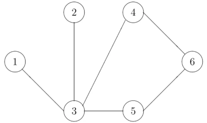
Smith (2002) addresses the transformation of (5) to a minimum cost flow problem. Define P_ρ as the set of all rings on which demand pair ρmay be satisfied, that is, forρ= (i, j)∈A, P_ρ = {k ∈ M : ˆx_ik = ˆx_jk = 1}. The minimum cost flow problem is then constructed with m+|A|+ 1 nodes. Nodes q_ρ correspond to each demand pair ρ∈ A and have a surplus of d^κ_ρ units, nodes t_k correspond to each ring k ∈ M and have a demand of b units, and node u is an intermediate node with a surplus/demand of mb−P

ρ∈Ad^κ_ρ units. For each ρ ∈ A, an arc with cost 0 exists from q_ρ to all nodes t_k such that k ∈ P_ρ. An arc also exists from

(12)

qρ to u with a cost of φρ for each ρ ∈ A. Finally, an arc with zero cost exists from u to nodet_k ∀k ∈M. Solving this network flow problem, we obtain the optimal f values on the arcs from the q nodes to the t nodes, and optimal w values on the arcs from the q nodes to node u. Consider the demand network depicted by Figure 1, and suppose that nodes 1, 2, 3, and 4 have been assigned to ring 1 and nodes 3, 4, 5, and 6 have been assigned to ring 2. The minimum cost flow network is shown in Figure 2, where the flow costs are displayed alongside the arcs and all demand and surplus values are displayed alongside their respective nodes.

¹¸

º·

¹¸

º·

¹¸

º·

¹¸

º·

¹¸

º·

¹¸

º·

@@

@

¢¢¢¢¢¢¢¢¢¢

¡¡¡¡¡

@@

@

4

6

5 1

2

3

Figure 1: Minimum Cost Flow Demand Graph.

The dual formulation to this network flow problem can be stated as follows, where dual variables α_ρ are associated with node q_ρ ∀ρ ∈ A, and variables β_k are associated with t_k ∀k ∈M. (The dual variable associated with u is arbitrarily set equal to 0.)

Maximize X

ρ∈A

d^κ_ρα_ρ−bX

k∈M

β_k (9a)

subject to

α_ρ−β_k ≤0 ∀ρ∈A, k ∈ P_ρ (9b)

α_ρ≤φ_ρ ∀ρ∈A (9c)

β_k≥0 ∀k∈M. (9d)

(13)

¹¸

º·

¹¸

º·

¹¸

º·

¹¸

º·

¹¸

º·

¹¸

º·

¹¸

º·

¹¸

º·

¹¸

º·

HHHH

HHHHH-Hj

³³³³³³³³³³1 HHHH

HHHH HHHj XXXXXXXXXXz

»»»»»»»»»»:

´´´´´´´´´´3

¡¡

¡¡ ª

´´

´´ +

»»

»» 9

XX XX XX XX X X y

QQ QQ QQ QQ QQ k

@@

@@ I

HHHH

HHHH HHHj

´´´´´´´´´´´3

u

q₁₃

q₂₃

q₃₄

q₄₆

q₅₆

q₃₅

t₁

t₂ 2b−P

ρ∈Ed^κ_ρ

d^κ₁₃ d^κ₂₃

d^κ₃₄

d^κ₄₆

d^κ₅₆

d^κ₃₅

−b

−b 0

0 0

0 0 0 0 φ₁₃

φ₂₃ φ₃₄ φ₄₆ φ56

φ₃₅ 0

0

Figure 2: Minimum Cost Flow Graph for the Demand Network Depicted in Figure 1.

It is not readily obvious how one can recover the optimalπ variables to (5), since primal constraints (4d) have been implicitly defined by the construction of the minimum cost flow problem. The following proposition prescribes a fast method for determining the optimal solution to (5) given an optimal dual basic feasible solution to (9).

Proposition 1. Given a binary network design vector ˆx and a corresponding optimal basic feasible solution (α^∗, β^∗) to (9), there exists an optimal solution to (5) in which λ^∗_ρ= dρα^∗_ρ ∀ρ∈A and µ^∗_k =β_k^∗ ∀k∈M. The optimal values for ¡

π^∗_ikρ, π_jkρ^∗ ¢

for ρ= (i, j)∈A are

(14)

determined as

¡π_ikρ^∗ , π_jkρ^∗ ¢

=











(0,0) if k∈ P_ρ orλ^∗_ρ≤d^κ_ρµ^∗_k (λ^∗_ρ−d^κ_ρµ^∗_k,0) if ˆx_ik = 0 and ˆx_jk = 1 (0, λ^∗_ρ−d^κ_ρµ^∗_k) if ˆx_jk = 1 and ˆx_jk = 0

Any solution toπ_ikρ^∗ +π_jkρ^∗ =λ^∗_ρ−d^κ_ρµ^∗_k, π_ikρ^∗ , π^∗_jkρ ≥0 if ˆx_ik = 0 and ˆx_jk = 0

(10)

Proof. Since models (5) and (9) are equivalent, we need to show that the objective function value given by (5a) for (λ^∗, µ^∗, π^∗) is the same as that given by (9a) for (α^∗, β^∗), and that (λ^∗, µ^∗, π^∗) is feasible to constraints (5b-d). The equivalence of the objective function values is clear, noting that

X

i∈N

X

k∈M

X

ρ∈Si

ˆ

x_ikπ_ikρ^∗ = 0

due to the construction of π^∗ values according to (10). For Constraints (5b) corresponding toρ∈Aandk ∈ Pρ, feasibility of (λ^∗, µ^∗, π^∗) is assured due to (9b). For (5b) corresponding to ρ= (i, j)∈A and k /∈ P_ρ, we must have by definition of P_ρ that at least one of ˆx_ik = 0 or ˆx_jk = 0. Hence, (π^∗_ikρ, π_jkρ^∗ ) is defined according to one of the latter three cases of (10) in order to ensure feasibility to (5b). Finally, Constraints (5c) and (5d) hold true due to (9c), (9d), and (10). This completes the proof. 2

The dual value recovery process reveals that when λ_ρ−d^κ_ρµ_k > 0 for some demand pair ρ = (i, j) ∈ A and k /∈ P_ρ such that ˆx_ik = ˆx_jk = 0, we must choose between setting π_ikρ or π_jkρ to equal this difference. The outcome of this decision has a direct impact on the optimality cut being passed back to the first-stage problem: if π_ikρ is set equal to λ_ρ−d^κ_ρµ_k, it will encourage nodeito be added to ringkin the next master problem iteration, and vice versa if π_jkρ is chosen to be positive. Magnanti and Wong (1981) underscore the

(15)

importance of properly selecting dual solutions by investigating methods by which dual solutions leading to nondominated Benders’ cuts may be identified. Unfortunately, each choice of dual values gives rise to a nondominated cut in the context of our problem. Since there are 2^h nondominated optimality cuts that can be formulated, whereh is the number of

“choices” as mentioned above, enumerating each possible cuts is computationally prohibitive.

We conducted a brief computational experiment to investigate the effectiveness of various rules for choosing among settingπikρ and πjkρ such thatπikρ+πjkρ =λρ−d^κ_ρµk. The results of this experiment indicate that setting either π_ikρ orπ_jkρ equal to λ_ρ−d^κ_ρµ_k when given a choice is the best strategy. We arbitrarily select π_ikρ=λ_ρ−d^κ_ρµ_k for the last case of (10) in our computational study in Section 5.

An alternative for resolving the choice in π-values is to consider the following problem reformulation. Define variable v_ρk = x_ikx_jk for ρ = (i, j)∈ A and k ∈ M. We may resolve this nonlinearity by enforcing the restrictions

v_ρk ≤x_ik, v_ρk ≤x_jk, and v_ρk ≥0 ∀ρ∈A, ∀k ∈M (11)

in (3) (and thus in (6) as well). Note that this technique is a subset of the linearization strategy employed in the Reformulation-Linearization Technique of Sherali and Adams (1990, 1994). We omit the lower bounding constraintv_ρk ≥x_ik+x_jk−1 since it will be implied at optimality. The second-stage problem may now be modified by replacing (4d) with

0≤f_ρk^κ ≤vρk ∀ρ∈A, ∀k ∈M, given scenario κ∈ {1, ..., r}. (12)

(16)

The dual problem would now be modified as follows, noting that only ˆv values need to be passed to the subproblem:

D(ˆv, ξ_κ) : MaximizeX

ρ∈A

λ_ρ−bX

k∈M

µ_k − X

ρ∈A

X

k∈M

ˆ

v_ρkπ_ρk (13a)

subject to

λρ−d^κ_ρµk−πρk ≤0 ∀k ∈M, ρ∈A (13b)

λ_ρ ≤d^κ_ρφ_ρ ∀ρ∈A (13c)

µ, π ≥0. (13d)

Using this higher-dimensional formulation, we would computeλand µvalues as before. The π values will now be set according to

πρk =









λ_ρ−d^κ_ρµ_k if λ_ρ−d^κ_ρµ_k >0

0 otherwise

∀ρ∈A, ∀k ∈M. (14)

Since no choice of optimality cuts are given, a unique dual solution exists to every nondegenerate primal problem. Moreover, it can be shown that this higher-dimensional representation captures all of the exponentially many cuts that may be identified from the original model.

The proof, omitted here for brevity, constructs any dual solution that could be obtained in the original model by surrogating (14) with negative multiples of the variable upper bounding constraints in (11).

3.3 Valid Inequality Generation

An important consideration in constructing a Benders-type decomposition algorithm with integer first-stage variables is the tightness of the master problem. If the master problem formulation is weak, excessive computational effort must be expended in finding an optimal solution to be passed to the second-stage subproblems. We thus develop classes of cutting

(17)

planes to reduce both the effort required to solve the master problem and the number of master problems that must be solved before the algorithm terminates.

Define a component G( ˆˆ N,A) ofˆ G(N, A) to be a connected subgraph such that if i ∈ Nˆ then neither edge (i, j) nor (j, i) belongs to A ∀j ∈ N \Nˆ, that is, ˆG is disconnected from the rest of the graph. We may then execute the following procedure, which enumerates all subsets of nodes in ˆN which may be placed on a ring, and evaluates whether the weighted amount of demand that could be satisfied on a ring containing these nodes would justify the requisite expenditure on ADM equipment.

Procedure 1. Consider the component ˆG( ˆN,A), and initially setˆ v = min(R,|Nˆ|).

Step 1. Ifv ≤1, go to Step 4. Else, select an ungenerated subset ˜N of ˆN such that|N˜|=v.

Create the graph ˜G( Ñ,A) by defining arc set ˜˜ A = {(i, j) ∈ Aˆ: i and j ∈N˜}, i.e., Ã is the set of arcs induced by Ñ on the graph ˆG. Set max_c = 0.

Step 2. For each scenarioξκ, κ= 1, ..., r, solve the linear knapsack problem c^κ = max X

ρ∈A˜

φ_ρd^κ_ρy_ρ (15a)

subject to X

ρ∈A˜

d^κ_ρy_ρ≤b (15b)

0≤yρ≤1 ∀ρ∈A,˜ (15c)

wherey_ρrepresents the fraction of demand satisfied for demand pairρ. IfP_r

κ=1p^κc^κ > max_c, setmax_c =P_r

κ=1p^κc^κ. If max_c> v, go to Step 3. Otherwise, if not all node subsets of size v have been generated, go to Step 1. Else set v =d(max_c−1)e and go to Step 1.

Step 3. Ifv < min{R,|Nˆ|}, generate the constraint P

i∈Nˆ x_ik ≤v ∀k ∈ M. In either case, terminate the procedure.

Step 4. Set x_ik = 0 ∀i∈N, kˆ ∈M and terminate.

(18)

The constraint generated in Step 3 is justified by observing that any solution containing a subgraph having at least v+ 1 of the nodes in ˆG on one of its rings may be improved or kept the same by removing those nodes from the ring. Hence, an optimal solution exists in which no ring contains v + 1 nodes of ˆG. The variable fixing in Step 4 is a special case of the constraint in Step 3 in which v = 0.

Unfortunately, the algorithm must enumerate a exponential number of subgraphs, and is not useful if R or |Nˆ| is large. We thus limit the use of this preprocessing algorithm to components having min(R,|Nˆ|) ≤ 4, ensuring the polynomiality of our preprocessing routine. (Note that Step 2 can be executed in O(r(n log n)) time, since we must solve r linear knapsack problems, each requiringO(n log n) computations.) A further rationale for limiting the size of subgraphs that may be enumerated is that the average number of arcs that exist in a subgraph grows quadratically in terms of the size of the subgraph. It thus becomes less likely to generate valid inequalities in Steps 3 or 4 as the size of the component increases.

Next, recall that no node will be assigned to a ring in an optimal solution unless an adjacent node in A is also assigned to the ring. (Otherwise, the node could be deleted without affecting the amount of demand that could be satisfied.) We thus incorporate the following connectivity constraints within the master problem.

x_ik ≤X

j∈Si

x_jk ∀i∈N, ∀k ∈M. (16)

Note that these constraints also implicitly require the valid restriction that each ring either contains zero or at least two ADMs.

Now, observe that since each SONET ring is identical, any given solution in which some ˆ

mrings are utilized to route demand has as many as ( ˆm!−1) alternatively optimal solutions

(19)

that may be obtained by simply reindexing the rings. Sherali and Smith (2000) and Sherali et al. (2000) have shown such symmetry unduly burdens a branch-and-bound approach to solving these problems by requiring the enumeration of several symmetrical branches. We state here two effective hierarchies for defeating this symmetry. The first requires that the number of nodes placed on ring k is no less than the number of nodes placed on ringk+ 1, for k = 1, ..., m−1, that is,

Xn

i=1

x_ik ≥ Xn

i=1

x_i,(k+1) ∀k = 1, ..., m−1. (17)

Note that although the hierarchy embodied by (17) is unlikely to completely break the symmetry within the model, it contains a constraint structure with nonzeros equal to 1 or - 1, which tends not to create additional fractional solutions in a branch-and-bound framework.

Alternatively, we may impose the following hierarchy, which requires that the sum of the node indices placed on ring k is no less than the sum of node indices placed on ring k+ 1, for k = 1, ..., m−1:

Xn

i=1

ix_ik ≥ Xn

i=1

ix_i,(k+1) ∀k = 1, ..., m−1. (18)

This hierarchy is more likely to eliminate all symmetric solutions, but is more likely to cause fractional solutions in addition to those that would normally be encountered in a branch- and-bound algorithm. Note that we may replace the sum of the indices in (18) with the sum squared of the indices, or any other reasonable exponent to further discourage symmetrical solutions, at the possible expense of creating additional fractional solutions.

3.4 Incorporating Subproblem Data Within the Master Problem

If demand shortage penalties are large relative to the cost of installing ADMs, several master problems must be solved before optimality cuts (8) relate ample information about demand shortage penalties under various proposed node to ring assignments. In this case, the fore-

(20)

going implementation of the decomposition algorithm will fail to converge in a reasonable amount of time. We offer a modification to the master problem that captures a minimum shortage penalty to be incurred for each demand pair given a proposed network design. First, let us define baseline demands, d, as follows.

d_ρ= min

κ∈{1,...,r}d^κ_ρ ∀ρ∈A.

Proposition 2. Given some binary vector x^∗, suppose (f^∗, w^∗) is an optimal solution to (3) with x ≡ x^∗ and demands given by d. Then for all demand pairs ρ ∈ A : w_ρ^∗ > 0, an optimal solution to each subproblem Q(x^∗, ξ_κ)∀κ = 1, ..., r exists in which the shortage for pair ρ is at least d_ρw_ρ^∗+¡

d^κ_ρ−d_ρ¢ .

Proof. We prove this proposition by induction, given any scenarioκ∈ {1, ..., r}and binary vectorx^∗. Recall from the discussion of Section 3.2 that given the node-to-ring assignments of a network, we may compute the optimal values for f and w by solving a minimum cost flow problem. This proposition trivially holds true ifd^κ =d. Now, suppose that the result is true for a set of demandsd, whered≤d≤d^κ, and define (f^∗, w^∗) to be the optimal solution to the minimum cost flow subproblem given x^∗ and d. Recall that the arcs corresponding to basic solution variables will form a tree with respect to the minimum cost flow graph.

Suppose that we seek a solution to the minimum cost flow problem in which the demands have changed to ˆd=d+e_ρ_ˆ, where e_ρ_ˆ is a vector of length |A| containing a 1 in the element corresponding to some ˆρ∈A and zeros elsewhere, for some ˆρ∈A such that d_ρ< d^κ_ρ. With respect to the minimum cost flow subproblem, this change is akin to increasing the surplus of q_ρ_ˆ by 1 and decreasing the surplus/demand of u by 1. Note that since the basic arcs of (f^∗, w^∗) form a tree, exactly one path (in the undirected sense) exists from q_ρ_ˆ to u. This path consists of a (possibly null) series of arcs between the q-nodes and t-nodes, followed

(21)

either by an arc from some q-node to u (call this a path of Type I), or an arc from some t-node to u (path of Type II).

Let us first consider the case in which all of the prior flow values along the arcs of the path from q_ρ_ˆ tou oriented in the opposite direction of the path are positive. We retain an optimal basic feasible solution with respect to demands ˆd by increasing the flows on arcs oriented in the same direction of the path by one, and decreasing the flows of arcs oriented in the opposite direction of the path by one. In particular, if w_ρ^∗_ˆ > 0, then an arc exists directly from q_ρ_ˆ tou, and flow is increased by one along this arc. However, if the path from q_ρ_ˆ to u is another path of Type I, the f-values in the new solution are modified, and the value of some otherw-variable increases by one. If a Type II path exists, we will modify the values of the f-variables, and will decrease the amount of unused capacity for some ring by decreasing the flow from node uto some t-node. In any of these cases, the previous solution continues to give rise to the same complementary slack primal and dual feasible bases. Since the w-values are nondecreasing, and sincew_ρ_ˆincreases by one if w^∗_ρ_ˆ was a positive value, we have that Proposition 2 holds true for this case.

We next discuss the case in which some arc oriented in the opposite direction of the path from q_ρ_ˆ to u has a flow of zero. Note that since w^∗_ρ_ˆ = 0 for this case, we must simply show that no w-values will decrease in the new solution. Suppose we follow the path from qρˆ to u, and identify the first degenerate basic arc oriented in the opposite direction of the path.

Removing this arc from the basis, we now have two components of the minimum cost flow graph with respect to the basic arcs. Note that the component containing node qρˆ does not contain node u, and thus a basic set of arcs is reconstituted by adding an arc from the component containingq_ρ_ˆto the component containingu. This connecting arc must either be

(22)

from aq-node to at-node, or from aq-node tou. A finite number of such degenerate pivots may need to be performed before a nondegenerate iteration takes place, at which time the situation reduces to the one addressed previously.

Note that we may iteratively construct any set of demands d^κ for κ ∈ {1, ..., r} by inde- pendently incrementing the baseline demands, with Proposition 2 holding true after each such incremental step. This completes the proof. 2

Suppose the deterministic ring design problem (1) is solved using the baseline demands, with one optimal solution having a set of shortages given by ˆw. The result of Proposition 2 implies that if ˆw_ρ >0 for some ρ ∈A, then there will exist an optimal recourse decision in which the shortage for demand pair ρ in scenario κ∈ {1, ..., r} is at least d_ρwˆ_ρ+¡

d^κ_ρ−d_ρ¢

units. The following baseline strategy explicitly solves the baseline demand problem in the first stage, and relates a minimum penalty measure that will be incurred in the second-stage problems to the first-stage variables. First, we include the following constraints within (6):

X

k∈M

f_ρk⁰ +w⁰_ρ= 1 ∀ρ∈A (19a)

X

ρ∈A

d_ρf_ρk⁰ ≤b ∀k ∈M (19b)

0≤f_ρk⁰ ≤xik ∀i∈N, ∀k ∈M, ∀ρ∈Si, and w⁰_ρ≥0 ∀ρ∈A. (19c)

To fully exploit the strength of Proposition 2, we introduce a new set of binary variables to the problem. Definey_ρ to equal 1 if a shortage for demand pair ρ∈A exists in the solution of the baseline demand, and 0 otherwise. We impose the following additional constraints in (6):

y_ρ ≥w_ρ⁰ and y_ρ ∈ {0,1} ∀ρ∈A (19d)

(23)

Θ_κ ≥X

ρ∈A

φ_ρ£ y_ρ¡

d^κ_ρ−d_ρ¢

+d_ρw⁰_ρ¤

∀κ= 1, ..., r. (19e)

Constraints (19d) state the lower bounds on the binary variables y, while constraints (19e) state the lower limits for shortage penalties given the baseline scenario solution. We will empirically examine the tradeoff between increasing the difficulty of the master problem by employing the baseline strategy embodied by (19) and the decrease in the number of problem iterations that must be executed.

4 Heuristic Procedure

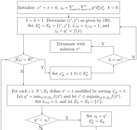
Since finding an optimal solution to Problem SRD may be too difficult to achieve within imposed computational limits, we may wish to quickly determine a heuristic solution to SRD. This solution would also benefit the multicut L-shaped algorithm of Section 3 by providing an upper bound to both the overall stochastic program and to each master integer program, and by prescribing a solution from which an initial set of optimality cuts may be obtained. We describe in this section the Greedy Augmenting Heuristic (GAH), which operates by selecting initial node-to-ring assignments for each ring, and then identifying promising augmentations of the proposed network design.

The logic of GAH is depicted as a flowchart in Figure 3. We first introduce a metric that measures the benefit of adding a node to a particular ring. Assume we are given a set of node-to-ring assignments previously prescribed by the heuristic. We define the utility of a nodeion a ringk as the additional amount of weighted demand that could be satisfied onk with the addition of nodei, minus the unit cost for including an extra ADM in the network.

GAH constructs one ring at a time by assigning to the ring currently under consideration a node having the highest utility, until the ring cardinality restriction is met.

(24)

Initialize: x^∗ = ˆx= 0, z₀ =P

ρ∈A

P_r

κ=1p^κd^κ_ρφ^κ_ρ, k = 0.

k =k+ 1. Determine (i^∗, j^∗) as given by (20).

Set E_k^∗ =Ek={i^∗, j^∗}, ˆxi^∗k = ˆxj^∗k = 1, and z_k =q^∗ =f(ˆx).

Terminate with solutionx^∗.

For each i∈N \E_k define ¯xⁱ = ˆx modified by setting ¯xⁱ_ik = 1.

Let q^∗ = min_i∈N\E_kf(¯xⁱ) and let i^∗ ∈argmin_i∈N\E_kf(¯xⁱ).

Set ˆx_i^∗_k= 1, and let E_k =E_k∪ {i^∗}.

Set x^∗_ik = 1 ∀i∈E_k^∗.

Set z_k =q^∗, E_k^∗ =Ek.

³³³³³ PPPPP

PP PP P

³³

³

|E_k|=R?

³³³³³ PPPPP

PP PP P

³³

³

q^∗ < z_k?

³³³³³ PPPPP

PP PP P

³³

³

k=m?

?

-

?

6

¾

?

- -

?

Y Y

Y

N

Figure 3: Heuristic Procedure for Generating Node-To-Ring Assignment.

We initialize the algorithm by setting the solution vector ˆx_ik = 0 ∀i∈N and k ∈M. For some assignment vectorx, definef(x) =P

i∈N

P

k∈M x_ik+Q(x), that is,f(x) is the optimal solution to SRD given x. We will denote by zk the best objective function value found after constructing (nonempty) rings 1, ..., k.

Given an empty ring currently under consideration, the utility of each node must equal zero. To prevent an arbitrary assignment of the initial node for an empty ring, we determine two initial nodes by identifying the “best” demand pair that could be added to a new ring.

Definexîj as ˆxmodified by setting ¯xîj_ik = ¯xîj_jk = 1, wherek is the new ring being constructed.

(25)

We initialize ring k with nodes i^∗ and j^∗ satisfying

ρ^∗ = (i^∗, j^∗)∈argmin_ρ∈A¡

f(x^ij)¢

. (20)

We may now meaningfully compute the utility of each node i∈N =N \ {i^∗, j^∗}. Let ¯xⁱ be the current vector, ˆx, modified by setting ¯xⁱ_ik = 1, i.e., adding nodei to the current ringk.

We compute the utility of node i on ring k as f(ˆx)−f(¯xⁱ), and identify the node with the best utility as

i^∗ ∈argmin_i∈N¡ f(xⁱ)¢

. (21)

Three properties of the behavior of GAH are discussed next that justify the remaining steps of the algorithm.

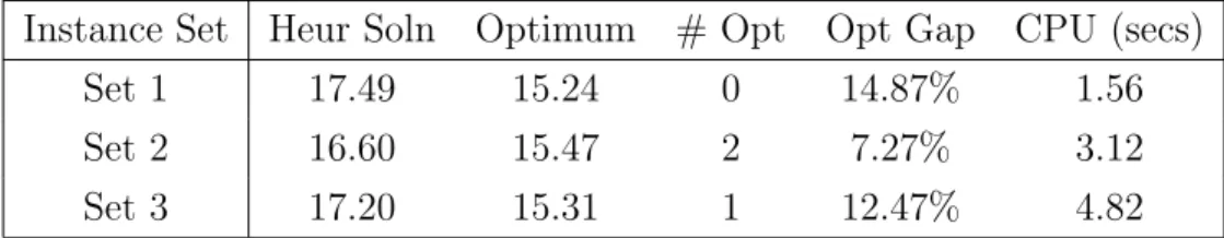
Property 1. Consider the construction of ring k by GAH, and let f(x^α_k) be the objective value obtained by the heuristic in constructing ringk, when ringk containedαnodes. Then f(x^α_k) is not necessarily quasiconvex in terms of α.

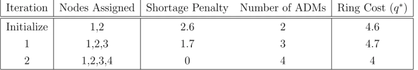
Example. Consider the demand graph given by Figure 4 as a one-scenario (deterministic) example whose penalties are given by the values alongside the arcs, and whose demands are given by d¹_ρ= 1 for all ρ ∈A. Suppose that the demand capacity restriction is set to b = 5 channels and that the node cardinality restriction is set to R = 4 nodes. Table 1 describes the construction of the first ring by GAH for this example. In this example, a two-node ring is more expensive than either a zero-node ring or a three-node ring. However, assigning all four nodes to the ring results in the least expensive design. 2

As a result of the foregoing property, GAH continues to add nodes to the current ring until the node cardinality limit is reached in hopes of identifying improved solutions. It is thus necessary to track the best objective value z_k achieved in the construction of the ring,

(26)

¹¸

º·

¹¸

º·

¹¸

º·

¹¸

º·

¡¡¡¡¡

¡¡

¡

@@

@

@@

@@@

0.4

2.0 0.9

0.9 1 0.4

2

3

4

Figure 4: Illustration of Property 1.

Iteration Nodes Assigned Shortage Penalty Number of ADMs Ring Cost (q^∗)

Initialize 1,2 2.6 2 4.6

1 1,2,3 1.7 3 4.7

2 1,2,3,4 0 4 4

Table 1: GAH Solution of Figure 4 Problem.

the set of nodes E_k^∗ assigned to ring k leading to that solution, and the current set of nodes E_k assigned to ring k. At the end of the construction of this ring, we set x^∗_ik = 1 ∀i∈E_k^∗.

Property 2 illustrates a similar behavior in the overall construction of the rings, wherein a ring may be constructed that temporarily worsens the objective function value, but ulti- mately leads to the construction of another ring that results in an improved solution.

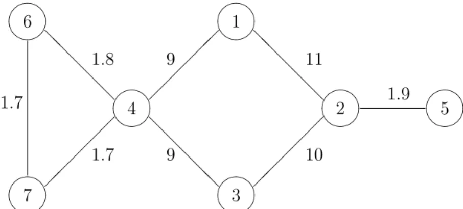
Property 2. The sequence of objective function valuesz_k, k= 1, ..., mis not quasiconvex in terms of k.

Example. We again consider a one-scenario instance whose demand network is depicted in Figure 5, where penalties are displayed alongside the arcs and d¹_ρ = 1 for all ρ ∈A, and instance parameters are defined as b = 6, R = 4, and m = 3. Table 2 summarizes the GAH steps for this example. Note that z₂ > z₁ and z₂ > z₃ for this example, justifying the construction of new rings even if previously constructed rings are not cost-efficient. 2