A computational study of a solver system forprocessing two-stage stochastic linearprogramming problems

(1)

A computational study of a solver system for processing two-stage stochastic linear

programming problems ^∗

Victor Zverovich

^†‡

Csaba I. F´ abi´ an

^§¶

Francis Ellison

^†‡

Gautam Mitra

^†‡

December 3, 2010

1 Introduction and background

Formulation of stochastic optimisation problems and computational algorithms for their solution continue to make steady progress as can be seen from an analysis of many developments in this field. The edited volume by Wallace and Ziemba (2005) outlines both the modelling systems for stochastic programming (SP) and many applications in diverse domains.

More recently, Fabozzi et al. (2007) have considered the application of SP models to challenging financial engineering problems. The tightly knit yet highly focused Stochastic Programming Community, their active website http://stoprog.org, and their triennial international SP conference points to the progressive acceptance of SP as a valuable decision tool. The Com- mittee on Stochastic Programming (COSP) exists as a standing committee of the Mathematical Optimization Society, and also serves as a liaison to related professional societies to promote stochastic programming.

At the same time many of the major software vendors, namely, XPRESS, AIMMS, MAXIMAL, and GAMS have started offering SP extensions to their

∗This is a revised version of the paper which appeared in SPEPS, Volume 2009, Nr. 3.

†CARISMA: The Centre for the Analysis of Risk and Optimisation Modelling Appli- cations, School of Information Systems, Computing and Mathematics, Brunel University, UK.

‡OptiRisk Systems, Uxbridge, Middlesex, UK.

§Institute of Informatics, Kecskemét College, 10 Izsáki út, Kecskemét, 6000, Hungary.

E-mail: fabian.csaba@gamf.kefo.hu.

¶Department of OR, Loránd Eötvös University, Budapest, Hungary.

(2)

optimisation suites.

Our analysis of the modelling and algorithmic solver requirements re- veals that (a) modelling support (b) scenario generation and (c) solution methods are three important aspects of a working SP system. Our research is focused on all three aspects and we refer the readers to Valente et al.

(2009) for modelling and Mitra et al. (2007) and Di Domenica et al. (2009) for scenario generation. In this paper we are concerned entirely with computational solution methods. Given the tremendous advances in LP solver algorithms there is a certain amount of complacency that by constructing a ”deterministic equivalent” problem it is possible to process most realistic instances of SP problems. In this paper we highlight the shortcoming of this line of argument. We describe the implementation and refinement of estab- lished algorithmic methods and report a computational study which clearly underpins the superior scale up properties of the solution methods which are described in this paper.

A taxonomy of the important class of SP problems may be found in Valente et al. (2008, 2009). The most important class of problems with many applications is the two-stage stochastic programming model with recourse;

this class of models originated from the early research of Dantzig (1955), Beale (1955) and Wets (1974).

A comprehensive treatment of the models and solution methods can be found in Kall and Wallace (1994), Pr´ekopa (1995), Birge and Louveaux (1997), Mayer (1998), Ruszczy´nski and Shapiro (2003), and Kall and Mayer (2005). Some of these monographs contain extensions of the original model.

Colombo et al. (2009) and Gassmann and Wallace (1996) describe computational studies which are based on interior point method and simplex based methods respectively. Birge (1997) covers a broad range of SP solution algorithms and applications in his survey.

The rest of this paper is organised in the following way. In section 2 we introduce the model setting of the two stage stochastic programming problem, in section 3 we consider a selection of solution methods for processing this class of problems. First we consider direct solution of the deterministic equivalent LP problem. Then we discuss Benders decomposition, and the need for regularisation. We first present the Regularized Decomposition method of Ruszczy´nski (1986) and then introduce another regularisation approach in some detail, namely, the Level Method (Lemar´echal et al., 1995) adapted for the two-stage stochastic programming problem. Finally we outline the box-constrained trust-region method of Linderoth and Wright (2003).

In section 4 we discuss implementation issues, in section 5 we set out the computational study and in section 6 we summarise our conclusions.

(3)

2 The model setting

2.1 Two-stage problems

In this paper we only consider linear SP models and assume that the random parameters have a discrete finite distribution. This class is based on two key concepts of (i) a finite set of discrete scenarios (of model parameters) and (ii) a partition of variables to first stage (”here and now”) decision variables and a second stage observation of the parameter realisations and corrective actions and the corresponding recourse (decision) variables.

The first stage decisions are represented by the vector x. Assume there are S possible outcomes (scenarios) of the random event, the ith outcome occurring with probabilityp_i. Suppose the first stage decision has been made with the resultx, and theith scenario is realised. The second stage decisiony is computed by solving the followingsecond-stage problemorrecourse problem

R_i(x) : min q^T_i y

subject to T_ix+W_iy =h_i, y≥0,

(1) where q_i, h_i are given vectors andT_i, W_i are given matrices. LetK_i denote the set of thosexvectors for which the recourse problemR_i(x) has a feasible solution. This is a convex polyhedron. For x ∈ K_i, let q_i(x) denote the optimal objective value of the recourse problem. We assume that q_i(x) >

−∞. (Or equivalently, we assume that the dual of the recourse problemR_i(x) has a feasible solution. Solvability of the dual problem does not depend on x.) The function q_i : K_i → IR is apolyhedral (i.e., piecewise linear) convex function.

The customary formulation of thefirst-stage problem is stated as:

min c^Tx+

S

P

i=1

p_iq_i(x) subject to x∈X,

x∈K_i (i= 1, . . . , S),

(2)

where X := {x|Ax=b, x≥0} is a non-empty bounded polyhedron de- scribing the constraints, c and b are given vectors and A is a given matrix, with compatible sizes. The objective, F(x) :=

S

P

i=1

p_iq_i(x), is defined as an expected value and is called the expected recourse function. This is a polyhedral convex function with the domain K :=K₁∩. . .∩K_S.

This two-stage stochastic programming problem ((2) and (1)) can be formulated as a single linear programming problem called the deterministic

(4)

equivalent problem:

min c^Tx + p₁q₁^Ty₁ + . . . + p_Sq_S^Ty_S

subject to Ax = b,

T₁x + W₁y₁ = h₁,

... . .. ...

T_Sx + W_Sy_S = h_S,

x≥0,y1 ≥0, . . . , yS ≥0.

(3)

3 A selection of methods

3.1 Solution of the deterministic equivalent problem

The deterministic equivalent problem (3) can be solved as a linear programming problem, either by the simplex method or by an interior-point method.

In this computational study we use general-purpose LP solvers for the solution of the deterministic equivalent problem.

3.2 Decomposition methods

The deterministic equivalent problem (3) is a linear programming problem of a specific structure: for each scenario, a subproblem is included that de- scribes the second-stage decision associated with the corresponding scenario realisation. The subproblems are linked by the first-stage decision variables.

Dantzig and Madansky (1961) observed that the dual of the deterministic equivalent problem fits the prototype for the Dantzig-Wolfe decomposition (1960).

Van Slyke and Wets (1969) proposed a cutting-plane approach for the first-stage problem (2). Their L-Shaped method builds respective cutting- plane models of the feasible domain K =K₁∩. . .∩K_S and of the expected recourse function F =

S

P

i=1

p_iq_i. We outline cutting-plane models and their relationship with decomposition.

Let us denote the dual ofR_i(x) in (1) as

Di(x) : max z^T(hi−Tix)

subject to W_i^Tz ≤q_i, (4) where z is a real-valued vector.

The feasible region is a convex polyhedron that we assumed nonempty.

We will characterise this polyhedron by two finite sets of vectors: letU_iandV_i

(5)

denote the sets of the extremal points and of the extremal rays, respectively, in case the polyhedron can be represented by these sets. To handle the general case, we require further formalism; let us add a slack vectorγ of appropriate dimension, and use the notation [W_i^T, I](z,γ) =W_i^Tz+γ. Given a composite vector (z,γ) of appropriate dimensions, let support(z,γ) denote the set of those column-vectors of the composite matrix [W_i^T, I] that belong to non-zero (z,γ)-components. Using these, let

U_i:=

z

W_i^Tz+γ =q_i,γ ≥0, support(z,γ) is a linearly independent set , Vi:=

z

W_i^Tz+γ =0,γ≥0, support(z,γ) is a minimal dependent set . These are finite sets, and the feasible domain of the dual problem D_i(x) in (4) can be represented as convex combinations of Ui-elements added to cone-combinations of V_i-elements.

We have x ∈ K_i if and only if the dual problem D_i(x) has a finite optimum, that is,

v_i^T(h_i−T_ix)≤0 holds for everyv_i ∈V_i.

In this case, the optimum of D_i(x) is attained at an extremal point, and can be computed as

min ϑi

subject to ϑ_i ∈IR,

u^T_i (h_i−T_ix)≤ϑ_i (u_i ∈U_i).

By the linear programming duality theorem, the optimum of the above problem is equal to q_i(x); hence the first-stage problem (2) is written as

min c^Tx+

S

P

i=1

p_iϑ_i

subject to x∈X, ϑ_i ∈IR (i= 1, . . . , S),

v^T_i (h_i−T_ix)≤0 (v_i∈V_i, i= 1, . . . , S), u^T_i (hi−Tix)≤ϑi (ui∈Ui, i= 1, . . . , S);

(5)

This we call the disaggregated form. The aggregated form is stated as min c^Tx+ϑ

subject to x∈X, ϑ ∈IR,

v_i^T(h_i−T_ix)≤0 (v_i∈V_i, i= 1, . . . , S),

S

P

i=1

p_iu^T_i (h_i−T_ix)≤ϑ (u₁, . . . ,u_S)∈ U ,

(6)

where U ⊂U₁× · · · ×U_S is a subset that contains an element for each facet in the graph of the polyhedral convex function F; formally, we have

F(x) =

S

X

i=1

p_i max u_i∈Ui

u^T_i (h_i−T_ix)

= max

(u₁,...,u_s)∈U S

X

i=1

p_iu^T_i (h_i−T_ix).

Cutting-plane methods can be devised on the basis of either the disaggregated formulation (5) or the aggregated formulation (6). These are processed by iterative methods that build respective cutting-plane models of the feasible setK and the expected recourse functionF. The cuts belonging to the model of K are called feasibility cuts, and those belonging to the model of F are calledoptimality cuts. Cuts at a given iteratexb are generated by solving the dual problems D_i(x) (ib = 1, . . . , S). Problems with unbounded objectives yield feasibility cuts, and problems with optimal solutions yield optimality cuts.

In its original form, the L-Shaped method of Van Slyke and Wets (1969) works on the aggregated problem. A multicut version that works on the disaggregated problem was proposed by Birge and Louveaux (1988).

There is a close relationship between decomposition and cutting-plane approaches. It turns out that the following approaches yield methods that are in principle identical:

– cutting-plane method for either the disaggregated problem (5) or the aggregated problem (6),

– Dantzig-Wolfe decomposition (1960) applied to the dual of the deterministic equivalent problem (3),

– Benders decomposition (1962) applied to the deterministic equivalent problem (3).

Cutting-plane formulations have the advantage that they give a clear visual illustration of the procedure. A state-of-the-art overview of decomposition methods can be found in Ruszczy´nski (2003).

Aggregated vs disaggregated formulations

The difference between the aggregated and the disaggregated problem formulations may result in a substantial difference in the efficiency of the solution methods. By using disaggregated cuts, more detailed information is stored in the master problem, hence the number of the master iterations is reduced in general. This is done at the expense of larger master problems.

(7)

Based on the numerical results of Birge and Louveaux (1988) and Gassmann (1990), Birge and Louveaux (1997) conclude that the multicut approach is in general more effective when the number of the scenarios is not significantly larger than the number of the constraints in the first-stage problem.

3.3 Regularisation and trust region methods

It is observed that successive iterations do not generally produce an orderly progression of solutions - in the sense that while the change in objective value from one iteration to the next may be very small, even zero, a wide difference may exist between corresponding values of the first-stage variables.

This feature of zigzagging in cutting plane methods is the consequence of using a linear approximation. Improved methods were developed that use quadratic approximation: proximal point method by Rockafellar (1976), and bundle methods by Lemar´echal (1978) and Kiwiel (1985). These methods construct a sequence of stability centers together with the sequence of the iterates. When computing the next iterate, roaming away from the current stability center is penalised.

Another approach is the trust region methods, where a trust region is constructed around the current stability center, and the next iterate is selected from this trust region.

Regularized decomposition

The Regularized Decomposition (RD) method of Ruszczy´nski (1986) is a bundle-type method applied to the minimisation of the sum of polyhedral convex functions over a convex polyhedron, hence this method fits the disaggregated problem (5). The RD method lays an emphasis on keeping the master problem as small as possible. (This is achieved by an effective constraint reduction strategy.) A recent discussion of the RD method can be found in Ruszczy´nski (2003).

Ruszczy´nski and ´Swi¸etanowski (1997) implemented the RD method, and solved two-stage stochastic programming problems, with a growing scenario set. Their test results show that the RD method is capable of handling large problems.

The level method

A more recent development in convex programming is the level method of Lemar´echal, Nemirovskii, and Nesterov (1995). This is a special bundle-type method that uses level sets of the model functions for regularisation. Let us

(8)

consider the problem

min f(x) subject to x∈X,

(7) where X ⊂IRⁿ is a convex bounded polyhedron, and f a real-valued convex function, Lipschitzian relative toX. The level method is an iterative method, a direct generalization of the classical cutting-plane method. Acutting-plane model of f is maintained using function values and subgradients computed at the known iterates. Let f denote the current model function; this is the upper cover of the linear support functions drawn at the known iterates.

Hence f is a polyhedral convex lower approximation of f. The level sets of the model function are used for regularization.

Let ˆx denote the current iterate. Let F^? denote the minimum of the objective values in the known iterates. Obviously F^? is an upper bound for the optimum of (7).

Let F := min

x∈Xf(x) denote the minimum of the current model function over the feasible polyhedron. Obviously F is a lower bound for the optimum of (7).

If the gap F^? −F is small, then the algorithm stops. Otherwise let us consider the level set of the current model function belonging to the level (1−λ)F^?+λF where 0< λ < 1 is a fixed parameter. Using formulas, the current level set is

Xˆ :=

x∈X

f(x)≤(1−λ)F^?+λF .

The next iterate is obtained byprojectingthe current iterate onto the current level set. Formally, the next iterate is an optimal solution of the convex quadratic programming problem minkx−xkˆ ² subject tox∈X.ˆ

Lemar´echal et al. (1995) gives the following efficiency estimate: To obtain a gap smaller than , it suffices to perform

κ DL

2

(8) iterations, whereDis the diameter of the feasible polyhedron,Lis a Lipschitz constant of the objective function, and κis a constant that depends only on the parameter of the algorithm.

Remark 1 The method in general performs much better than the estimate (8) implies: F´abi´an and Sz˝oke (2007) solved problems with different settings of the stopping tolerance , and the number of the required iterations was found to be proportional to log(1/).

(9)

The estimate (8) generally yields bounds too large for practical purposes.

We include this estimate because it is essentially different from the classic finiteness results obtained when a polyhedral convex function is minimised by a cutting-plane method. Finiteness results are based on enumeration. The straightforward finiteness proof assumes that basic solutions are found for the model problems, and that there is no degeneracy. An interesting finiteness proof that allows for nonbasic solutions is presented in Ruszczy´nski (2006).

This is based on the enumeration of the cells (i.e., polyhedrons, facets, edges, vertices) that the linear pieces of the objective function define.

Remark 2 The level method can be implemented for the case when the feasible domain X is not bounded. The theoretical estimate given in (8) is not applicable in this case, but the method works. Finiteness can be proven by applying the arguments set out in remark 1, above.

F´abi´an and Sz˝oke (2007) adapted the level method to the solution of two- stage stochastic programming problems, and solved two-stage stochastic programming problems with growing scenario sets. According to the results presented, there is no correlation between the number of the scenarios and the number of the master iterations required (provided that the number of the scenarios is large enough).

Remark 3 The Level Decomposition (LD) method proposed in Fábián and Sz˝oke (2007) handles feasibility and optimality issues simultaneously, in a unified manner. Moreover the LD framework allows a progressive approximation of the distribution, and approximate solution of the second-stage problems. – This is facilitated by an inexact version Fábián (2000) of the level method. The inexact method uses approximate data to construct a model of the objective function. At the beginning of the procedure, a rough approximation is used, and the accuracy is gradually increased as the optimum is approached. – Numerical results of Fábián and Sz˝oke (2007) show that this progressive approximation framework is effective: although the number of the master iterations is larger than in the case of the exact method, there is a substantial reduction in solution time of the second-stage problems.

In this study we use the original (exact) level method hence no progressive approximation is performed. Moreover, only the objective function is regularised, as in the classical regularisation approaches. That is why regularisation does not extend to feasibility issues.

Box-constrained method

The box-constrained trust-region method of Linderoth and Wright (2003) solves the disaggregated problem (5), and uses a special trust-region ap-

(10)

proach.

Trust-region methods construct a sequence of stability centers together with the sequence of the iterates. Trust regions are constructed around the stability centers, and the next iterate is selected from the current trust region.

Linderoth and Wright construct box-shaped trust regions, hence the resulting master problems remain linear. The size of the trust region is continually adapted on the basis of the quality of the current solution.

4 Algorithmic descriptions and implementa- tion issues

All solution methods considered in the current study were implemented within the FortSP stochastic solver system (Ellison et al., 2010) which in- cludes an extensible algorithmic framework for creating decomposition-based methods. The following algorithms were implemented based on this framework:

• Benders decomposition (Benders),

• Benders decomposition with regularisation by the level method (Level),

• the trust region method based on l∞ norm (TR),

• regularized decomposition (RD).

For more details including the solver system architecture and pseudo- code of each method refer to Ellison et al. Here we present only the most important details specific to our implementation.

4.1 Solution of the deterministic equivalent by simplex and interior-point methods

The first approach to solve stochastic linear programming problems we considered was using a state-of-the-art LP solver to optimise the deterministic equivalent problem (3). For this purpose CPLEX barrier and dual simplex optimisers were selected since they provide high-performance implementation of corresponding methods.

We also solved our problems by the HOPDM solver (Gondzio, 1995;

Colombo and Gondzio, 2008), an implementation of the infeasible primal- dual interior point method.

(11)

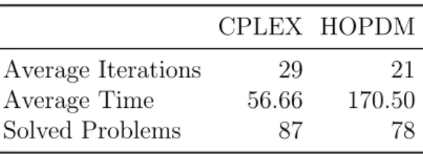
Table 1: Summary of CPLEX and HOPDM performance CPLEX HOPDM

Average Iterations 29 21

Average Time 56.66 170.50

Solved Problems 87 78

The results summarised in Table 1 show that while it took HOPDM on average less iterations to solve a problem, CPLEX was faster in our bench- marks. This can be explained by the latter being better optimised to the underlying hardware. In particular, CPLEX uses high performance Intel Math Kernel Library which is tuned for the hardware we were using in the tests.

4.2 Benders decomposition

For the present computational study, we have implemented a decomposition method that works on the aggregated problem (6). After a certain number of iterations, let Vb_i ⊂V_i denote the subsets of the known elements ofV_i (i= 1, . . . , S), respectively. Similarly, let U ⊂ Ub denote the subset of the known elements of U ⊂U₁× · · · ×U_S. We solve the current problem

min c^Tx+ϑ

subject to x∈X, ϑ ∈IR,

v_i^T(h_i−T_ix)≤0 (v_i∈Vb_i, i= 1, . . . , S),

S

P

i=1

p_iu^T_i (h_i−T_ix)≤ϑ (u₁, . . . ,u_S)∈Ub .

(9)

If the problem (9) is infeasible, then so is the original problem. Letxb denote an optimal solution. In order to generate cuts atx, we solve the dual recourseb problems D_i(x) (ib = 1, . . . , S) with a simplex-type method. Let

Ib:={1≤i≤S|problem D_i(x) has unbounded objective}b .

If Ib=∅ then the solution process of each dual recourse problem terminated with an optimal basic solution ub_i ∈U_i. If xb is near-optimal then the procedure stops. Otherwise we add the point (ub₁, . . . ,ub_S) toUb, rebuild the model problem (9), and start a new iteration.

If Ib6= ∅ then for i ∈ I, the solution process of the dual recourse prob-b lem D_i(x) terminated withb vb_i ∈ V_i. We add vb_i to Vb_i (i ∈ Ib), rebuild the problem (9), and start a new iteration.

(12)

4.3 Benders decomposition with level regularisation

On the basis of the decomposition method described above we implemented a rudimentary version of the level decomposition. We use the original exact level method, hence we use no distribution approximation, and second-stage problems are solved exactly (i.e., with the same high accuracy always). Al- gorithm 1 shows the pseudo-code for the method.

Our computational results reported in section 5.3 show that level-type regularisation is indeed advantageous.

4.4 Regularized decomposition

In addition to the methods that work on the aggregated problem we implemented two algorithms based on the disaggregated (multicut) formulation (5).

The first method is Regularized Decomposition (RD) of Ruszczy´nski (1986). For this method we implemented deletion of inactive cuts and the rules for dynamic adaptation of the penalty parameter σ as described by Ruszczy´nski and ´Swi¸etanowski (1997):

• if F(x^k)> γF(¯x^k) + (1−γ) ˆF^k then σ ←σ/2,

• if F(x^k)<(1−γ)F(¯x^k) +γFˆ^k then σ ←2σ,

wherex¯^k is a reference point, (x^k,ϑ^k) is a solution of the master problem at the iteration k, ˆF^k = c^Tx^k +

S

P

i=1

p_iϑ^k_i, F(x) = c^Tx +

S

P

i=1

p_iq_i(x) and γ ∈(0,1) is a parameter.

Regularised master problem at the iterationk is formulated as follows:

min c^Tx+

S

P

i=1

piϑi+_2σ¹ kx−x¯^kk²

subject to x∈X, ϑ_i ∈IR (i= 1, . . . , S),

v^T_i (h_i−T_ix)≤0 (v_i ∈Vb_i, i= 1, . . . , S), u^T_i (h_i−T_ix)≤ϑ_i (u_i ∈Ub_i, i= 1, . . . , S).

(10)

For a more detailed description of the implementation including the pseudo- code please refer to Ellison et al. (2010).

4.5 The trust region method based on the infinity norm

We also implemented the l∞ trust region L-shaped method of Linderoth and Wright (2003). It operates on the disaggregated problem (5) with additional

(13)

Algorithm 1Benders decomposition with regularisation by the level method choose iteration limit k_max ∈Z⁺

choose relative stopping tolerance ∈R+

solve the expected value problem to get a solution x⁰ (initial iterate) k ←0,F^∗ ← ∞

choose λ∈(0,1) F⁰ ← −∞

while time limit is not reached and k < k_max do

solve the recourse problems (1) with x=x^k and compute F(x^k) if all recourse problems are feasible then

add an optimality cut if F(x^k)< F^∗ then

F^∗ ←F(x^k) x^∗ ←x^k end if else

add a feasibility cut end if

if (F^∗−F^k)/(|F^∗|+ 10⁻¹⁰)≤ then stop

end if

solve the master problem (9) to get an optimal solution (x⁰,ϑ⁰) and the optimal objective value F^k+1.

if (F^∗−F^k+1)/(|F^∗|+ 10⁻¹⁰)≤ then stop

end if

solve the projection problem:

min kx−x⁰k²

subject to c^Tx+ϑ≤(1−λ)F^k+1+λF^∗ x∈X, ϑ ∈IR,

v_i^T(hi−Tix)≤0 (vi ∈Vbi, i= 1, . . . , S),

S

P

i=1

p_iu^T_i (h_i−T_ix)≤ϑ (u₁, . . . ,u_S)∈Ub .

let (x^k+1,θ^k+1) be an optimal solution of the projection problem; then x^k+1 is the next iterate

k ←k+ 1 end while

Here ˆF^k=c^Tx^k+ϑ^k and F(x) =c^Tx+

S

P

i=1

p_iq_i(x).

(14)

bounds of the form

−∆e≤x−x¯^k≤∆e, (11) where ∆ is the trust region radius, e= (1,1, . . . ,1) and x¯^k is a reference point at the iterationk. The rules of updating ∆ are the same as in Linderoth and Wright (2003) and are outlined below (counter is initially set to 0):

if F(¯x^k)−F(x^k)≥ξ(F(x¯^k)−Fˆ^k) then

if F(¯x^k)−F(x^k)≥0.5(F(¯x^k)−Fˆ^k) and k¯x^k−x^kk∞= ∆ then

∆←min(2∆,∆hi) end if

counter ←0 else

ρ← −min(1,∆)(F(¯x^k)−F(x^k))/(F(x¯^k)−Fˆ^k) if ρ >0then

counter ← counter + 1 end if

if ρ >3or (counter ≥3 and ρ∈(1,3]) then

∆←∆/min(ρ,4) counter ← 0 end if

end if

Fˆ^k =c^Tx^k+

S

P

i=1

piϑ^k_i, where (x^k,ϑ^k) is a solution of the master problem at the iteration k, ∆_hi is an upper bound on the radius and ξ∈(0,1/2) is a parameter. The complete pseudo-code of the method can be found in Ellison et al. (2010).

5 Computational study

5.1 Experimental setup

The computational experiments were performed on a Linux machine with 2.4 GHz Intel CORE i5 M520 CPU and 6 GiB of RAM. Deterministic equivalents were solved with CPLEX 12.1 dual simplex and barrier optimisers. Crossover to a basic solution was disabled for the barrier optimiser and the number of threads was limited to 1. For other CPLEX options the default values were used.

The times are reported in seconds with times of reading input files not included. For simplex and IPM the times of constructing deterministic equivalent problems are included though it should be noted that they only amount to small fractions of the total. CPLEX linear and quadratic programming

(15)

Table 2: Sources of test problems

Source Reference Comments

1. POSTS collection

Holmes (1995) Two-stage problems from the (PO)rtable (S)tochastic programming (T)est (S)et (POSTS) 2. Slptestset

collection

Ariyawansa and Felt (2004)

Two-stage problems from the collection of stochastic LP test problems

3. Random problems

Kall and Mayer (1998)

Artificial test problems generated with pseudo random stochastic LP problem generator GENSLP 4. SAMPL

problems

K¨onig et al. (2007), Valente et al. (2008)

Problems instantiated from the SAPHIR gas portfolio planning model formulated in Stochastic AMPL (SAMPL)

solver was used to solve master problem and subproblems in the decomposition methods. All the test problems were presented in SMPS format introduced by Birge et al. (1987).

The first-stage solution of the expected value problem was taken as a starting point for the decomposition methods. The values of the parameters are specified below.

• Benders decomposition with regularisation by the level method:

λ= 0.5,

• Regularized decomposition:

σ = 1, γ = 0.9.

• Trust region method based on l∞ norm:

∆ = 1,∆_hi = 10³ (except for the saphir problems where ∆_hi = 10⁹), ξ = 10⁻⁴.

5.2 Data sets

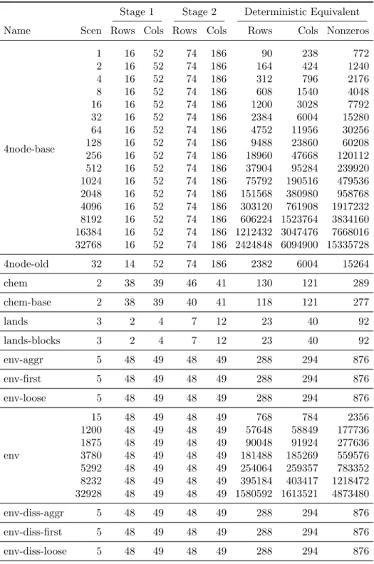
We considered test problems which were drawn from four different sources described in Table 2. Table 3 gives the dimensions of these problems.

Most of the benchmark problems have stochasticity only in the right-hand side (RHS). Notable exception is the SAPHIR family of problems which has random elements both in the RHS and the constraint matrix.

(16)

Table 3: Dimensions of test problems

Stage 1 Stage 2 Deterministic Equivalent Name Scen Rows Cols Rows Cols Rows Cols Nonzeros

fxm 6 92 114 238 343 1520 2172 12139

16 92 114 238 343 3900 5602 31239

fxmev 1 92 114 238 343 330 457 2589

pltexpa 6 62 188 104 272 686 1820 3703

16 62 188 104 272 1726 4540 9233

stormg2

8 185 121 528 1259 4409 10193 27424 27 185 121 528 1259 14441 34114 90903 125 185 121 528 1259 66185 157496 418321 1000 185 121 528 1259 528185 1259121 3341696

airl-first 25 2 4 6 8 152 204 604

airl-second 25 2 4 6 8 152 204 604

airl-randgen 676 2 4 6 8 4058 5412 16228

assets 100 5 13 5 13 505 1313 2621

37500 5 13 5 13 187505 487513 975021

4node

1 14 52 74 186 88 238 756

2 14 52 74 186 162 424 1224

4 14 52 74 186 310 796 2160

8 14 52 74 186 606 1540 4032

16 14 52 74 186 1198 3028 7776

32 14 52 74 186 2382 6004 15264

64 14 52 74 186 4750 11956 30240

128 14 52 74 186 9486 23860 60192

256 14 52 74 186 18958 47668 120096

512 14 52 74 186 37902 95284 239904

1024 14 52 74 186 75790 190516 479520 2048 14 52 74 186 151566 380980 958752 4096 14 52 74 186 303118 761908 1917216 8192 14 52 74 186 606222 1523764 3834144 16384 14 52 74 186 1212430 3047476 7668000 32768 14 52 74 186 2424846 6094900 15335712

(17)

Table 3: Dimensions of test problems (continued)

4node-base

1 16 52 74 186 90 238 772

2 16 52 74 186 164 424 1240

4 16 52 74 186 312 796 2176

8 16 52 74 186 608 1540 4048

16 16 52 74 186 1200 3028 7792

32 16 52 74 186 2384 6004 15280

64 16 52 74 186 4752 11956 30256

128 16 52 74 186 9488 23860 60208

256 16 52 74 186 18960 47668 120112

512 16 52 74 186 37904 95284 239920

1024 16 52 74 186 75792 190516 479536 2048 16 52 74 186 151568 380980 958768 4096 16 52 74 186 303120 761908 1917232 8192 16 52 74 186 606224 1523764 3834160 16384 16 52 74 186 1212432 3047476 7668016 32768 16 52 74 186 2424848 6094900 15335728

4node-old 32 14 52 74 186 2382 6004 15264

chem 2 38 39 46 41 130 121 289

chem-base 2 38 39 40 41 118 121 277

lands 3 2 4 7 12 23 40 92

lands-blocks 3 2 4 7 12 23 40 92

env-aggr 5 48 49 48 49 288 294 876

env-first 5 48 49 48 49 288 294 876

env-loose 5 48 49 48 49 288 294 876

env

15 48 49 48 49 768 784 2356

1200 48 49 48 49 57648 58849 177736

1875 48 49 48 49 90048 91924 277636

3780 48 49 48 49 181488 185269 559576 5292 48 49 48 49 254064 259357 783352 8232 48 49 48 49 395184 403417 1218472 32928 48 49 48 49 1580592 1613521 4873480

env-diss-aggr 5 48 49 48 49 288 294 876

env-diss-first 5 48 49 48 49 288 294 876

env-diss-loose 5 48 49 48 49 288 294 876

(18)

Table 3: Dimensions of test problems (continued)

env-diss

15 48 49 48 49 768 784 2356

1200 48 49 48 49 57648 58849 177736

1875 48 49 48 49 90048 91924 277636

3780 48 49 48 49 181488 185269 559576 5292 48 49 48 49 254064 259357 783352 8232 48 49 48 49 395184 403417 1218472 32928 48 49 48 49 1580592 1613521 4873480

phone1 1 1 8 23 85 24 93 309

phone 32768 1 8 23 85 753665 2785288 9863176

stocfor1 1 15 15 102 96 117 111 447

stocfor2 64 15 15 102 96 6543 6159 26907

rand0

2000 50 100 25 50 50050 100100 754501 4000 50 100 25 50 100050 200100 1508501 6000 50 100 25 50 150050 300100 2262501 8000 50 100 25 50 200050 400100 3016501 10000 50 100 25 50 250050 500100 3770501

rand1

2000 100 200 50 100 100100 200200 3006001 4000 100 200 50 100 200100 400200 6010001 6000 100 200 50 100 300100 600200 9014001 8000 100 200 50 100 400100 800200 12018001 10000 100 200 50 100 500100 1000200 15022001

rand2

2000 150 300 75 150 150150 300300 6758501 4000 150 300 75 150 300150 600300 13512501 6000 150 300 75 150 450150 900300 20266501 8000 150 300 75 150 600150 1200300 27020501 10000 150 300 75 150 750150 1500300 33774501

saphir

50 32 53 8678 3924 433932 196253 1136753 100 32 53 8678 3924 867832 392453 2273403 200 32 53 8678 3924 1735632 784853 4546703 500 32 53 8678 3924 4339032 1962053 11366603 1000 32 53 8678 3924 8678032 3924053 22733103

It should be noted that the problems generated with GENSLP do not pos- sess any internal structure inherent in real-world problems. However they are still useful for the purposes of comparing scale-up properties of algorithms.

(19)

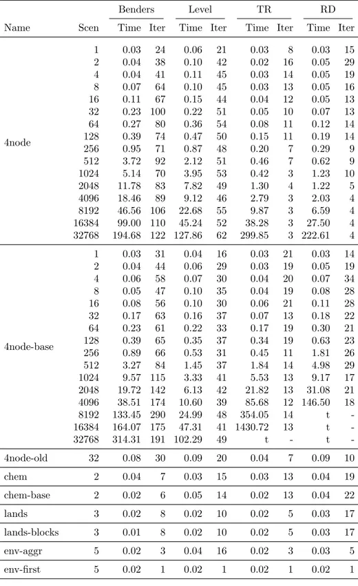
5.3 Computational results

The computational results are presented in Tables 4 and 5. Iter denotes the number of iterations. For decomposition methods this is the number of master iterations.

We refer to the methods using the following abbreviations:

Abbreviation Full name Reference

DEP-Simplex Simplex method applied to the deterministic equivalent problem (DEP)

Section 4.1 DEP-IPM Interior point method applied to the DEP Section 4.1

Benders Benders decomposition Section 4.2

Level Benders decomposition with level regularisation

Section 4.3

RD Regularized decomposition Section 4.4

TR Trust region method Section 4.5

Finally we present the results in the form of performance profiles. The performance profile for a solver is defined by Dolan and Mor´e (2002) as the cumulative distribution function for a performance metric. We use the ratio of the solving time versus the best time as the performance metric. Let P and M be the set of problems and the set of solution methods respectively.

We define by t_p,m the time of solving problem p ∈ P with method m ∈M. For every pair (p, m) we compute performance ratio

r_p,m = t_p,m

min{t_p,m|m ∈M},

If method m failed to solve problem p the formula above is not defined.

In this case we set r_p,m :=∞.

The cumulative distribution function for the performance ratio is defined as follows:

ρm(τ) = |{p∈P|r_p,m ≤τ}|

|P|

We calculated performance profile of each considered method on the whole set of test problems. These profiles are shown in Figure 1. The value of ρ_m(τ) gives the probability that methodm solves a problem within a ratio τ of the best solver. For example according to Figure 1 the level method was the first in 25% of cases and solved 95% of the problems within a ratio 11 of the best time.

The notable advantages of performance profiles over other approaches to performance comparison are as follows. Firstly, they minimize the influence

(20)

of a small subset of problems on the benchmarking process. Secondly, there is no need to discard solver failures. Thirdly, performance profiles provide a visualisation of large sets of test results as we have in our case. It should be noted, however, that we still investigated the failures and the cases of unusual performance. This resulted, in particular, in the adjustment of the values of , ∆_hi andξ for the RD and TR methods and switching to a 64-bit platform with more RAM which was crucial for IPM.

As can be seen from Figure 1, Benders decomposition with regularisation by the level method is both robust successfully solving the largest fraction of test problems and compares well with the other methods in terms of performance.

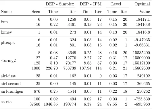
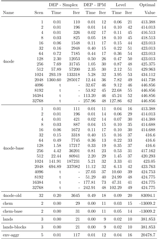
Table 4: Performance of DEP solution methods and level-regularised decomposition

t - time limit, m - insufficient memory, n - numerical difficulties

DEP - Simplex DEP - IPM Level Optimal

Name Scen Time Iter Time Iter Time Iter Value

fxm 6 0.06 1259 0.05 17 0.15 20 18417.1

16 0.22 3461 0.13 23 0.15 20 18416.8

fxmev 1 0.01 273 0.01 14 0.13 20 18416.8

pltexpa 6 0.01 324 0.03 14 0.02 1 -9.47935

16 0.01 801 0.08 16 0.02 1 -9.66331

stormg2

8 0.08 3649 0.25 28 0.16 20 15535200 27 0.47 12770 2.27 27 0.31 17 15509000 125 5.10 70177 8.85 57 0.93 17 15512100 1000 226.70 753739 137.94 114 6.21 21 15802600

airl-first 25 0.01 162 0.01 9 0.03 17 249102

airl-second 25 0.00 145 0.01 11 0.03 17 269665

airl-randgen 676 0.25 4544 0.05 11 0.22 18 250262

assets 100 0.02 494 0.02 17 0.03 1 -723.839

37500 1046.85 190774 6.37 24 87.55 2 -695.963

(21)

Table 4: Performance of DEP solution methods and level-regularised decomposition (continued)

4node

1 0.01 110 0.01 12 0.06 21 413.388

2 0.01 196 0.01 14 0.10 42 414.013

4 0.01 326 0.02 17 0.11 45 416.513

8 0.03 825 0.05 18 0.10 45 418.513

16 0.06 1548 0.11 17 0.15 44 423.013 32 0.16 2948 0.40 15 0.22 51 423.013 64 0.72 7185 0.44 17 0.36 54 423.013 128 2.30 12053 0.50 26 0.47 50 423.013 256 7.69 31745 1.05 30 0.87 48 425.375 512 57.89 57200 2.35 30 2.12 51 429.963 1024 293.19 133318 5.28 32 3.95 53 434.112 2048 1360.60 285017 12.44 36 7.82 49 441.738

4096 t - 32.67 46 9.12 46 446.856

8192 t - 53.82 45 22.68 55 446.856

16384 t - 113.20 46 45.24 52 446.856

32768 t - 257.96 48 127.86 62 446.856

4node-base

1 0.01 111 0.01 11 0.04 16 413.388

2 0.01 196 0.01 14 0.06 29 414.013

4 0.01 421 0.02 14 0.07 30 414.388

8 0.03 887 0.04 15 0.10 35 414.688

16 0.06 1672 0.11 17 0.10 30 414.688

32 0.15 3318 0.40 15 0.16 37 416.6

64 0.49 7745 0.36 13 0.22 33 416.6

128 1.58 17217 0.33 19 0.35 37 416.6 256 4.42 36201 0.81 23 0.53 31 417.162 512 22.44 80941 2.20 29 1.45 37 420.293 1024 141.91 187231 5.21 32 3.33 41 423.05 2048 694.89 337082 11.12 32 6.13 42 423.763

4096 t - 27.03 37 10.60 39 424.753

8192 t - 51.29 40 24.99 48 424.775

16384 t - 177.81 73 47.31 41 424.775

32768 t - 242.91 48 102.29 49 424.775

4node-old 32 0.20 3645 0.49 18 0.09 20 83094.1

chem 2 0.00 29 0.00 11 0.03 15 -13009.2

chem-base 2 0.00 31 0.00 11 0.05 14 -13009.2

lands 3 0.00 21 0.00 9 0.02 10 381.853

lands-blocks 3 0.00 21 0.00 9 0.02 10 381.853

env-aggr 5 0.01 117 0.01 12 0.04 16 20478.7

(22)

Table 4: Performance of DEP solution methods and level-regularised decomposition (continued)

env-first 5 0.01 112 0.01 11 0.02 1 19777.4

env-loose 5 0.01 112 0.01 12 0.02 1 19777.4

env

15 0.01 321 0.01 16 0.05 15 22265.3

1200 1.38 23557 1.44 34 1.73 15 22428.9 1875 2.90 36567 2.60 34 2.80 15 22447.1 3780 11.21 73421 7.38 40 5.47 15 22441 5292 20.28 102757 12.19 42 7.67 15 22438.4 8232 62.25 318430 m - 12.58 15 22439.1 32928 934.38 1294480 m - 75.67 15 22439.1 env-diss-aggr 5 0.01 131 0.01 9 0.05 22 15963.9 env-diss-first 5 0.01 122 0.01 9 0.04 12 14794.6 env-diss-loose 5 0.01 122 0.01 9 0.03 5 14794.6

env-diss

15 0.01 357 0.02 13 0.10 35 20773.9

1200 1.96 26158 1.99 50 2.80 35 20808.6 1875 4.41 40776 3.63 53 4.49 36 20809.3 3780 16.94 82363 9.32 57 8.87 36 20794.7 5292 22.37 113894 16.17 66 12.95 38 20788.6 8232 70.90 318192 m - 22.49 41 20799.4 32928 1369.97 1296010 m - 112.46 41 20799.4