Research Collection
Working Paper
Solving Zero-Sum Games through Alternating Projections
Author(s):
Anagnostides, Ioannis; Penna, Paolo Publication Date:
2020-09
Permanent Link:
https://doi.org/10.3929/ethz-b-000456982
Rights / License:
In Copyright - Non-Commercial Use Permitted
This page was generated automatically upon download from the ETH Zurich Research Collection. For more information please consult the Terms of use.
Solving Zero-Sum Games through Alternating Projections
Ioannis Anagnostides ianagnost@student.ethz.ch
Paolo Penna
paolo.penna@inf.ethz.ch
Abstract
In this work, we establish near-linear and strong convergence for a natural first-order iterative algorithm that simulates Von Neumann’s Alternating Projections method in zero- sum games. First, we provide a precise analysis of Optimistic Gradient Descent/Ascent (OGDA) – an optimistic variant of Gradient Descent/Ascent [DISZ17] – forunconstrained bilinear games, extending and strengthening prior results along several directions. Our characterization is based on a closed-form solution we derive for the dynamics, while our results also reveal several surprising properties. Indeed, our main algorithmic contribution is founded on a geometric feature of OGDA we discovered; namely, the limit points of the dynamics are the orthogonal projection of the initial state to the space of attractors.
Motivated by this property, we show that the equilibria for a natural class ofconstrained bilinear games are the intersection of the unconstrained stationary points with the cor- responding probability simplexes. Thus, we employ OGDA to implement an Alternating Projections procedure, converging to an -approximate Nash equilibrium in O(loge 2(1/)) iterations. Although our algorithm closely resembles the no-regret projected OGDA dy- namics, it surpasses the optimal no-regret convergence rate of Θ(1/) [DDK15], while it also supplements the recent work in pursuing last-iterate guarantees in saddle-point problems [DP18a,MLZ+19]. Finally, we illustrate an – in principle – trivial reduction from any game to the assumed class of instances, without altering the space of equilibria.
arXiv:2010.00109v1 [math.OC] 30 Sep 2020
1 Introduction
The classical problem of finding a Nash equilibrium in multi-agent systems has been a topic of prolific research in several areas, including Mathematics, Economics, Algorithmic Game Theory, Optimization [Nas50,Sio58,DGP06,NRTV07,Nes05] and more recently Machine Learning in the context of Generative Adversarial Networks [GPAM+14,ACB17] and multi-agent reinforce- ment learning [HW98]. The inception of this endeavor can be traced back to Von Neumann’s celebrated min-max theorem, which asserts that
x∈∆minn
y∈∆maxm
xTAy= max
y∈∆m
x∈∆minn
xTAy, (1)
where ∆n and ∆m are probability simplexes and A the matrix of the game. To be more pre- cise, (1) implies that an equilibrium – a pair of randomized strategies such that neither player can benefit from a unilateral deviation – always exists; yet, the min-max theorem does not inform us on whether natural learning algorithms can converge to this equilibrium with a rea- sonable amount of computational resources. This question has given rise to intense research, commencing from the analysis of fictitious play by J. Robinson [Rob51] and leading to the development of the no-regret framework [CBL06, BM05,AHK12]. However, an unsatisfactory characteristic of these results is that the minimax pair is only obtained in an average sense, without any last-iterate guarantees. Indeed, a regret-based analysis cannot distinguish between a self-stabilizing system and one with recurrent cycles. In this context, it has been exten- sively documented that limit cycles – or more preciselyPoincar´e recurrences – are persistent in broad families of no-regret schemes, such as Mirror Descent and Follow-The-Regularized-Leader [MPP18,PPP17,PP16,PS14].
Figure 1: The behavior of Projected Gradient Descent (leftmost image) and Entropic - or Exponentiated - Descent (rightmost image) for the game of matching pennies. Symbol ’x’ represents the unique (uniform) equilibrium, while the red point corresponds to the initial state of the system. Although both algorithms suffer no-regret – as instances of Mirror Descent, they exhibit cyclic behavior around the equilibrium.
The crucial issue of last-iterate convergence was addressed by Daskalakis et al. [DISZ17]
in two-player and zero-sum games in the context of training Generative Adversarial Networks.
In particular, they introduced Optimistic Gradient Descent/Ascent (henceforth abbreviated as OGDA), a simple variant of Gradient Descent/Ascent (GDA) that incorporates a prediction term on the next iteration’s gradient, and they proved point-wise convergence in unconstrained bilinear min-max optimization problems. It is clear that the stabilizing effect of optimism is of fundamental importance within the scope of Game Theory, which endeavors to study and indeed, control dynamical systems of autonomous agents. However, despite recent follow-up works [LS19,MOP20], an exact characterization of OGDA and its properties remains largely
unresolved. In this context, the first part of our work provides a precise analysis of OGDA, resolving several open issues and illuminating surprising attributes of the dynamics.
Naturally, the stability of the learning algorithm has also emerged as a critical consideration in the more challenging and indeed, relevant case of constrained zero-sum – or simply zero- sum – games. Specifically, Daskalakis and Panageas [DP18a] analyzed an optimistic variant of Multiplicative Weight Updates and they showed last-iterate convergence in games with a unique equilibrium; yet, the rate of convergence was left entirely open. The same issue arises in the analysis of Optimistic Mirror Descent by Mertikopoulos et al. [MLZ+19]; in the parlance of the Variational Inequality framework, the main challenge is that the operator – the flow – in bilinear games is weakly-monotone – just as linear functions are convex in a weak sense – and standard tools appear to be of no use. The main algorithmic contribution of our paper is a natural variant of projected OGDA that simulates an Alternating Projections procedure;
as such, it exhibits a surprising near-linear and strong convergence in constrained games. Our approach is based on a non-trivial geometric property of OGDA: the limit points are – under certain hypotheses – positively correlated with the Nash equilibria of the constrained game.
Although our algorithm is not admitted in the no-regret framework, it is based entirely on the no-regret (projected) OGDA dynamics. Importantly, our techniques and the connections we establish could prove useful in the characterization of the convergence’s rate in other algorithms.
Related Work Our work follows the line of research initiated by [DISZ17]; one of their key results was proving through an inductive argument that OGDA, a simple variant of GDA, exhibits point-wise convergence to the space of Nash equilibria for any unconstrained bilinear game. The convergence rate was later shown to be linear in [LS19]. Moreover, this result was also proven in [MOP20], where the authors illustrated that OGDA can be examined as an approximate version of the proximal point method; through this prism, they also provided a convergence guarantee for convex-concave games. However, both of the aforementioned works consider only the special case of a square matrix with full-rank.
The underlying technique of optimism employed in OGDA has gradually emerged in the fields of Online Learning and Convex Optimization [SALS15, SL14, WA18], and has led to very natural algorithmic paradigms. More precisely, optimism consists of exploiting the pre- dictability or smoothness of the future cost functions, incorporating additional knowledge in the optimization step. In fact, in the context of zero-sum games, this technique has guided the optimal no-regret algorithms, leading to a regret of Θ(1/T), whereT the number of iterations [DDK15,RS13].
It is well-established that a minimax pair in zero-sum games can be computed in a central- ized manner via an induced Linear Program (LP). In particular, interior point methods and variants of Newton’s method are known to exhibit very fast convergence, even super-linear – e.g. O(log log (1/)); see [PW00, Wri97]. We also refer to [Reb09] for the ellipsoid method, another celebrated approach for solving LPs. However, these algorithms are not commonly used in practice for a number of reasons. Indeed, first-order methods have dominated the at- tention both in the literature and in practical applications, mainly due to their simplicity, their robustness - e.g. noise tolerance - and the limited computational cost of implementing a single step, relatively to the aforementioned algorithms [Rud16]. Another reference point for our work should be Nesterov’s iterative algorithm [Nes05] that strongly converges to an -approximate equilibrium after O(1/) iterations.
In a closely related work, Mertikopoulos et. al [MLZ+19] established convergence for pro- jected OGDA and Extra-Gradient dynamics. Our main algorithm is also established as pro- jected variant of OGDA, but instead of projecting after a single step, the projection is per- formed after multiple iterations. A no-regret analysis of Optimistic Mirror Descent can be found in [KHSC18]. For a characterization of the stationary points of GDA and OGDA and their nexus to Nash equilibria beyond convex-concave settings we refer to [DP18b]. Finally,
several algorithms have been proposed specifically for solving saddle-point problems; we refer to [ADLH19,SA19,MJS19] and references thereof.
Our Contributions In the first part of our work (Section3), we provide a thorough and com- prehensive analysis of Optimistic Gradient Descent/Ascent in unconstrained bilinear games.
Specifically, we first derive an exact and concise solution to the dynamics in Subsection 3.1;
through this result, we establish convergence from any initial state (Theorem 3.1). Note that the guarantee in [DISZ17] was only shown for cherry-picked initial conditions, an unnatural restriction for a linear dynamical system. We also show that the rate of convergence is linear (Corollary 5.1); this was proved in follow-up works [LS19, MOP20] for the specific case of a square non-singular matrix. Our analysis is also tighter with respect to the learning rate, yield- ing a broader stability region compared to the aforementioned works. In fact, in Proposition3.2 we derive the exact rate of convergence with respect to the learning rate and the spectrum of the matrix. One important implication is that within our stable region, increasing the learning rate will accelerate the convergence of the system, a property which is of clear significance in practical implementations of the algorithm. Proposition 3.2 also implies a surprising disconti- nuity on the behavior of the system: an arbitrarily small noise may dramatically alter the rate of convergence (see Appendix B). Another counter-intuitive consequence of our results is that OGDA could actually converge with negative learning rate. Finally, we reformulate our solu- tion to illustrate the inherent oscillatory components in the dynamics, albeit with a vanishing amplitude (AppendixD). Throughout Section3, we mainly use techniques and tools from Lin- ear Algebra and Spectral Analysis – such as the Spectral Decomposition, while we also derive several non-trivial identities that could of independent interest. We consider our analysis to be simpler than the existing ones.
In the second part, we turn to constrained games and we commence (in Section4) by showing that the Nash equilibria are the intersection of the unconstrained stationary points with the corresponding probability simplexes, assuming that the value of the (constrained) game is zero and that there exists an interior equilibrium (see Proposition4.3). Thus, under these conditions, the optimal strategies can be expressed as the intersection of two closed and convex sets and hence, they can be determined through Von Neumann’s Alternating Projections method. In this context, our algorithm (Algorithm 1) is based on a non-trivial structural property of OGDA:
the limit points are the orthogonal projection of the initial state to the space of attractors (see Theorem3.2for a formal statement). As a result, OGDA is employed in order to implement the Alternating Projections procedure. We show with simple arguments that our algorithm yields an -approximate Nash equilibrium with O(loge 2(1/)) iterations (Theorem 5.2). To the best of our knowledge, the rate of convergence of our algorithm outperforms the known first-order methods; surprisingly, although our algorithm closely resembles the no-regret projected OGDA dynamics, it surpasses the optimal no-regret convergence rate of Θ(1/) [DDK15].
Moreover, our algorithm also converges in the last-iterate sense, supplementing the recent works in this particular direction [MLZ+19,DP18a]; however, unlike the aforementioned results, our analysis gives a precise and parametric characterization of the convergence’s rate; thus, our techniques could prove useful in the analysis of other dynamics. We also believe that the variant of projected Gradient Descent we introduced, namely performing the projection to the feasible set only after multiple iterations, could be of independent interest in the regime of Optimization.
The main caveat of our approach is that we consider (constrained) games that have an interior equilibrium and value v = 0; we ameliorate this limitation by showing an – in principle – trivial reduction from any arbitrary game to the assumed class of instances. We emphasize on the fact that the equilibria of the game remain – essentially – invariant under our reduction.
Importantly, our approach offers a novel algorithmic viewpoint on a fundamental problem in Optimization and Game Theory.
Alternating Projections Our main algorithm (Algorithm 1) is an approximate instance of Von Neumann’s celebrated method of Alternating Projections. More precisely, if H1 and H2 are closed subspaces of a Hilbert space H, he showed that alternatively projecting to H1 and H2 will eventually converge in norm to the projection of the initial point to H1 ∩ H2. This method has been applied in many areas, including Stochastic Processes [AA68], solving linear equations [Tan71] and Convex Optimization [BB96, Bre67, BV04], while it was also independently discovered by Wiener [Wie55]. Moreover, a generalization of this algorithm to multiple closed subspaces was given by Halperin [Hal62], introducing the method of cyclic alternating projections. The rate of convergence was addressed in [Aro50,BGM10,KW88], and in particular it was shown that for 2 closed subspaces – and under mild assumptions – the rate of convergence is linear and parameterized by theFriedrichs anglebetween the subspaces. Beyond affine spaces, Von Neumann’s method also converges when the sets are closed and convex 1, assuming a non-empty intersection. In fact, certain results in this domain are applicable even when the intersection between the subsets is empty; e.g. see Dijkstra’s projection algorithm.
2 Preliminaries
Nash equilibrium Consider a continuously differentiable function f : X × Y 7→ R that represents the objective function of the game, with f(x,y) the payoff of player X to player Y under strategiesx∈ X andy∈ Y respectively. A pair of strategies (x∗,y∗)∈ X × Y is a Nash equilibrium – or asaddle-point of f(x,y) – if ∀(x,y)∈ X × Y,
f(x∗,y)≤f(x∗,y∗)≤f(x,y∗). (2) A pair of strategies (x∗,y∗) will be referred to as an -approximate Nash equilibrium if it satisfies (2) with up to an additive error. We may sometimes refer to player X as the minimizer and playerY as the maximizer. Throughout this paper, we consider exclusively the case off(x,y) =xTAy, while in a constrained game – or simply (finite) zero-sum game in the literature of Game Theory – we additionally require that X = ∆n and Y = ∆m.
Optimistic Gradient Descent/Ascent Let us focus on the unconstrained case, i.e. X =Rn and Y = Rm. The most natural optimization algorithm for solving the induced saddle-point problem is by performing simultaneously Gradient Descent on x and Gradient Ascent on y;
formally, if η > 0 denotes some positive constant – typically referred to as the learning rate, GDA can be described as follows:
xt=xt−1−η∇xf(xt−1,yt−1),
yt=yt−1+η∇yf(xt−1,yt−1). (3) However, there are very simple examples where the system of equations (3) diverges; for instance, when f(x, y) = xy with x, y ∈ R and (x0, y0) 6= (0,0), GDA is known to diverge for any learning rate η > 0. This inadequacy has motivated optimistic variants of GDA that incorporate some prediction on the next iteration’s gradient through the regularization term (recall that Gradient Descent can be viewed as an instance of Follow-The-Regularized-Leader (FTRL) with Euclidean regularizer [Sha12]). With OGDA we refer to the optimization variant that arises when the prediction of the next iteration’s gradient is simply the previously observed gradient; this yields the following update rules:
xt=xt−1−2η∇xf(xt−1,yt−1) +η∇xf(xt−2,yt−2),
yt=yt−1+ 2η∇yf(xt−1,yt−1)−η∇yf(xt−2,yt−2). (4)
1In this context, the method of alternating projections is sometimes referred to as projection onto convex sets or POCS
A probability vector p is referred to as interior ifpi >0,∀i; subsequently, an equilibrium point (x,y) ∈ ∆n ×∆m is called interior if both x and y are interior probability vectors.
Let amax the entry of A with maximum absolute value; it follows that the bilinear objective function f(x,y) = xTAy is |amax|-Lipschitz continuous in ∆n×∆m. Note that rescaling the entries of the matrix by a positive constant does not alter the game; for Theorem5.2 we make the normative assumption that every entry is multiplied by 1/|amax|, so that the objective function is 1-Lipschitz. A set isclosed if and only if it contains all of its limit points. Moreover, a subset of a Euclidean space is compact if and only if it is closed and bounded (Heine-Borel theorem).
Hilbert Spaces Although this paper deals with optimization in finite-dimensional Euclidean spaces, we wish to present the Alternating Projections method in its general form in arbitrary Hilbert spaces (see Theorem 5.1). In this context, we review some basic concepts that the reader may need. A Hilbert spaceHis an inner product and complete – every Cauchy sequence converges – metric space. The norm is defined as||u||=p
hu, ui, where h·,·idenotes the inner product inH. Moreover, the distance betweenu, v∈ His defined in terms of norm byd(u, v) =
||u−v||, while d(u, S) = infv∈Sd(u, v) – for some non-empty set S ⊆ H. Also recall from Hilbert’s projection theorem that if C is a non-empty, closed and convex set in a Hilbert space H, the projection of any pointu∈ H toC is uniquely defined as PC(u) = arg minv∈C||u−v||.
Definition 2.1. A sequence{un}∞0 on a Hilbert spaceHis said to converge linearly2 tou∗∈ H with rate λ∈(0,1) if
n→∞lim
||un+1−u∗||
||un−u∗|| =λ. (5)
Notation We denote with A ∈ Rn×m the matrix of the game and with x ∈ X,y ∈ Y the players’ strategies. With ∆k we denote the k-dimensional probability simplex. We use t and k as discrete time indexes, while the variables i, j, k, t will be implied to be integers, without explicitly stated as such. We use Ik and 0k×` to refer to the identity matrix of sizek×k and the zero matrix of size k×` respectively; when k=`we simply write 0k instead of 0k×k. We also use 1k×` to denote the k×` matrix with 1 in every entry, while we sometimes omit the dimensions when they are clear from the context. The vector norm will refer to the Euclidean norm || · ||2, while we denote with ||S|| the spectral norm of S, that is, the square root of the maximum eigenvalue ofSTS. Finally, N(S) represents the null space of matrix S.
3 Characterizing OGDA
Throughout this section, we analyze Optimistic Gradient Descent/Ascent for unconstrained and bilinear games, i.e. f(x,y) =xTAy,X =Rn andY =Rm.
3.1 Solving the Dynamics
In this subsection, we derive a closed-form and concise solution to the OGDA dynamics. First, consider some arbitrary initial conditions for the players’ strategiesx−1,x0 ∈Rn andy−1,y0 ∈ Rm. When the objective function is bilinear, the update rules of OGDA (4) can be formulated fort≥1 as
xt=xt−1−2ηAyt−1+ηAyt−2,
yt=yt−1+ 2ηATxt−1−ηATxt−2. (6)
2To avoid confusion, we should mention that linear convergence in iterative methods is usually referred to as exponential convergence in discretization methods.
These equations can be expressed more concisely in matrix form:
xt yt
=
In −2ηA 2ηAT Im
xt−1
yt−1
+
0n ηA
−ηAT 0m
xt−2
yt−2
. (7)
In correspondence to the last expression, let us introduce the following matrices:
zt= xt
yt
, B=
In −2ηA 2ηAT Im
, C =
0n ηA
−ηAT 0m
. (8)
With this notation, Equation (7) can be re-written as
zt=Bzt−1+Czt−2. (9)
Equation (9) induces a second-order and linear recursion in matrix form; hence, its solution can be derived through a standard technique. In particular, it is easy to verify that (9) can be equivalently reformulated as
zt zt−1
=
B C In+m 0n+m
zt−1
zt−2
= ∆t z0
z−1
, (10)
where
∆ =
B C In+m 0n+m
. (11)
As a result, we have reduced solving the OGDA dynamics to determining matrix ∆t. To this end, first note that the block sub-matrices of ∆ have the same dimensions (n+m)×(n+m). In addition, every couple of these sub-matrices satisfies the commutative property; indeed, we can verify thatBC =CB and hence, every possible multiplicative combination will also commute.
Thus, we can invoke for the sub-matrices polynomial identities that apply for scalar numbers.
In this direction, we establish the following claim:
Lemma 3.1. Consider a matrix R∈R2×2 defined as R=
b c 1 0
. (12)
Then, for any k≥2,
Rk=
bk2c
X
i=0
k−i i
bk−2ici
bk−12 c
X
i=0
k−i−1 i
bk−2i−1ci+1
bk−12 c
X
i=0
k−i−1 i
bk−2i−1ci
bk−22 c
X
i=0
k−i−2 i
bk−2i−2ci+1
. (13)
We refer to Appendix E.1 for a proof of this lemma; essentially it follows from the Cay- ley–Hamilton theorem and simple combinatorial arguments. In addition, we can also express the power of matrixR– as defined in Equation (12) – using the spectral decomposition – or the more general Singular Value Decomposition (SVD) method, which yields the following identity:
Proposition 3.1. For any b, c∈Rsuch that b2+ 4c >0 and k≥0,
bk2c
X
i=0
k−i i
bk−2ici = 1
√b2+ 4c
b+√ b2+ 4c 2
!k+1
− b−√ b2+ 4c 2
!k+1
. (14)
This identity can be seen as a non-trivial variant of the celebrated binomial theorem. For a proof and connections to the Fibonacci series we refer to Appendix E.2. Next, we employ the previous results to derive analogous expressions for the matrix case.
Corollary 3.1. For any k≥2,
∆k=
bk2c
X
i=0
k−i i
Bk−2iCi
bk−12 c
X
i=0
k−i−1 i
Bk−2i−1Ci+1
bk−12 c
X
i=0
k−i−1 i
Bk−2i−1Ci
bk−22 c
X
i=0
k−i−2 i
Bk−2i−2Ci+1
. (15)
This claim follows directly from Lemma 3.1 and the fact that the square matrices B and C commute. As a result, we can apply this corollary to Equation (10) in order to derive the following expression for the dynamics of OGDA:
xt
yt
=
bt2c
X
i=0
t−i i
Bt−2iCi
x0
y0
+
bt−12 c
X
i=0
t−i−1 i
Bt−2i−1Ci+1
x−1
y−1
. (16) Let us assume that
Qt=
bt
2c
X
i=0
t−i i
Bt−2iCi. (17)
Then, Equation (16) can be written as xt
yt
=Qt x0
y0
+Qt−1C x−1
y−1
. (18)
Therefore, the final step is to provide a more compact expression for Qt. Note that the convergence of the dynamics reduces to the convergence ofQt. To this end, we will establish a generalized version of Proposition 3.1that holds for matrices. First, let
T =B2+ 4C =
In−4η2AAT 0n×m
0m×n Im−4η2ATA
. (19)
Let us assume that γ = ||A|| = ||AT||; recall that ||AAT|| = ||ATA|| = γ2. Naturally, we consider the non-trivial case whereγ 6= 0.
Lemma 3.2. For any learning rate η <1/(2γ), matrixT is positive definite.
We provide a proof for this claim in Appendix E.3. As a result, for any sufficiently small learning rate, the (positive definite) square root of matrixT – the principal square rootT1/2 – is well defined, as well as its inverse matrixT−1/2.
Lemma 3.3. Consider a learning rate η <1/(2γ); then, matrices B and T1/2 commute.
Corollary 3.2. For any η <1/(2γ), Qt=T−1/2
B+T1/2 2
!t+1
− B−T1/2 2
!t+1
. (20)
This corollary follows directly from the previous lemmas and Proposition 3.1. Therefore, if we replace the derived expression ofQt in Equation (18) we obtain a closed-form and succinct solution for the OGDA dynamics. In the following sections we employ this result to characterize the behavior of the dynamics.
3.2 Convergence of the Dynamics
It is clear that analyzing the convergence of OGDA reduces to investigating the asymptotic behavior of Qt; in particular, we can prove the following theorem:
Theorem 3.1. For any learning rate η <1/(2γ), OGDA converges from any initial state.
Sketch of Proof. We give a high-level sketch of our techniques. For a rigorous proof we refer to Appendix E.5. First, a sufficient condition for the claim to hold is that the powers of both matrices (B+T1/2)/2 and (B−T1/2)/2 converge, which is tantamount to showing that their spectrum resides within the unit circle. In this context, although the spectrum of B and T1/2 can be determined as a simple exercise, the main complication is that the spectrum of the sum of matrices cannot be – in general – characterized from the individual components. Nonetheless, we show that B and T1/2 are simultaneously diagonalizable and that their eigenvalues are in a particular correspondence.
Remark Throughout our analysis we made the natural assumption that the learning rate η is positive. However, our proof of convergence in Theorem 3.1 (see Appendix E.5) remains valid when |η|<1/(2γ), implying a very counter-intuitive property: OGDA can actually con- verge with negative learning rate! Of course, this is very surprising since performing Gradient Descent/Ascent with negative learning rate leads both players to the direction of the (locally) worst strategy. Perhaps, the optimistic term negates this intuition.
Corollary 3.3. For any learning rate η <1/(2γ), OGDA exhibits linear convergence.
We can also provide an exact characterization of the convergence’s rate of OGDA with respect to the learning rate and the spectrum of the matrix of the game A, as stated in the following proposition.
Proposition 3.2. Let λmin be the minimum non-zero eigenvalue of matrix 4η2AAT; then, assuming that η <1/(2γ), the convergence rate of OGDA is e(λmin), where
e(λ) = s
1 +√ 1−λ
2 . (21)
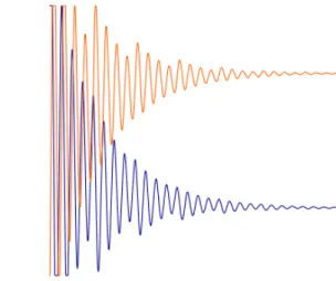
For the proof of the claim we refer to Appendix E.6. An important consequence of this proposition is that whileη <1/(2γ), increasing the learning rate will accelerate the convergence of the dynamics. Moreover, Proposition3.2implies a rather surprising discontinuity on the rate of convergence (see Appendix B). We also refer to AppendixDfor a precise characterization of the inherent oscillatory component in the dynamics. This subsection is concluded with a simple example, namelyf(x, y) =xywithx, y∈R. Figure2illustrates the impact of the learning rate to the behavior of the system.
3.3 Limit Points of the Dynamics
Having established the convergence of the dynamics, the next natural question that arises relates to the characterization of the limit points. We initiate our analysis with the following proposition.
Proposition 3.3. A pair of strategies (x∗,y∗) ∈ Rn×Rm constitutes a Nash equilibrium for the unconstrained bilinear game if and only if Ay∗ =0 and ATx∗ =0, that is y∗ ∈ N(A) and x∗ ∈ N(AT).
As a result, it is easy to show that when the players’ strategies converge, the limit points will constitute a Nash equilibrium, as stated in the following proposition.
Figure 2: The trajectories of the players’ strategies throughout the evolution of the game; the blue color corresponds to a positive learning rate, while the orange to a negative one. We know from Theorem3.1 that when η < 1/2 the dynamics converge; moreover, it follows from Proposition 3.2 that while the learning rate gradually increases, without exceeding the threshold ofη= 1/2, the system exhibits faster convergence and limited oscillatory behavior. Remarkably, a negative learning rate simply leads to a reflection of the trajectories.
Proposition 3.4. If OGDA converges, the limit points are Nash equilibria.
This claim follows very easily from the structure of OGDA and Proposition 3.3; we refer to AppendixE.8for the proof. Proposition 3.4 asserts that the limit pointsx∞ and y∞ reside in the left and right null space ofArespectively – assuming convergence. In fact, we can establish a much more precise characterization. In particular, let r the rank of matrix A; from the fundamental theorem of Linear Algebra it follows that dimN(A) = m−r and dimN(AT) = n−r. We shall prove the following theorem.
Theorem 3.2. Let {y1,y2, . . . ,ym−r} an orthonormal basis for N(A) and {x1,x2, . . . ,xn−r} an orthonormal basis forN(AT); then, assuming thatη <1/(2γ),y∞ is the orthogonal projec- tion of y0 to N(A) and x∞ is the orthogonal projection of x0 to N(AT), that is
t→∞lim yt=
m−r
X
i=1
hy0,yiiyi, (22)
t→∞lim xt=
n−r
X
i=1
hx0,xiixi. (23) The proof follows from our solution to the OGDA dynamics and simple calculations (see AppendixE.9). This theorem provides a very important and natural insight on the limit points of OGDA: the dynamics converge to the attractor which is closer to the initial configuration (x0,y0). An important implication of this property is that we can use OGDA in order to implement the projection to the null space ofA – for theyplayer – and the null space ofAT – for thex player.
4 Characterization of Nash equilibria in Constrained Games
The main purpose of this section is to correlate the equilibria between constrained and un- constrained games. Specifically, if v represents the value of a constrained game that possesses
an interior equilibrium, we show that (x,y) ∈ ∆n×∆m is a Nash equilibrium if and only if Ay =v1 and ATx=v1; thus, whenv = 0 the stationary points will derive from the intersec- tion of the null space ofAand AT with the corresponding probability simplexes, establishing a clear connection with the saddle-points of the corresponding unconstrained bilinear game (recall Proposition3.3). First, let us introduce the following notation:
NE ={(x∗,y∗)∈∆n×∆m : (x∗,y∗) is an equilibrium of the constrained game}. (24) Consider two pairs of Nash equilibria; a very natural question is whether a mixture – a convex combination – of these pairs will also constitute a Nash equilibrium. This question is answered in the affirmative in the following propositions.
Proposition 4.1. There exist ∆∗n ⊆ ∆n and ∆∗m ⊆ ∆m, with ∆∗n,∆∗m 6= ∅, such that NE =
∆∗n×∆∗m.
Sketch of Proof. The claim follows from a simple decoupling argument; in particular, it is easy to see that
(x∗,y∗)∈NE ⇐⇒
x∗ ∈arg min
x∈∆n y∈∆maxm
xTAy y∗ ∈arg max
y∈∆m x∈∆minn
xTAy
⇐⇒
( x∗ ∈∆∗n y∗∈∆∗m
)
, (25)
where ∆∗n and ∆∗mconstitute the set of optimal strategies, as defined in (25). Finally, note that Von Neumann’s min-max theorem implies that ∆∗n and ∆∗m are non-empty.
Proposition 4.2. The sets of optimal strategies ∆∗n and∆∗m are convex.
Proof. Let x∗1,x∗2 ∈∆∗n and some λ∈[0,1]. It suffices to show thatλx∗1+ (1−λ)x∗2∈∆∗n; the convexity of ∆∗m will then follow from an analogous argument. Indeed, we have that
y∈∆maxm(λx∗1+ (1−λ)x∗2)TAy≤λ max
y∈∆m(x∗1)TAy+ (1−λ) max
y∈∆m(x∗2)TAy
≤ max
y∈∆m
xTAy, ∀x∈∆n, where the last line follows from x∗1,x∗2 ∈∆∗n; thus, λx∗1+ (1−λ)x∗2∈∆∗n.
While the previous statements hold for any arbitrary game, the following proposition will require two separate hypotheses; after we establish the proof we will illustrate that these as- sumptions are – in principle – generic, in the sense that every game can be reduced with simple operations to the assumed form, without – essentially – altering the space of equilibria.
Proposition 4.3. Consider a constrained zero-sum game with an interior equilibrium and value v= 0; then, it follows that
NE = ∆n∩ N(AT)
×(∆m∩ N(A)). (26) Reduction Finally, we shall address the assumptions made in the last proposition. First, consider a matrixA0 that derives fromAwith the addition of a constantcin every entry; then, forx∈∆n andy∈∆m, it follows that
xTA0y=xT(A+c1n×m)y=xTAy+c. (27)
Therefore, the addition of c in every entry of the matrix does not alter the space of Nash equilibria; it does, however, change the value of the game by an additive constantc. As a result, if we add in every entry of a matrix the value −v, the game that arises has a value of zero.
As a corollary of Proposition 4.3, (x,y) is a Nash equilibrium pair – in a game where there exists an interior equilibrium – if and only if Ay =v1 and ATx =v1. Furthermore, consider a game that does not possess an interior equilibrium. In particular, let us assume that every x∗ ∈∆∗nresides in the boundary of ∆n. Then, it follows that there exists some action for player xwith zero probability for everyx∗ ∈∆∗n. Indeed, if we posit otherwise Proposition4.2implies the existence of an interior probability vector x∗ ∈ ∆∗n, contradicting our initial hypothesis.
Thus, we can iteratively remove every row from the matrix that corresponds to such actions, until no such row exists. It is easy to see that this operation does not have an impact on the Nash equilibria of the game, modulo some dimensions in which the player always assigns zero probability mass. Finally, we can apply – if needed – a similar process for the column player and obtain a game with an interior equilibrium. In other words, games without interior equilibria are reducible, in the sense that the ’unsound’ actions from either the row or the column player can be removed without altering the game under optimal play.
Remark It is important to point out that this reduction argument is merely a thought exper- iment, illustrating that the games we consider capture – at least in some sense – the complexity of the entire class; yet, it does not provide an appropriate reduction since unknown components – such as the value of the game – are used. We leave as an open question whether it is possible to incorporate this reduction in our iterative algorithm.
5 Alternating Projections
Based on the properties we have established in the previous sections, we provide an algorithm that (strongly) converges to the space of Nash equilibria in constrained games. Throughout this section, we will require that the value of the game is zero and that there exists an interior equilibrium (see AppendixCon why these assumptions are necessary); under these hypotheses, we have a strong characterization of the optimal strategies (Proposition4.3): ∆∗n= ∆n∩N(AT) and ∆∗m = ∆m∩ N(A). As a result, we can employ an Alternating Projections scheme.
Complexity of Projection It is important to point out that the complexity of implementing a projection to a non-empty, convex and closed set C depends primarily on the structure of C. Indeed, identifying the projection to an arbitrary set constitutes a non-trivial optimization problem of its own. For this reason, we need OGDA to implement the projection to the null space of Aand AT. On the other hand, we make the standard assumption that the projection to the probability simplex is computed in a single iteration.
In this context, our main algorithm constitutes a projected variant of OGDA; specifically, instead of projecting after a single step, we simulate multiplesteps Ts of the OGDA algorithm, before finally performing the projection. This process will be repeated for Tp cycles. We will assume for simplicity that OGDA is initialized with x−1 =0 and y−1 =0, without having an impact on its limit points (Theorem3.2). Recall from Theorem3.2that OGDA converges to the projection of the initial conditions x0 and y0 to the left and right null space of A respectively.
Thus, our algorithm essentially performs – for sufficiently large Ts – alternate projections in N(AT) and ∆n in the domain of the x player, and in N(A) and ∆m in the domain of the y player. In this sense, it can be viewed as an approximate instance of Alternating Projections.
We state the following theorem in order to illustrate the robustness of this method to arbitrary Hilbert spaces.
Algorithm 1:Alternating Projections Result: Approximate Nash equilibrium
Input: matrix of the gameA, (xp0,y0p)∈∆n×∆m, learning rateη for k:= 1,2, . . . , Tp do
x0 :=xpk−1; y0 :=ypk−1;
fort:= 1,2, . . . , Ts do
xt:=xt−1−2ηAyt−1+ηAyt−2; yt:=yt−1+ 2ηATxt−1−ηATxt−2; end
xpk :=P∆n(xTs);
ykp :=P∆m(yT
s);
end
return (xpTp,yTpp);
Theorem 5.1. Let M and N denote closed and convex subsets of a Hilbert space H with non- empty intersection and I ∈ H. If one of the sets is compact 3, the method of Alternating Projections converges in norm to a point in the intersection of the sets; that is, ∃L∈ M∩N, such that
n→∞lim ||(PMPN)n(I)−L||= 0. (28) This theorem directly implies the convergence of Algorithm 1. Indeed, first note that a probability simplex is compact and convex. Moreover, the null space of any matrix is a vector (or linear) space of finite dimension and thus, it is trivially a convex and closed set. Finally, under our assumptions, ∆n∩N(AT)6=∅and ∆m∩N(A)6=∅; as a result, the following corollary follows from Theorem 3.2, Proposition 4.3and Theorem 5.1.
Corollary 5.1. Consider a constrained zero-sum game with an interior equilibrium and value v= 0; ifη <1/(2γ), then forTs, Tp→ ∞, Algorithm1converges in norm to a Nash equilibrium.
The final step is to characterize the rate of convergence of our algorithm. In the following proof we use techniques from [BB93].
Theorem 5.2. Consider a constrained zero-sum game with an interior equilibrium and value v = 0, and let λ∈ (0,1) the rate of convergence of OGDA; if η < 1/(2γ), then there exists a parameter α ∈(0,1) such that Algorithm 1 yields an -approximate Nash equilibrium, for any >0, withTp∈ O
log(1/) log(1/α)
cycles and Ts∈log(1/((1−α))) log(1/λ)
steps.
Proof. First, we analyze the dynamics in the domain of playery. Letypi ≡I ∈∆m the strategy of playery in some cycle iof the algorithm,P =PN(A)(I) and I0 =P∆mPN(A)(I) =P∆m(P).
It is easy to see that∃κ≥1, such that for any I ∈∆m, d(I,∆∗m)≤κd(I,N(A)). Indeed, if we assume otherwise it follows that there exists an accumulation pointI of N(A) withI /∈ N(A), a contradiction given that N(A) is a closed set. Fix any arbitraryL∈∆∗m; since projection is firmly non-expansive it follows that
d2(I,N(A)) =||I−P||2=||(I−L)−(PN(A)(I)− PN(A)(L))||2
≤ ||I−L||2− ||PN(A)(I)− PN(A)(L)||2
≤ ||I−L||2− ||P∆mPN(A)(I)− P∆mPN(A)(L)||2
=||I−L||2− ||I0−L||2.
3We refer to [CTP90,BB93] for more refined conditions
In particular, if we letL=P∆∗
m(I), it follows that 1
κ2d2(I,∆∗m)≤ ||I− P∆∗
m(I)||2− ||I0− P∆∗
m(I)||2
≤d2(I,∆∗m)−d2(I0,∆∗m).
As a result, we have established the following bound:
d(I0,∆∗m)≤ r
1− 1
κ2d(I,∆∗m). (29)
Let α = p
1−1/κ2 ∈ [0,1). The case of α = 0 is trivial and hence, we will assume that α > 0. Since OGDA exhibits linear convergence with rate λ, it follows that we can reach within δ distance from P with Ts ∈ O(logδ/logλ) number of steps. Given that projection is a contraction, we obtain that ypi+1 is within δ distance from I0; thus, applying the triangle inequality yields that for every cyclei
d(ypi+1,∆∗m)≤αd(ypi,∆∗m) +δ. (30) Therefore, if we perform Tp cycles of the algorithm, we have that
d(yTp
p,∆∗m)≤αTpd(yp0,∆∗m) + δ
1−α. (31)
As a result, if Tp ∈ O
log(1/) log(1/α)
and Ts ∈ log(1/((1−α)δ)) log(1/λ)
, we obtain a probability vector ypT
p that resides within +δ distance from the set of optimal strategies ∆∗m. By symmetry,
∃α0 ∈ (0,1) such that after an analogous number of cycles and steps the probability vector of player xp will also reside within +δ distance from her set of optimal strategies ∆∗n. Finally, the theorem follows fora:= max{α, α0}by the Lipschitz continuity of the objective function of the game.
As a consequence, we can reach an -approximate Nash equilibrium with O(loge 2(1/)) it- erations of Algorithm 1. We remark that the crucial parameter that determines the rate of convergence in the Alternating Projections procedure is the angle between the subspaces, in the form of parameter α - as introduced in the previous proof. Note that this parameter can be arbitrarily close to 1, for sufficiently high dimensions and with equilibria sufficiently close to the boundary of the simplex. We refer to Appendix A for an additional discussion and simple examples of our algorithm.
6 Concluding Remarks
The main contributions of this paper are twofold. First, we strongly supplement our knowledge on the behavior of Optimistic Gradient Descent/Ascent in bilinear games, providing a tighter and more precise characterization. Our analysis raises several questions that need to be ad- dressed in future research and indeed, we believe that a deeper understanding of the optimistic term and its stabilizing role in the dynamics remains – to a large extent – unresolved. Moreover, we proposed a variant of projected OGDA that simulates an Alternating Projections procedure and we showed a surprising near-linear convergence guarantee. Our main algorithmic result applies for games with interior equilibria and value v = 0. In this context, an interesting av- enue for future research would be to investigate whether our algorithm can be generalized for any arbitrary game; in other words, can we somehow incorporate the simple operations of our reduction in the iterative algorithm?
References
[AA68] Vadim Adamyan and Damir Arov. General solution of a problem in the linear prediction of stationary processes. Theory of Probability and Its Applications, 13:394 –407, 01 1968.
[ACB17] Mart´ın Arjovsky, Soumith Chintala, and L´eon Bottou. Wasserstein GAN. CoRR, abs/1701.07875, 2017.
[ADLH19] Leonard Adolphs, Hadi Daneshmand, Aur´elien Lucchi, and Thomas Hofmann.
Local saddle point optimization: A curvature exploitation approach. In Kamalika Chaudhuri and Masashi Sugiyama, editors, The 22nd International Conference on Artificial Intelligence and Statistics, AISTATS 2019, 16-18 April 2019, Naha, Okinawa, Japan, volume 89 of Proceedings of Machine Learning Research, pages 486–495. PMLR, 2019.
[AHK12] Sanjeev Arora, Elad Hazan, and Satyen Kale. The multiplicative weights update method: a meta-algorithm and applications. Theory of Computing, 8(6):121–164, 2012.
[Aro50] N. Aronszajn. Theory of reproducing kernels. Transactions of the American Math- ematical Society, 68(3):337–404, 1950.
[BB93] H. Bauschke and Jonathan (Jon) Borwein. On the convergence of von neumann’s alternating projection algorithm for two sets. Set-Valued Analysis, 1:185–212, 06 1993.
[BB96] Heinz H. Bauschke and Jonathan M. Borwein. On projection algorithms for solving convex feasibility problems. SIAM Review, 38(3):367–426, 1996.
[BGM10] Catalin Badea, Sophie Grivaux, and Vladimir Muller. The rate of convergence in the method of alternating projections. St Petersburg Mathematical Journal, 23, 06 2010.
[BM05] Avrim Blum and Yishay Mansour. From external to internal regret. In Peter Auer and Ron Meir, editors,Learning Theory, pages 621–636, Berlin, Heidelberg, 2005.
Springer Berlin Heidelberg.
[Bre67] L.M. Bregman. The relaxation method of finding the common point of convex sets and its application to the solution of problems in convex programming. USSR Computational Mathematics and Mathematical Physics, 7(3):200 – 217, 1967.
[BV04] Stephen Boyd and Lieven Vandenberghe. Convex Optimization. Cambridge Uni- versity Press, USA, 2004.
[CBL06] Nicolo Cesa-Bianchi and Gabor Lugosi. Prediction, Learning, and Games. Cam- bridge University Press, 2006.
[CTP90] P. L. Combettes, J. Trussell, and Communicated E. Polak. Method of successive projections for finding a common point of sets in metric spaces. J. Opt. Theory and Appl, 1990.
[DDK15] Constantinos Daskalakis, Alan Deckelbaum, and Anthony Kim. Near-optimal no- regret algorithms for zero-sum games. Games and Economic Behavior, 92:327 – 348, 2015.
[DGP06] Constantinos Daskalakis, Paul W. Goldberg, and Christos H. Papadimitriou. The complexity of computing a nash equilibrium. In Proceedings of the Thirty-Eighth Annual ACM Symposium on Theory of Computing, STOC ’06, page 71–78, New York, NY, USA, 2006. Association for Computing Machinery.
[DISZ17] Constantinos Daskalakis, Andrew Ilyas, Vasilis Syrgkanis, and Haoyang Zeng.
Training gans with optimism. CoRR, abs/1711.00141, 2017.
[DP18a] Constantinos Daskalakis and Ioannis Panageas. Last-iterate convergence: Zero- sum games and constrained min-max optimization, 2018.
[DP18b] Constantinos Daskalakis and Ioannis Panageas. The limit points of (optimistic) gradient descent in min-max optimization. InProceedings of the 32nd International Conference on Neural Information Processing Systems, NIPS’18, page 9256–9266, Red Hook, NY, USA, 2018. Curran Associates Inc.
[GPAM+14] Ian Goodfellow, Jean Pouget-Abadie, Mehdi Mirza, Bing Xu, David Warde-Farley, Sherjil Ozair, Aaron Courville, and Yoshua Bengio. Generative adversarial nets.
In Z. Ghahramani, M. Welling, C. Cortes, N. D. Lawrence, and K. Q. Weinberger, editors,Advances in Neural Information Processing Systems 27, pages 2672–2680.
Curran Associates, Inc., 2014.
[Hal62] I. Halperin. The product of projection operators. Acta Scientiarum Mathemati- carum, 23:96–99, 1962.
[HW98] Junling Hu and Michael P. Wellman. Multiagent reinforcement learning: Theo- retical framework and an algorithm. InProceedings of the Fifteenth International Conference on Machine Learning, ICML ’98, page 242–250, San Francisco, CA, USA, 1998. Morgan Kaufmann Publishers Inc.
[KHSC18] Ehsan Asadi Kangarshahi, Ya-Ping Hsieh, Mehmet Fatih Sahin, and Volkan Cevher. Let’s be honest: An optimal no-regret framework for zero-sum games.
CoRR, abs/1802.04221, 2018.
[KW88] Selahattin Kayalar and Howard Weinert. Error bounds for the method of alter- nating projections. Mathematics of Control, Signals, and Systems, 1:43–59, 02 1988.
[LS19] Tengyuan Liang and James Stokes. Interaction matters: A note on non-asymptotic local convergence of generative adversarial networks. In Kamalika Chaudhuri and Masashi Sugiyama, editors, The 22nd International Conference on Artificial In- telligence and Statistics, AISTATS 2019, volume 89 of Proceedings of Machine Learning Research, pages 907–915. PMLR, 2019.
[MJS19] Eric V. Mazumdar, Michael I. Jordan, and S. Shankar Sastry. On finding lo- cal nash equilibria (and only local nash equilibria) in zero-sum games. CoRR, abs/1901.00838, 2019.
[MLZ+19] Panayotis Mertikopoulos, Bruno Lecouat, Houssam Zenati, Chuan-Sheng Foo, Vi- jay Chandrasekhar, and Georgios Piliouras. Optimistic mirror descent in saddle- point problems: Going the extra (gradient) mile. In 7th International Conference on Learning Representations, ICLR 2019. OpenReview.net, 2019.
[MOP20] Aryan Mokhtari, Asuman E. Ozdaglar, and Sarath Pattathil. A unified analy- sis of extra-gradient and optimistic gradient methods for saddle point problems:
Proximal point approach. In Silvia Chiappa and Roberto Calandra, editors, The
23rd International Conference on Artificial Intelligence and Statistics, AISTATS 2020, volume 108 ofProceedings of Machine Learning Research, pages 1497–1507.
PMLR, 2020.
[MPP18] Panayotis Mertikopoulos, Christos H. Papadimitriou, and Georgios Piliouras. Cy- cles in adversarial regularized learning. In Artur Czumaj, editor, Proceedings of the Twenty-Ninth Annual ACM-SIAM Symposium on Discrete Algorithms, SODA 2018, pages 2703–2717. SIAM, 2018.
[Nas50] John F. Nash. Equilibrium Points in n-Person Games. Proceedings of the National Academy of Science, 36(1):48–49, January 1950.
[Nes05] Yu Nesterov. Smooth minimization of non-smooth functions. Math. Program., 103(1):127–152, May 2005.
[NRTV07] Noam Nisan, Tim Roughgarden, Eva Tardos, and Vijay V. Vazirani. Algorithmic Game Theory. Cambridge University Press, USA, 2007.
[PP16] Christos Papadimitriou and Georgios Piliouras. From nash equilibria to chain re- current sets: Solution concepts and topology. InProceedings of the 2016 ACM Con- ference on Innovations in Theoretical Computer Science, ITCS ’16, page 227–235, New York, NY, USA, 2016. Association for Computing Machinery.
[PPP17] Gerasimos Palaiopanos, Ioannis Panageas, and Georgios Piliouras. Multiplica- tive weights update with constant step-size in congestion games: Convergence, limit cycles and chaos. In Isabelle Guyon, Ulrike von Luxburg, Samy Bengio, Hanna M. Wallach, Rob Fergus, S. V. N. Vishwanathan, and Roman Garnett, ed- itors,Advances in Neural Information Processing Systems 30: Annual Conference on Neural Information Processing Systems 2017, pages 5872–5882, 2017.
[PS14] Georgios Piliouras and Jeff S. Shamma. Optimization despite chaos: Convex relax- ations to complex limit sets via poincar´e recurrence. In Chandra Chekuri, editor, Proceedings of the Twenty-Fifth Annual ACM-SIAM Symposium on Discrete Al- gorithms, SODA 2014, pages 861–873. SIAM, 2014.
[PW00] Florian A. Potra and Stephen J. Wright. Interior-point methods. Journal of Com- putational and Applied Mathematics, 124(1):281 – 302, 2000. Numerical Analysis 2000. Vol. IV: Optimization and Nonlinear Equations.
[Reb09] Steffen Rebennack. Ellipsoid method, pages 890–899. Springer US, Boston, MA, 2009.
[Rob51] Julia Robinson. An iterative method of solving a game. Annals of Mathematics, 54(2):296–301, 1951.
[RS13] Sasha Rakhlin and Karthik Sridharan. Optimization, learning, and games with predictable sequences. In C. J. C. Burges, L. Bottou, M. Welling, Z. Ghahramani, and K. Q. Weinberger, editors,Advances in Neural Information Processing Systems 26, pages 3066–3074. Curran Associates, Inc., 2013.
[Rud16] Sebastian Ruder. An overview of gradient descent optimization algorithms.CoRR, abs/1609.04747, 2016.
[SA19] Florian Sch¨afer and Anima Anandkumar. Competitive gradient descent. In Hanna M. Wallach, Hugo Larochelle, Alina Beygelzimer, Florence d’Alch´e-Buc,
Emily B. Fox, and Roman Garnett, editors, Advances in Neural Information Pro- cessing Systems 32: Annual Conference on Neural Information Processing Systems 2019, NeurIPS 2019, pages 7623–7633, 2019.
[SALS15] Vasilis Syrgkanis, Alekh Agarwal, Haipeng Luo, and Robert E Schapire. Fast con- vergence of regularized learning in games. In C. Cortes, N. D. Lawrence, D. D. Lee, M. Sugiyama, and R. Garnett, editors,Advances in Neural Information Processing Systems 28, pages 2989–2997. Curran Associates, Inc., 2015.
[Sha12] Shai Shalev-Shwartz. Online learning and online convex optimization. Found.
Trends Mach. Learn., 4(2):107–194, 2012.
[Sio58] Maurice Sion. On general minimax theorems. Pacific J. Math., 8(1):171–176, 1958.
[SL14] Jacob Steinhardt and Percy Liang. Adaptivity and optimism: An improved expo- nentiated gradient algorithm. In Eric P. Xing and Tony Jebara, editors,Proceedings of the 31st International Conference on Machine Learning, volume 32 of Proceed- ings of Machine Learning Research, pages 1593–1601, Bejing, China, 22–24 Jun 2014. PMLR.
[Tan71] Kunio Tanabe. Projection method for solving a singular system of linear equations and its applications. Numer. Math., 17(3):203–214, June 1971.
[WA18] Jun-Kun Wang and Jacob D. Abernethy. Acceleration through optimistic no- regret dynamics. In Samy Bengio, Hanna M. Wallach, Hugo Larochelle, Kristen Grauman, Nicol`o Cesa-Bianchi, and Roman Garnett, editors, Advances in Neural Information Processing Systems 31: Annual Conference on Neural Information Processing Systems 2018, NeurIPS 2018, pages 3828–3838, 2018.
[Wie55] Norbert Wiener. On the factorization of matrices. Commentarii mathematici Helvetici, 29:97–111, 1955.
[Wri97] Stephen J. Wright. Primal-Dual Interior-Point Methods. Society for Industrial and Applied Mathematics, USA, 1997.
A Examples on Algorithm 1
In this section, we provide simple examples in order to illustrate the behavior of our main algo- rithm. In particular, we first consider the matching pennies games, defined with the following matrix:
A=
1 −1
−1 1
. (32)
It is easy to see that this game has a unique equilibrium point, in which both players are selecting their actions uniformly at random. Note that in this case, the null space of A (and similarly for AT) is a one-dimensional vector space – i.e. a line – which is perpendicular to the probability simplex ∆m (Figure 4). Thus, the dynamics converge in a single cycle of our algorithm, as implied by Theorem3.2. This property holds more broadly in every game with a unique and uniform equilibrium. Indeed, the line of OGDA attractors in each domain will be perpendicular to the corresponding probability simplex. On the other hand, let us consider a rotated version of matching pennies:
Arot=
3 −9
−1 3
. (33)