Alternatives to Inflation

(1)

Alternatives to Inflation –

Non-minimal Ekpyrosis and Conflation

D i s s e r t a t i o n

zur Erlangung des akademischen Grades d o c t o r r e r u m n a t u r a l i u m

(Dr. rer. nat.) im Fach Physik eingereicht an der

Mathematisch-Naturwissenschaftlichen Fakultät der Humboldt-Universität zu Berlin

von

Angelika Fertig

Präsident der Humboldt-Universität zu Berlin:

Prof. Dr. Jan-Hendrik Olbertz

Dekan der Mathematisch-Naturwissenschaftlichen Fakultät:

Prof. Dr. Elmar Kulke

Gutachter:

1. Prof. Dr. Hermann Nicolai Humboldt-Universität zu Berlin 2. Prof. Dr. Kazuya Koyama University of Portsmouth

3. Prof. Dr. Jan Plefka Humboldt-Universität zu Berlin

Tag der mündlichen Prüfung: 22. Juli 2016

(2)

(3)

Abstract

In this thesis we explore cosmological models of the early universe, in particular alternatives to the theory of inflation.

In the first part of this thesis, we derive the evolution equations for two scalar fields with non-canonical field space metric up to third order in perturbation theory, employing the covariant formalism. These equations can be used to derive predictions for local bi- and trispectra of multi-field cosmological models, e.g. in non-minimal ekpyrotic models. In these models, nearly scale-invariant entropy perturbations are generated first due to a non-minimal kinetic coupling between two scalar fields, and subsequently converted into curvature perturbations. Remarkably, the entropy perturbations have vanishing bi- and trispectra during the ekpyrotic phase. However, in order to obtain a large enough amplitude and small enough bispectrum of the curvature perturbations, as seen in current measurements, the conversion process must be very efficient, leading to a significant, negative trispectrum parameter.

As a second alternative to inflation, we construct a new kind of cosmological model that conflates inflation and ekpyrosis in the framework of scalar-tensor theories of gravity. During a phase of conflation, the universe undergoes accelerated expansion, but with negative potential energy. A distinguishing feature of the model is that it does not amplify adiabatic scalar and tensor fluctuations, and in particular does not lead to eternal inflation and the associated infinities. We also show how density fluctuations in accordance with current observations may be generated by adding a second scalar field to the model and making use of the entropic mechanism.

The distinguishing observational feature of both models compared to single-field slow-roll inflation is an absence of primordial gravitational waves, in agreement with current data from the PLANCK satellite.

Keywords: cosmology, alternatives to inflation, perturbation theory, non-Gaussianity

(4)

Zusammenfassung

In dieser Arbeit untersuchen wir kosmologische Modelle des frühen Universums, ins- besondere alternative Modelle zur Inflationstheorie.

Im ersten Teil leiten wir mithilfe des kovarianten Formalismus die Bewegun- sgleichungen für zwei Skalarfelder mit nicht-kanonischem Feldraum bis zur dritten Ordnung in der Störtheorie her. Diese Gleichungen können dazu verwendet werden, Vorhersagen für die Bi- und Trispektren von Multi-Feldmodellen zu treffen, z.B. nicht-minimale ekpyrotische Modelle. In diesen Modellen werden zuerst auf- grund der nicht-minimalen kinetischen Kopplung zwischen den beiden Skalarfeldern nahezu skaleninvariante Entropiefluktuationen erzeugt, die dann anschließend in adiabatische Fluktuationen umgewandelt werden. Das Bi- sowie das Trispektrum der Entropiefluktuationen ist genau null während der ekpyrotischen Phase. Damit die Amplitude der adiabatischen Fluktuationen und das Bispektrum kompatibel mit derzeitigen Messungen sind, muss der Umwandlungsprozess effizient sein, was zu einem signifikanten, negativen Trispektrum-Parameter führt.

Als zweite Alternative zur Inflation konstruieren wir ein neues kosmologisches Modell, das im Rahmen der Skalar-Tensor-Gravitationstheorien Elemente der In- flation mit Elementen des ekpyrotischen Modells verbindet. Während einer Phase der Konflation expandiert das Universum beschleunigt, jedoch mit negativer poten- tieller Energie. Skalare und tensorielle Fluktuationen werden nicht verstärkt – die ewige Inflation und die damit einhergehenden Unendlichkeiten werden vermieden.

Wir zeigen außerdem, wie Dichtefluktuationen in Übereinstimmung mit aktuellen Beobachtungen erzeugt werden können, indem wir mithilfe eines zweiten Skalarfeldes den entropischen Mechanismus einsetzen.

Beide Modelle unterscheiden sich von “slow-roll” Inflationstheorien basierend auf einem Skalarfeld darin, dass keine primordialen Gravitationswellen produziert werden, und sie folglich mit den aktuellen Daten des PLANCK-Satelliten überein- stimmen.

Schlagwörter: Kosmologie, Alternativen zur Inflation, Störtheorie, Nicht-Gaussianität

(5)

Acknowledgements

I would like to thank my supervisor, Jean-Luc Lehners, for his guidance, enthusiasm and continuous support. I deeply appreciate the valuable discussions we had. He was always able to offer a helpful new perspective and taught me the importance of taking a step back to consider the bigger picture.

I would also like to express my gratitude to my official advisor, Hermann Nicolai, for giving me the opportunity to work at an excellent research institute. It has been a privilege and pleasure to be a part of the quantum gravity division.

I am grateful to Kazuya Koyama and Jan Plefka for agreeing to referee my thesis and to Dirk Kreimer and Marek Kowalski for serving on my thesis committee.

Furthermore, I have learned about a lot of different aspects of cosmology during the weekly theoretical cosmology group meetings. I would like to thank George Lavrelashvili, Michael Köhn, Lorenzo Battarra, Rhiannon Gwyn, Edward Wilson- Ewing, Enno Mallwitz, Esther Kähler, Clemens Hübner-Worseck, Shane Farnsworth and Sebastian Bramberger for inspiring discussions and broadening my horizon. I enjoyed collaborating with Enno Mallwitz, thank you for making even long Mathe- matica days endurable.

My PhD experience has been enriched by friendship and conversation with Parik- shit Dutta, Marco Finocchiaro, Philipp Fleig, Nicolai Friedhoff, Filippo Guarnieri, Despoina Katsimpouri, Alexander Kegeles, Pan Kessel, Isha Kotecha, Olaf Krueger, Claudio Paganini, Seungjin Lee, Johannes Thürigen and many others. Special thanks to the best office mate one can hope for, Olof Ahlen.

Thank you Bonnie Chow, my identical particle that I am still entangled with even though we are too far apart. My best friend – what would I do without you?

I want to dedicate this thesis to my parents. Without you I would never have made it this far. I will forever be grateful for your love, encouragement and uncon- ditional support. Thank you grandma for always thinking of me and always being there for me when I need you. My sister – I am grateful for all the advice you have given me over the years, thank you for sharing everything with me. I want to thank my brother for not being satisfied with one question about physics being answered but always asking for more, challenging the foundations of my knowledge. Last but not least, I give my deepest thanks to Nils for all your help, comfort and inspiration.

(6)

(7)

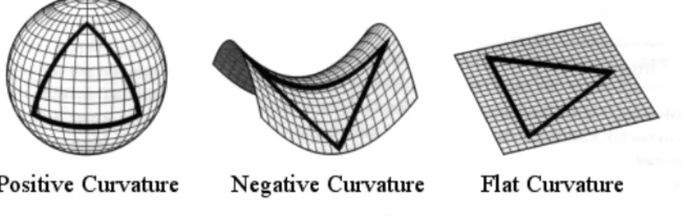
1.1 The cosmic microwave background as seen by the PLANCK satellite [1]. At the time of last scattering the universe was about 380 000 years old. The small temperature fluctuations correspond to regions of slightly different densities, which form the seeds of all future structure. 2 2.1 The three possible shapes of the FLRW universe; a spherical or closed

universe withk= +1, a hyperbolic or open universe withk=−1, or a flat universe withk= 0. Reproduced from [2]. . . 10 2.2 Conformal diagram for the standard FLRW cosmology illustrating

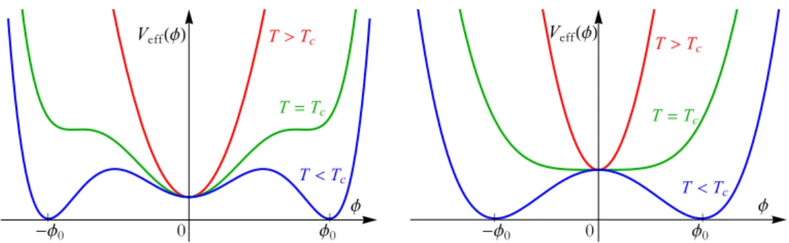
the horizon problem, based on [3]. The region of space which was in causal contact before recombination has a much smaller radius than the separation between two regions from which we receive CMB photons. 17 2.3 The shape of the effective potential depends on the temperature rel-

ative to the critical temperature. For high T > T_c, there is only one minimum at φ = 0. Once the temperature drops below the critical temperature, another minimum is established at φ0. Left: Old inflation is based on a first-order phase transition. The scalar field starts out atφ= 0, which becomes a false vacuum whenT < Tc. This phase of inflation lasts until the universe tunnels to the true vacuum at the global minimum φ₀. Right: The important phase in the new inflationary model happens after a second-order phase transition: when T < Tc, the field slowly rolls from zero to the minimum at φ0. . . 21 2.4 Conformal diagram for the inflationary cosmology illustrating the so-

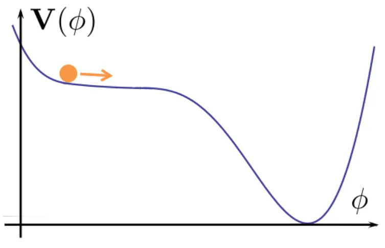
lution to the horizon problem, based on [3]. Causal contact between two regions separated by more than about two degrees in the CMB is achieved by increasing the amount of conformal time between the big bang, now atτ_i=−∞, and recombination atτ_rec, such that their past light cones overlap in the shaded region. The timeτ= 0becomes the time of reheating. . . 23 2.5 A simple inflationary model: on the plateau the potential is sufficiently

flat allowing the field to roll very slowly and inflation to occurs. . . . 25

(10)

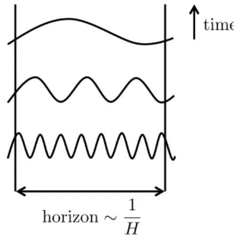
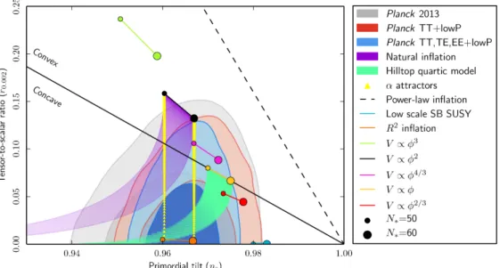
2.6 Perturbations exit the horizon during inflation: the horizon is almost constant while the fluctuations are stretched to such an extent that they exit the horizon when their wavelength becomes comparable to the horizon size. . . 31 2.7 Tensor-to-scalar ratior0.002versus scalar spectral indexnsfrom PLANCK

in combination with other data sets, compared to the theoretical predictions of selected inflationary models [4]. . . 37 2.8 The braneworld picture of our universe, based on [5]. Gravity can

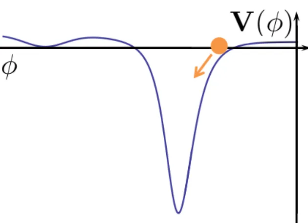
propagate in the whole spacetime while other forces and matter are localised on the (3 + 1)-dimensional branes. There is an attractive force between the two branes across the bulk spacetime that makes them collide at regular intervals. The collision corresponds to the big bang as seen from the brane. . . 40 2.9 A scalar field rolling down a steep, negative potential leads to an

ekpyrotic phase. . . 42 2.10 Perturbations exit the horizon during ekpyrosis: the fluctuations stay

almost constant while the horizon shrinks. . . 45 2.11 The decomposition into the adiabatic direction,σ, and the transverse

direction, s, is shown. Perturbations along the direction of the background trajectory are adiabatic/curvature perturbations, whereas perturbations orthogonal to the trajectory represent entropy/isocurvature perturbations. Based on [6]. . . 46 2.12 After a rotation in field space, the two-field ekpyrotic potential de-

composes into the adiabatic direction,σ, and the transverse tachyonic direction, s. The ekpyrotic scaling solution corresponds to motion along the ridge of the potential. Based on [7]. . . 47 4.1 After a rotation in field space, the two-field ekpyrotic potential can

be viewed as composed of an ekpyrotic direction (σ) and a transverse direction (s). The ekpyrotic scaling solution corresponds to motion along the adiabatic direction. Perturbations along the direction of the trajectory are adiabatic/curvature perturbations, while perturbations transverse to the trajectory are entropy/isocurvature perturbations. . 73 4.2 Left: The repulsive potentials (V1,2 withr= 0,1) given in Eq. (4.47).

Right: The field space trajectory in the repulsive potential V₁(r= 0). 83 4.3 The evolution of the fields (left), the field space metric and the scalar

(Ricci) curvature (right) during one e-fold of conversion (from t =

−275 to t = −47), plotted for the specific case with V₂(r= 1) = vh

(sinhx)⁻²+ (sinhx)⁻⁴i

, andΩ c= 1, b=d= ₁₀¹

= 1−₁₀¹ I0 1 10e^φ/2

, giving f_NL =−1.3 andg_NL =−544. . . 85

(11)

4.4 Non-Gaussianity plotted against different slopes of the scalar curvature (R˙) for different durations of the conversion (N =¹/2,²/3,³/4,1) for the repulsive potential V₂ with r = 1. The slope R˙ is varied by choosing different values for d=¹/10,¹/20,¹/50. Note that the magnitudes off_{N L}andg_{N L}are significantly reduced for smoother conversion processes. . . 85 4.5 Non-Gaussianity plotted against different slopes of the scalar curva-

ture (R˙) for different potentials (V1,2 with r = 0,1) for a conversion duration of one e-fold. The two r = 0 lines happen to be virtually coincident. Note that the values for fN L are clustered around zero, while the values for gN L are always appreciably negative. This is a characteristic feature of current ekpyrotic models. . . 86 4.6 The evolution of the fields, the field space metric and the scalar curva-

ture during one e-fold of conversion (fromt=−304tot=−46), plotted for the specific case withV₂(r= 1) =vh

(sinhx)⁻²+ (sinhx)⁻⁴i , and Ω b=d= ₅₀¹

= 1−₅₀¹e^φ/100, givingf_NL = 1.0and g_NL =−235. 87 4.7 Non-Gaussianity plotted against different field space metrics (Ω =

1−be^dφ/2 withb=d) for different durations of the conversion (N =

1/2,²/3,³/4,1) for the potentialV₂ withr = 0. Note that as in the case with a linearly decaying field space curvature, the magnitudes offN L

and gN L are significantly reduced for smoother conversion processes. 88 4.8 Non-Gaussianity plotted against different field space metrics (Ω =

1−be^dφ/2 with b=d) for different potentials (V1,2 with r = 0,1) for a conversion duration of one e-fold. . . 88 4.9 Non-Gaussianity plotted against different potentials (V_1,2 with r =

0,1) for a conversion duration of one e-fold for the minimal entropic mechanism. . . 90 5.1 Left: The original Jordan frame potential V_J is shown in blue, the

shifted potential UJ in dashed red. Right: The equation of state in Jordan frame, for the shifted potential. . . 98 5.2 Scalar field and scale factor in Jordan frame: the blue curves show

the transformed ekpyrotic scaling solution and the red dashed curves correspond to the field evolutions in the shifted potential. . . 99 5.3 The Einstein frame scalar potential used in the bounce model (5.32). 100 5.4 Left: Scalar field and scale factor for the bounce solution in Einstein

frame. Right: Parametric plot of the scalar field and scale factor in Einstein frame. This plot nicely illustrates the smoothness of the bounce.101

(12)

5.5 Full evolution of the scale factor for the transformed solution in Jor- dan frame. The conflationary phase lasts while the scalar field rolls up the potential towards Φ ∼10⁻⁹. During this period the scale factor increases by many orders of magnitude. During the exit of the conflationary phase the scale factor and scalar field undergo non-trivial evolution which is hard to see in the present figure and is shown in detail in Fig. 5.6 . . . 103 5.6 Left: Scalar field and scale factor for the transformed solution in Jor-

dan frame towards the end of the evolution. Right: Parametric plot of the scalar field and scale factor in Jordan frame. Note that initially the scalar field decreases in value very rapidly. Later on, as the scalar field stabilises, the scale factor goes through oscillations, but eventually increases monotonically. . . 103

(13)

Chapter 1

Introduction

When we look at the night sky we see an uncountable number of bright points – planets, stars and galaxies. And yet, the sky is much darker during the night than during the day. The overall relative darkness seems inconsistent with an infinite, static and eternal universe, as pointed out by astronomer Heinrich Wilhelm Olbers in the early 19th century: such a universe should be populated by an infinite number of stars and hence any line of sight from Earth would end in a star leading to an infinitely bright night sky. The resolution of the paradox is brought about by the big bang theory. Not only is the universe of finite age, but it also expands causing the energy of emitted starlight to be reduced via redshift.

Moreover, since the speed of light is finite as well, observing distant objects allows us to study the universe when it was much younger. The oldest photons we can detect originate from the time when, after the hot big bang, the expanding universe had cooled enough for neutral atoms to form and light to not be scattered anymore. This surface of last scattering is called the cosmic microwave background (CMB) as the photons that arrive at earth today have been redshifted to microwave wavelengths. Discovered by Arno A. Penzias and Robert W. Wilson [8] in 1965 as isotropic radiation with a uniform temperature of about 2.7 K, recent observations by the PLANCK satellite (see Fig.1.1) [9,4,10] show tiny temperature fluctuations with an amplitude of order one in 10⁵. The statistics of these small anisotropies constitutes the main source of information about the early universe. Hot spots correspond to overdense regions representing the seeds of all the structure we observe in the universe, like stars and galaxies.

Large-scale structure surveys, which observe the distribution of galaxies and galaxy clusters as the universe evolves in time, might lead to valuable new insights.

(14)

Figure 1.1: The cosmic microwave background as seen by the PLANCK satellite [1]. At the time of last scattering the universe was about 380 000 years old. The small temperature fluctuations correspond to regions of slightly different densities, which form the seeds of all future structure.

In the future, they might be able to rival the precision of the CMB maps, as our understanding of structure formation is continually improving [11]. While Einstein’s theory of gravity has been probed to extremely high precision in our solar system (see [12] for a review), it cannot account for the recently discovered acceleration of the universe [13]. We either have to assume a new form of energy density called dark energy that effectively acts as repulsive gravity, or gravity has to be modified on cosmological scales such that it allows for self-accelerating solutions [14].

Similarly to this late-time acceleration in the expansion of the universe a phase of inflation (see [3] for a review) during very early times has been postulated, yet at a much higher energy scale. A subsequent period of reheating would have slowed the expansion down while filling the universe with radiation and matter. Emerging from the big bang with typical initial conditions some regions of space supposedly have the properties required to undergo a period of inflation that smooths and flattens the universe, accounting for the homogeneity and isotropy of the CMB at the background level. Moreover, inflation provides an explanation for the small temperature anisotropies by stretching quantum fluctuations to cosmological distances. Simple scalar-field models of inflation lead to rather clear predictions for these perturbations: the so-called inflaton must roll down a very flat potential which implies that it is approximately a free field. This in turn leads to a spectrum of density perturba-

(15)

tions that is Gaussian to high accuracy, implying that both the bispectrum/3-point correlation function and trispectrum/4-point function are expected to be very small.

More complicated models can however be designed, involving multiple fields and/or higher-derivative kinetic terms, such that essentially all potential combinations of observations can be matched. One may hope that this uncomfortable fact could be circumvented if additional constraints on model building, arising from the combination with particle physics or eventually quantum gravity, become available. In the meantime, it is interesting to observe that simple inflationary models also typically predict primordial gravitational waves at observable levels, so that the current non-observation already starts to rule out a number of long-favoured models [4].

Experiments like the BICEP / KECK observatories at the south pole search for a primordial gravitational wave signal in the B-mode polarisation of the CMB [15]. A joint analysis with PLANCK showed that a significant contribution to the polarisation comes from galactic dust [16]. Measurements in the next few years operating at increased sensitivity will further constrain the origin of the observed signal.

From a theoretical point of view, single-field models of inflation present important challenges (see e.g. [17]): for one, inflation does not provide a complete history of the universe, and one may ask what happened before inflation and how the inflationary phase started. In fact, the initial conditions need to be very special: the scalar field has to start out at large potential energy with negligible initial velocity, everywhere within a region of the universe that is a billion times larger than the Planck scale. This requirement clashes somewhat with the motivation for inflation, which is to explain the specialness of the early universe in a dynamical fashion. A second complicating feature of (most) inflationary models is that they typically lead to the runaway behaviour of eternal inflation: large quantum fluctuations can mo- mentarily disrupt the inflationary dynamics and create an infinite number of causally disconnected pocket universes containing all possible values for the amplitude, the spectrum and the Gaussianity of the perturbations. In the absence of a measure (which the theory does not provide) the theory then loses all its predictive power and the naive predictions quoted above become questionable.

This situation suggests two possible approaches: the first is to try and under- stand the above-mentioned challenges better and to resolve them. On the other hand, we may look for alternative theories which might be able to explain the same cosmological data without however presenting us with such conceptual conundrums.

Evidently it is interesting to pursue both approaches – here, we will be concerned with the second approach.

(16)

The thesis is organised as follows: In the next chapter we follow the progress that has been made in describing the evolution of the universe, beginning with the old big bang theory based on Einstein’s theory of general relativity and Hubble’s observation that the universe expands. We show how inflation solves most of the puzzles con- nected with the hot big bang theory, most notably the horizon and flatness problem.

Moreover, we add quantum perturbations, which become the temperature fluctuations observed in the cosmic microwave background. Inflation contains problems of its own though, which we outline and take as motivation to investigate alternative theories such as the ekpyrotic / cyclic model. We then discuss how the big bang can be replaced with a bounce linking a contracting phase to the currently expanding phase in order to make these models viable.

Chapter3contains our main technical developments based on published work [18]

in collaboration with Jean-Luc Lehners. Employing the covariant formalism, we derive the evolution equations for two scalar fields with a non-minimal kinetic coupling up to third order in perturbation theory. Even though the scalar-field space is en- dowed with a non-trivial metric, the model does not contain higher-derivative kinetic terms. For this reason, only the non-Gaussianities of local form are relevant, and these can be calculated from the classical evolution on large scales. This will extend the existing treatment up to second order in perturbation theory by Renaux-Petel and Tasinato [19], as well as the existing development of third-order perturbation theory for trivial field space metrics [20]. These equations will be used to calculate the non-Gaussian corrections to the primordial density fluctuations in terms of the bispectrum and the trispectrum.

The results are applied to a new mechanism for generating ekpyrotic density perturbations in chapter4. The model we are interested in, non-minimal ekpyrosis, was first proposed by Qiu, Gao and Saridakis [21] and Li [22], and generalised in [23].

It contains two scalar fields, but only one has a steep negative potential, whereas the potential of the other is negligible or even precisely zero. The first field dominates the energy density and thus drives the ekpyrotic phase. In the non-minimally coupled entropic mechanism, nearly scale-invariant entropy perturbations are then generated by a field-dependent coupling between the two scalar field kinetic terms.

Subsequently, these entropy perturbations are converted into curvature perturbations. We show that this model leads to vanishing bi- and trispectrum during the ekpyrotic phase. Moreover, we investigate the effect of the conversion mechanism on both the bispectrum and trispectrum in detail. We show that the conversion process has a crucial impact on the final predictions for the bispectrum and trispectrum of

(17)

the curvature perturbations. In particular, we find that the conversion process must be very efficient in order for these models to be in agreement with current limits on the bispectrum parameterf_{N L}.Interestingly, such efficient conversions then lead to a non-trivial prediction for the trispectrum non-linearity parameter gN L, which is expected to be negative and of a magnitude of several hundred typically. The spectrum and bispectrum during the ekpyrotic phase were calculated in collaboration with Enno Mallwitz and Jean-Luc Lehners in [24], and the extension to the trispectrum and detailed analysis of the conversion were carried out together with Jean-Luc Lehners in [18].

Inflation and ekpyrosis share a number of features: they are the only dynamical mechanisms known to smoothen the universe’s curvature (both the homogeneous part and the anisotropies) [25, 26]. They can also amplify scalar quantum fluctuations into classical curvature perturbations which may form the seeds for all the large-scale structure in the universe today [27,28]. Moreover, they can explain how space and time became classical in the first place [29]. With a number of assumptions, in both frameworks models can be constructed that agree well with current cosmological observations, see e.g. [30,31]. But in other ways, the two models are really quite different: inflation corresponds to accelerated expansion and requires a significant negative pressure, while ekpyrosis corresponds to slow contraction in the presence of a large positive pressure. Inflation typically leads to eternal inflation and the associated ambiguities about its actual predictions [17], while ekpyrosis requires a null energy violating (or a classically singular) bounce into the expanding phase of the universe [32]. In chapter5we introduce the idea of conflation, which corresponds to a phase of accelerated expansion in a scalar-tensor theory of gravity and which combines elements from both inflation and ekpyrosis. In the conflationary model, the universe is rendered smooth by a phase of accelerated expansion, like in inflation.

However, the potential is negative, and adiabatic scalar and tensor fluctuations are not amplified, just as for ekpyrosis. Hence eternal inflation and the associated infinities are avoided. As we will show, one can obtain nearly scale-invariant curvature perturbations by adding a second scalar field and employing an entropic mechanism analogous to the one used in ekpyrotic models. This chapter is based on work [33]

done in collaboration with Enno Mallwitz and Jean-Luc Lehners.

(18)

Chapter 2

The early universe

In this chapter we will set the scene for the following ones in terms of the structure of the theories we study as well as notation. We describe the historical development of early universe cosmology, including the hot big bang model as well as the inflationary theory designed to resolve the puzzles that arose with the former. We then discuss problems of inflation which motivate the investigation of alternative theories of the early universe. We work in reduced Planck units, c=~= 1 and 8πG=M_Pl⁻² = 1, which eliminates the factor 8πG from the Einstein field equations, unless stated otherwise.

2.1 Friedmann-Lemaître-Robertson-Walker cosmology

The fact that the universe expands was probably the most important discovery in cosmology in the last century. In 1917 Albert Einstein [34,35] realised that according to general relativity the universe had to either expand or contract. However, to match the absence of observational evidence for any form of dynamical evolution of the universe, he added a positive cosmological constant¹, even though a static universe is not a stable solution. Alexander A. Friedmann [36,37] then found the full set of solutions for models of the universe with positive, zero and negative curvature. In 1927 George Lemaître [38,39] was the first to take the implications of an expanding universe seriously. He concluded that the universe must have had an origin, which he later called the “primeval atom”. In 1929 Edwin P. Hubble [40] discovered that

1In later years Einstein declared the introduction of the cosmological constant his “biggest blun- der”. As a matter of fact, there is no a priori reason for the constant to vanish – the constant can indeed be used to model dark energy. Einstein’s mistake consisted in overlooking the instability of his solution.

(19)

the further away a galaxy is from us, the more redshifted it is. This proportionality between the recession speed of galaxies and their distance from us is called Hubble’s law, and admits the interpretation that the universe does indeed expand. Moreover, in the 1940s George Gamow [41,42] laid the foundation for our present understanding of hot big bang nucleosynthesis. He explained the observed relative abundance of light elements like helium, deuterium and lithium by taking into account how the temperature of the universe decreased due to its expansion after starting out in a very hot and dense state. Lastly, in 1965 Arno A. Penzias and Robert W. Wilson [8] discovered the cosmic microwave background, the afterglow of the big bang. The isotropic black body radiation (today at about 2.73K) was emitted around 380,000 years after the big bang from the so-called “surface of last scattering” when the universe had cooled enough to form neutral atoms and photons decoupled from matter.

Over the last decades these observations have been confirmed, and more and more detail of the CMB and large scale structure (LSS) has been obtained, establishing the hot Big Bang as the preferred model of the universe². However, there are certain issues which make it unlikely that this is a complete model – they will be discussed in section2.2.

2.1.1 The Friedmann-Lemaître-Robertson-Walker metric

According to the Cosmological Principle (CP) the universe is homogeneous and isotropic on large scales. Homogeneity means that, if the evolution of the universe is represented as a time-ordered sequence of 3D space-like hypersurfaces, the physical conditions are the same at each point of a given hypersurface. For a spacetime to be isotropic, the physical conditions have to be identical in all directions when viewed from a given point on the hypersurface, i.e. there are no preferred directions in space.

The CP is a generalisation of the Copernican Principle at the cosmological level. The latter assumes that we do not occupy a privileged position in our universe. Since the universe is isotropic around us, it should thus be isotropic everywhere, automatically implying homogeneity³.

On scales smaller than about 100Mpc⁴, the CP is no longer valid. Clearly, the

2According to the current understanding of the evolution of our universe, there are two dark components that have to be included: (cold) Dark Matter and Dark Energy, potentially in the form of the cosmological constantΛ. The preferred model of the universe is thus referred to as ΛCDM – see section2.1.2.

3Note that isotropy at every spacetime point implies homogeneity but not vice versa.

4One parsec (pc), an abbreviation of theparallax of one arcsecond, is the distance at which one

(20)

centre of the sun or our galaxy is very different from interstellar or intergalactic space, respectively. The largest known structures are galaxy filaments that consist of gravitationally bound galaxies and form the boundaries between large voids in the universe. Beyond those structures it has been confirmed by modern observations that local variations in matter are averaged out, and we can assume that the CP is applicable. Not only are radio galaxies randomly distributed across the entire sky, the distribution of the observed redshift in the spectra of distant galaxies is also isotropic, implying a uniform Hubble flow, i.e. expansion of the universe, in all directions. In addition to observations from LSS, the most important source is the CMB; temperature anisotropies at the time of last scattering are only of the order of one part in10⁵ ⁵, as shown for the first time by the COsmic Background Explorer (COBE) satellite in 1992 [43].

In general relativity, the CP implies that we can foliate the 4D manifold of the universe as R×Σ, where R represents the time direction and Σ is a maximally symmetric 3-space – the universe is homogeneous and isotropic in space, but not in time. The metric can thus be taken to be of the form

ds² =−dt²+a²(t)γij(x)dxⁱdx^j, (2.1) wheretis a time-like coordinate, labelling cosmological events in the 3-surfaceΣ(x), and the metricγij is maximally symmetric inΣ. The scale factora(t)represents the relative size of spatial sections ofΣ at timet. Note that g_0i= 0 due to the isotropy requirement, as it would otherwise introduce a preferred direction.

Isotropy further implies that the maximally symmetric spatial metric d`² = γ_ij(x)dxⁱdx^j has to be spherically symmetric, and can therefore be written as

d`²=e^2β(r)dr²+r² dθ²+sin²θdφ²

, (2.2)

where the form of the functiongrr(r) =e^2β(r) has been chosen for convenience. The

astronomical unit (the average distance between the Earth and the sun, 150 million kilometres) subtends an angle of one arcsecond.100Mpc equals about3.26·10⁸ light-years, or about3.08·10²¹ km in length.

5Actually, due to the peculiar motion of the Earth w.r.t. the cosmological rest frame of the CMB (around the sun, around the galactic centre, within the motion of our galaxy cluster), there is a dipole anisotropy ofδT /T ∼10⁻³, which has to be subtracted off.

(21)

components of the Ricci tensor for this metric are

(3)Rrr = 2 r∂rβ

(3)R_θθ =e^−2β(r∂_rβ−1) + 1

(3)Rφφ =h

e^−2β(r∂rβ−1) + 1i sin²θ

(2.3)

Moreover, maximally symmetric metrics obey

(3)Rikjl =k(γijγkl−γilγkj), (2.4) wherek is a constant due to homogeneity. The Ricci tensor is then given by

(3)Rij = 2kγij. (2.5)

Equating the two expressions for the Ricci tensor, (2.3) with (2.5), we can solve for β(r), obtaining

β =−1

2ln 1−kr²

. (2.6)

Thus, the spacetime metric becomes ds² =−dt²+a²(t)

dr²

1−kr² +r² dθ²+ sin²θdφ²

, (2.7)

which is the famous Friedmann-Lemaître-Robertson-Walker metric (FLRW). Note that this metric is invariant under the redefinition

k→ k

|k|, r→rp

|k|, a→ a

p|k|, (2.8)

so that the only relevant parameter is k/|k|. There are three cases of interest: a closed universe, with constant positive curvature,k= +1; a flat universe of vanishing spatial curvature, k = 0; and an open universe, with constant negative curvature, k=−1(see Fig. 2.1).

2.1.2 The Einstein equations

As outlined in the beginning of the section, modern cosmology began as a quan- titative science with the advent of Einstein’s general relativity. He showed that gravitation is a distortion of the structure of spacetime by matter, affecting the

(22)

Figure 2.1: The three possible shapes of the FLRW universe; a spherical or closed universe withk= +1, a hyperbolic or open universe withk=−1, or a flat universe withk= 0. Reproduced from [2].

inertial motion of other matter. The Einstein field equations relate the spacetime geometry, given in terms of the Einstein tensorGµν, to the energy density in terms of the stress-energy tensorT_µν,

G_µν ≡R_µν −1

2g_µνR= 8πG T_µν, (2.9) where we have temporarily reinserted the factor8πG.

In addition to the FLRW metric from the last section, which determines the left-hand side, we need to model the matter and energy in the universe. The most general matter fluid consistent with the CP is a perfect fluid, where an observer comoving with the fluid would see the universe around it as spatially isotropic. The energy-momentum tensor associated with a perfect fluid can be written as

T^µν =pg^µν+ (p+ρ)u^µu^ν, (2.10) wherep(t)andρ(t)are the pressure and energy density of the fluid, respectively, and u^µ is the comoving four-velocity, satisfyinguµu^µ=−1. With the four-velocity for a fluid at rest in comoving coordinates given byu^µ= (1,0,0,0), the energy-momentum tensor becomes

T_ν^µ=diag(−ρ(t), p(t), p(t), p(t)). (2.11) The µ=ν= 0 component of the Einstein equations (2.9) and its combination with

(23)

theµ=ν=icomponent then lead to the so-called Friedmann equations 3

a˙ a

2

=ρ−3k

a², (2.12)

3¨a

a =−ρ+ 3p

2 . (2.13)

In order to find explicit solutions, it is necessary to choose an equation of state, a relationship between energy density and pressure. The most relevant fluids in cosmology obey the simple equation of state

p=wρ, (2.14)

wherew is a constant.

The ν = 0 component of the covariant conservation of the energy-momentum tensor, Tν;µ^µ = 0, gives

T_0;µ^µ = 0 =−ρ˙−3a˙

a(ρ+p). (2.15)

Substituting the expression for the equation of state parameter w from (2.14), we obtain the continuity equation

˙ ρ

ρ =−3a˙

a(1 +w), (2.16)

which can be integrated to give

ρ∝a^−3(1+w). (2.17)

There are several fluids which are of particular interest in cosmology: Dust is colli- sionless, nonrelativistic matter, whose equation of state obeys wm = 0. Hence from (2.17), the energy density in matter, which is proportional to the number density of particles, falls off asρ(matter)∝a⁻³ with the expansion of the universe. Examples include ordinary stars and galaxies as well as dark matter, for which the pressure is negligible in comparison with the energy density.

Radiation has an equation of state given bywr= 1/3, and is associated with rel- ativistic degrees of freedom, i.e. not only photons, but also nearly massless particles like for example neutrinos. In an expanding universe the energy density of radiation decays as ρ(radiation)∝a⁻⁴: in addition to the decrease in number density, individual photons also lose energy in proportion toa⁻¹ as they redshift.

(24)

Einstein’s cosmological constant can be given in terms of the energy-momentum tensor as T_µν^vac = −Λg_µν, and is perhaps associated with the energy of the vacuum itself⁶. The vacuum energy density has an equation of state w_Λ =−1, and remains constant with the expansion of the universe, providing a possible explanation for the observed late time accelerated expansion of the universe due to dark energy.

The energy density of anisotropies in the curvature of the universe can be shown to scale as ρ(anisotropies)∝a⁻⁶ [5]: We consider a metric of the Kasner type (a special case of the Bianchi I metric) with negligible initial curvature,

ds²=−dt²+a(t)²X

i

e^2βⁱ^(t)dxⁱdxi with X

i

βi= 0. (2.18) The Friedmann equations become

H² = 1 3ρ+1

6 X

i

β˙_i², (2.19)

H˙ = −1

2(ρ+p)−1 2

X

i

β˙_i², (2.20)

where we have introduced the Hubble parameter, H(t) = ^a_a^˙. Together with the condition on the Kasner exponents in (2.18) they imply

β¨_i+ 3Hβ˙_i= 0, (2.21)

which has the growing mode solution β˙i ∝ a⁻³. Hence the energy density in the anisotropies scales as ¹₂P

iβ˙_i² ∝a⁻⁶, where we will denote the constant of proportionality byσ².

The first Friedmann equation (2.12) can then be rewritten in the following form 3H² = Λ−3k

a² +ρm

a³ + ρr

a⁴ +σ²

a⁶ +· · ·+ ρφ

a^3(1+w^φ⁾, (2.22)

where we have added the scaling for a scalar field φ, which will become important later. We can infer the energy density content of the universe by combining measurements of the CMB, LSS and Type Ia supernovae. In terms of the fraction of the total energy density,Ωi,0 ≡ρi,0/3H², it consists of radiation (Ωr,0 ≈ O(10⁻⁵)), baryonic and dark matter (Ω_m,0≈0.31), and dark energy (Ω_Λ,0 ≈0.69), which can

6A naive estimate of the contribution of the energy associated with quantum vacuum fluctuations over-estimates the vacuum energy relative to the observational constraint by more than∼120orders of magnitude [44].

(25)

be modelled byΛif it is constant. Nearly all the energy density today is contained in the latter two, such that this parametrisation of the standard big bang cosmology is called theΛCDM (Lambda cold dark matter) model. The Friedmann equation then shows how the different components scale with the expansion of the universe due to their dependence on a. Radiation dominated during early times, before matter and finally dark energy took over. The first two imply decelerated expansion of the universe, with the scale factor going like t^1/2 and t^2/3, respectively, whereas dark energy domination implies accelerated expansion.

2.2 Puzzles

Due to its successes in describing our universe the ΛCDM model is also referred to as the standard model of cosmology. It not only predicts the existence of the cosmic microwave background, but also the observed abundances of hydrogen, helium and lithium in interstellar gas produced during primordial nucleosynthesis. Moreover, the cosmological parameters (including dark energy) are such that the age of the universe comes out larger than the age of the oldest objects we can observe, like stars in globular clusters. Dark matter plays a key role in structure formation since it begins to collapse into a complex network of dark matter halos well before ordinary matter, which is impeded by radiation pressure. Without dark matter, the epoch of galaxy formation would occur substantially later in the universe than is observed.

Despite these achievements, there are some aspects of the model which require further consideration. From precise measurements of the CMB we know that the early universe was extraordinarily simple: not only approximately flat, homogeneous and isotropic, but also containing nearly scale-invariant and Gaussian density fluctuations. A major goal of cosmology is to find a convincing explanation for this initial state. For the standard model of cosmology to provide a consistent theory to explain the state of the observable universe, we have to assume very particular initial conditions whose origin is not explained. Instead of putting them in by hand, we want to explain dynamically why the universe looks the way it does. The specialness of the initial state can be quantified in terms of the horizon problem and the flatness problem, which we discuss in more detail in sections 2.2.1and 2.2.2, respectively.

Another problem is related to the very high temperatures in the early universe.

Grand unified theories (GUTs) propose that at high temperatures (above TGUT ∼ 10¹⁵GeV) the electromagnetic, the weak and the strong interactions are not actually fundamental forces but arise due to spontaneous symmetry breaking (SSB) from

(26)

a single gauge theory. As the temperature drops through the GUT threshold, a phase transition associated with SSB occurs. Depending on the properties of the symmetry breaking, the phase transition can produce topological defects such as magnetic monopoles, strings, domain walls or textures via the Kibble mechanism [45, 46]. Different regions of the universe fall into different minima in the set of possible states. Topological defects are then precisely the “boundaries” between these regions with different choices of minima. Their formation is an inevitable consequence of the fact that different regions cannot agree on their choices since the correlation length cannot be larger than causality would allow, i.e. it must be at least as big as the horizon size. Accordingly, in the case of the GUT phase transition, at least one magnetic monopole should be produced per horizon volume (determined at the time when the symmetry breaking took place) [47,48]. They should have persisted until the present day, to such an extent that the resulting monopole number density would be some ten orders of magnitude bigger than the critical density of the universe [49, 50]. Not only is that not the case, but all searches of them have failed, placing tight limits on the density of relic magnetic monopoles in the universe [51].

The observation of the expansion of the universe brought about another puzzle, namely the big bang singularity. Extrapolating backwards in time, the density and temperature of matter as well as the spacetime curvature diverge and general relativity predicts its own breakdown. According to the singularity theorems of Hawking and Penrose [52] such a singularity, at which time and space are supposed to begin, is unavoidable. The theorems are based on certain assumptions that translate into the condition that the null energy condition has to be satisfied in a flat FLRW universe – the known matter and energy density content of the universe including dark energy fulfil this condition. A full theory of quantum gravity, which remains to be found, is generally expected to resolve the singularity and provide a physical description of the big bang event.

2.2.1 Horizon problem

In this subsection we will show that the fact that the universe is homogeneous and isotropic on large scales constitutes a problem. When we evolve the universe back in time using GR, the finiteness of the speed of light implies that there are regions in the CMB that have never been in causal contact since the big bang. Yet, they have nearly the same temperature. It is basically a strong initial conditions problem: the big bang must have occurred simultaneously in at least10⁵ adjacent regions – it did

(27)

not originate from a single point.

The problem can be studied in some more detail by looking at the FLRW metric (2.7) for radial propagation of light in a flat universe, with k= dθ= dφ= 0, which simplifies to

ds²=−dt²+a(t)²dr²=a(τ)²

−dτ²+ dr²

, (2.23)

where we have introduced the conformal timeτ via the relation dτ = dt

a(t). (2.24)

For null geodesics the line element vanishes: ds² = 0. We can thus integrate (2.23) to give the maximal distance a photon can travel between an initial time t_i and a later timet > ti

∆r= ∆τ =τ −τi = Z t

ti

dt

a(t), (2.25)

which is equal to the amount of conformal time elapsed during the interval ∆t = t−ti. The so-calledcomoving particle horizon,∆rmax, is then defined as the greatest comoving distance from which an observer at time t will be able to receive signals travelling at the speed of light since the big bang started, defined formally by the initial singularity atai=a(ti= 0) = 0. In other words, causal influences have to come from within this region.

The integral (2.25) can be rewritten in terms of the comoving Hubble radius (aH)⁻¹ as

∆r = Z dt

a(t) = Z

(aH)⁻¹d lna. (2.26)

For a universe dominated by a perfect fluid withp=wρ, as described in the previous subsection, the scale factor goes like

a∼t^3(1+w)² , (2.27)

which can be obtained from integrating the Friedmann equation (2.12) together with the continuity equation (2.17). Thus, the comoving Hubble radius evolves as

(aH)⁻¹ ∼a¹²^(1+3w). (2.28)

(28)

Performing the integral in (2.26), we obtain τ ∼ 2

(1 + 3w)a¹²^(1+3w). (2.29) All familiar matter sources satisfy the strong energy condition (SEC), 1 + 3w > 0. The comoving horizon (2.25) is thus finite as τi=τ(ai= 0) = 0:

∆rmax=τ−0∼a(t)¹²^(1+3w), for w >−1

3. (2.30)

We can show that this implies that most spots in the CMB have non-overlapping past light-cones and hence never were in causal contact by calculating the angle subtended by a causal patch in the CMB. The horizon length at recombination corresponds to an angular size on the sky of

θ_{hor, rec} = ∆r_max(z_rec)

d_A(z_rec) , (2.31)

which is the ratio of the comoving particle horizon at recombination and the comoving angular diameter distance from us (at redshiftz0= 0) to recombination (zrec≈1100).⁷ The cosmological redshift z of a source observed from Earth (at a₀= 1) is defined via

a= (1 +z)⁻¹. (2.32)

Thus, the comoving particle horizon (2.26) at the time of last scattering becomes

∆r_max(z_rec) = Z arec

ai=0

da a²H

MD≈

Z (1+zrec)⁻¹ 0

da

a^1/2H₀ = 2 H0

(1 +z_rec)^−1/2, (2.33) where the main contribution to the integral comes from times in which pressureless matter dominates (MD) the Hubble expansion rate H ^MD= _3t² = H₀a^−3/2 since a∼ t^2/3, which can be inferred from the Friedmann equation (2.22).

The comoving angular diameter distance is defined as the ratio of the assumed comoving size of an object,D, and the measured angular diameter,∆θ, and can be determined from the angular part of the metric (2.7) withdt= dr= dφ= 0and hence aD=ar∆θ, such that

dA= D

∆θ =r, (2.34)

7Notice that the definition of the subtended angle does not change if instead we used the proper particle horizon and proper angular diameter distance, as the factors ofawould cancel each other.

(29)

⌧

₀

⌧

₀

⌧

_rec

⌧

_rec

⌧

_i

= 0

⌧

_i

= 0

Figure 2.2: Conformal diagram for the standard FLRW cosmology illustrating the horizon problem, based on [3]. The region of space which was in causal contact before recombination has a much smaller radius than the separation between two regions from which we receive CMB photons.

where we have to integrate from the scale factor at recombination, a(zrec), to the one today, a₀. Hence,

d_A(z_rec) ^MD≈

Z a0=1 (1+zrec)⁻¹

da

a^1/2H₀ = 2 H0

h1−(1 +z_rec)^−1/2i _z_rec₁

≈ 2 H0

, (2.35) where we have again assumed matter domination.

We finally obtain the angular size on the sky of the horizon length at recombination⁸:

θhor, rec= ∆rmax(zrec)

d_A(z_rec) ≈(1 +zrec)^−1/2 ≈0.03≈1.7^◦. (2.36) We conclude that regions in the CMB separated by more than about two degrees have never been in causal contact. Nevertheless, their temperature is the same up to one part in ten thousand, giving rise to the horizon problem.

2.2.2 Flatness problem

From the scaling of the different energy density components with the scale factor in the Friedmann equation (2.22), we can deduce that after a phase of radiation-

8The actual value is a bit smaller,θhor, rec≈1.2^◦, as the universe has not been matter-dominated throughout its whole evolution.

(30)

and matter-domination, the curvature should come to dominate in an expanding universe. Dividing the Friedmann equation by the critical density ρ_crit = 3H², we can define the density parametersΩi as

Ωi ≡ ρi

ρcrit

, (2.37)

and thus Eq. (2.22) becomes

1 = Ω_Λ+ Ω_k+ Ω_m+ Ω_r+ Ω_σ2+. . . . (2.38) However, from observations we know that our universe is very close to spatially flat today, i.e. the energy density in curvature is in fact negligible, [9]

Ωk≡ −k (aH)²

t0

= 0.000±0.005 (2σ). (2.39) In other words, the energy density in dark energy, baryonic and dark matter, radiation and anisotropies – where the contribution from the latter two is also insignificant – approximately adds up to unity,

1≈Ω_Λ+ Ω_m. (2.40)

Assuming that the expansion is dominated by some form of matter with equation of statew, the change in the curvature density parameter is given by

˙Ωk=HΩ_k(1 + 3w) Ω_k,N =±Ω_k(1 + 3w), (2.41) where we have used (2.27), allowing both for the universe to expand (with H >0) and to contract (withH <0). We have introduced the number of e-folds of evolution of the universe,N, defined via

dN = d lna=Hdt, (2.42)

where the dependence on the Hubble rate explains the appearance of the minus sign in the second equation of (2.41). For matter satisfying the SEC, i.e.w >−1/3, the solution Ωk = 0 is then an unstable point in an expanding universe – ifΩk >0 at some point, it keeps growing, whereas if Ω_k <0, it keeps decreasing. On the other hand, any matter satisfying the SEC in a contracting universe will drive the universe to spatial flatnessΩk→0.

(31)

Assuming we can simply extrapolate back to the Planck time, the curvature density would go like

Ω_k,Pl

Ω_k,0 = (aH)²₀

(aH)²_Pl. (2.43)

For a rough estimate we can assume radiation-domination as most of the e-folds of evolution of the universe occur during that phase. From the scaling of awith time (2.27) and w_r = 1/3, we havea∝t^1/2 and hence(aH)²∝t⁻¹. Thus,

Ω_k,Pl Ωk,0

= t_Pl

t0 ∼10⁻⁶⁰. (2.44)

Not only is the curvature observed today very close to zero (2.39), at the Planck time, it must have been 60 orders of magnitude smaller still! Even though we might not be able to trust the extrapolation all the way back to the Planck time, this simple estimate shows that the universe must have been extremely flat at early times.

2.3 Inflation

In 1979 Robert H. Dicke and Phillip J. E. Peebles [53] were the first to draw real attention to the puzzles described in the last section, in particular the flatness problem. In the same year, Robert Brout, Francois Englert and Edgard Gunzig proposed a model in which the matter emerging from quantum fluctuations had a large negative pressure, giving rise to “an open universe that closely resembles a de Sitter space” [54]. They were interested in this inflationary phase as a means to create a universe out of nothing, however, and not as a way to solve the hot big bang problems. By semi-classically incorporating quantum corrections to general relativity, Alexei A. Starobinsky [55,56] found a class of cosmological solutions that begin with a de Sitter phase, evolve through an oscillatory phase, and eventually make a transition into the standard FLRW expanding solution. The backreaction generi- cally leads to R²-corrections to the Einstein-Hilbert action. Moreover, he predicted a large gravitational wave amplitude when compared to a radiation-dominated phase – the amplitude is small compared to other, subsequent inflationary models. His approach required choosing a special state for the early universe, namely the maximally symmetric de Sitter spacetime, rather than an arbitrary initial state. In that sense Starobinsky’s original motivation was quite different from the goals of inflationary cosmology.

In 1980, two papers were published that addressed the horizon problem: Kat-

(32)

suhiko Sato [57] suggested that a phase of exponential expansion could increase the region between domain walls to a size larger than the observable universe, making them unobservable today. Furthermore, Demosthenes Kazanas [58] proposed that during a phase transition in the early universe the expansion can be exponential, potentially accounting for the observed isotropy of the universe if the phase lasts long enough.

In his seminal paper [25], Alan H. Guth was very clear in his motivation to solve the horizon and flatness problems, and finally coined the term inflation. He proposed that the universe underwent a phase of accelerated expansion during a false vacuum phase before decaying to the true vacuum via a bubble nucleation. The model, now called “old inflation”, suffers from agraceful exitproblem though. All the energy after the nucleation of a bubble is transferred to its walls, and can only be thermalised through many collisions with other bubble walls. However, if inflation lasts long enough to solve the initial conditions problems, collisions between bubbles become exceedingly rare. Thus, in any one causal patch too little reheating takes place, leading to large inhomogeneities in contradiction with observations.

To overcome the graceful exit problem Andrei D. Linde [59] and independently Andreas Albrecht and Paul J. Steinhardt [60] effectively replaced the first-order phase transition with a second-order one – see Fig 2.3. Both models of the GUT phase transition were based on a Coleman-Weinberg [61] effective potential for the Higgs field.

Expressed in terms of a scalar field (called the inflaton) in a symmetry-breaking potential below the critical temperature T < Tc, old inflation takes place while the field sits in the local, metastable minimum at φ = 0 – the false vacuum – before tunnelling through the barrier to the true vacuum at φ₀. In “new inflation” the crucial ultra-rapid expansion phase no longer takes place while the field sits at the now unstable equilibrium at φ = 0, but during the time that it slowly rolls on an extremely flat effective potential towards the symmetry-breaking minimum φ₀. Reheating takes place once the potential energy stored in the scalar field is converted to radiation when the field starts rolling faster and eventually oscillates around the minimum.

These models are also called small-field inflationary models as the inflaton is displaced by less than a Planck mass, and they face several issues of their own. It becomes necessary to severely fine-tune the shape of the Coleman-Weinberg type potential such that there is a very flat plateau near φ = 0 in order to satisfy the slow-roll conditions. A further problem for many slow-field models is that the slow-

(33)

Φ

0 Φ₀

-Φ₀

V_effHΦL _T_>_T_c

T=Tc

T<Tc

È È

Φ

0 Φ₀

-Φ₀

V_effHΦL

T>Tc

T=Tc

T<Tc È È

Figure 2.3: The shape of the effective potential depends on the temperature relative to the critical temperature. For high T > Tc, there is only one minimum at φ= 0.

Once the temperature drops below the critical temperature, another minimum is established atφ₀. Left: Old inflation is based on a first-order phase transition. The scalar field starts out at φ= 0, which becomes a false vacuum when T < Tc. This phase of inflation lasts until the universe tunnels to the true vacuum at the global minimum φ₀. Right: The important phase in the new inflationary model happens after a second-order phase transition: when T < Tc, the field slowly rolls from zero to the minimum at φ0.

roll trajectory is not an attractor in phase space; the initial field velocity must be constrained to be very small. Furthermore, in order to obtain a sufficiently small amplitude of density perturbations, the inflaton field must have a very small coupling constant. However, this implies that the inflaton could not be in thermal equilibrium with other matter fields. In the absence of thermal equilibrium, the phase space of initial conditions is much larger for large values of the field, i.e. it is unlikely that the scalar field would begin rolling close to its symmetric point at φ= 0.

In 1983 Linde proposed the first large-field model, which he called “chaotic inflation” [62]. He abandoned the idea that the universe was in a state of thermal equilibrium from the very beginning, but considered a universe that initially consisted of many domains with a chaotically distributed scalar field. Different scalar field potentials are then possible, where it is assumed that inflation takes place while the scalar field slowly rolls towards the origin from large values of φ & M_Pl. Do- mains in which the scalar field is too small never inflate, whereas those domains that originally contained large field values in the slow-roll regime of the potential do and hence make up the main contribution to the total volume of the universe.

If the inflationary phase lasts for long enough, it can solve the horizon, flatness and magnetic monopole problems by smoothing out inhomogeneities, anisotropies and the curvature of space, and diluting topological defects. However, in addition to the background the CMB contains small temperature fluctuations – the seeds for