Capacities and Gap analysis

Last updated: 06 April 2017

This project has received funding from the European Union’s Horizon 2020 research and innovation programme under grant agreement n^o 633211.

Project AtlantOS – 633211 Deliverable number D.1.3

Deliverable title

Capacities and Gap analysis

Description Analysis of the capacities and gaps of the present Atlantic Ocean Observing System.

Work Package number WP1

Work Package title Observing System and requirements and design studies Lead beneficiary IOC/UNESCO

Lead authors Erik Buch, Artur Palacz, Johannes Karstensen, Vicente Fernandez, Mark Dickey-Collas, Debora Borges

Contributors Michael Ott, Isabel Sousa Pinto, Albert Fischer, Maciej Telszewski, Siv Lauvset

Submission data 3 April 2017

Due date Month 24 (March 2017) Comments

2

3

List of content

List of Figures 4

List of Tables 6

Executive summary 7

1 Introduction 8

2 Phenomena 10

2.1 Physical Phenomena 10

2.1.1 Overview map areas of selected physical Phenomena in the Atlantic 15

2.2 Biogeochemical Phenomena 15

2.2.1 Maps of biogeochemical phenomena hot spots 32

2.3 Biological Phenomena 32

2.3.1 Overview map areas of selected Phenomena in the Atlantic 37

3 Essential Ocean Variables 40

3.1 Physical EOVs 41

3.2 Biogeochemical EOVs 42

3.3 Biological EOVs 43

3.3.1 EOVs and indicator development within the Regionals Seas Conventions 50

4 Observing elements/platforms/techniques 52

4.1 Physics 55

4.2 Biogeochemistry 56

4.3 Biology 60

5 Estimate of existing observation capacity in Atlantic per EOV and platform 62

5.1 Sources of information: European and international level 62

5.2 Observing capacity by platform and EOV 68

5.2.1 Physics 69

5.2.2 Biogeochemistry 80

5.2.3 Biology 86

6 Gaps 87

6.1 Examples of gaps in the biogeochemical observing system in the Atlantic 88

6.2 Examples from existing gap identification 93

6.2.1 Climate 93

6.2.2 WMO Rolling Requirement Review 95

7 Summary and conclusions 98

8 References 100

4

List of Figures

Figure 1-1. Stages of the value chain described in D1.1 (Initial AtlantOS Requirements Report) and current

deliverable (D1.3). ... 9

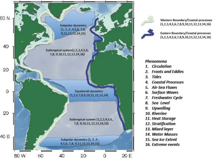
Figure 2-1. A conceptual map roughly delineating potential hot spots for observing the physical phenomena. Other areas not included on this map could be equally important to study given phenomena on a regional basis. Phenomena are likely to operate on different spatio-temporal scales in different regions. ... 15

Figure 2-2 Global full water column inventories of Cant. From Khatiwala et al. (2013). ... 24

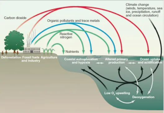
Figure 2-3. Schematic of human impacts on ocean biogeochemistry either directly via fluxes of material into the ocean (coloured arrows) or indirectly via climate change and altered ocean circulation (black arrows). Source: Doney (2010). ... 29

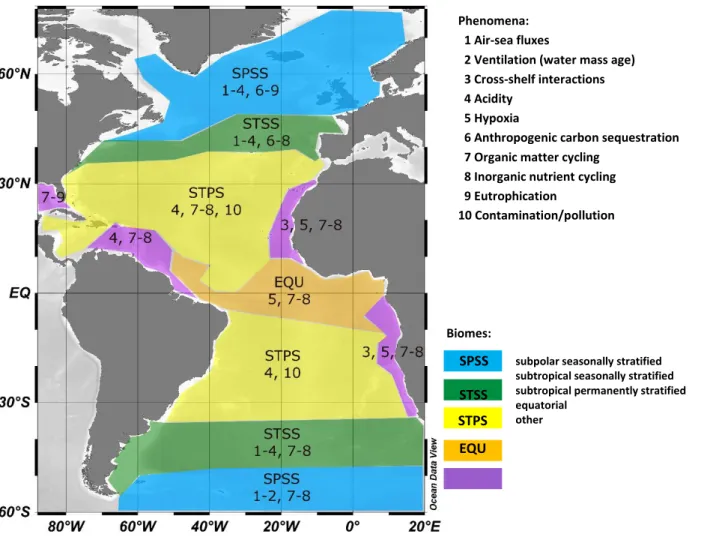
Figure 2-4. A conceptual map roughly delineating potential hot spots for observing the 10 biogeochemical phenomena considered in this report, distributed with respect to areas of mean annual biomes adapted from Fay & McKinley (2014). Other areas not included on this map could be equally important to study given phenomena on a regional basis. Phenomena are likely to operate on different spatio-temporal scales when compared across the hot spots. Mean biome map created from mean climatologies of maximum mixed layer depth, sea surface temperature, summer Chl-a concentration, and maximum ice fraction. Blue: subpolar seasonally stratified biome (SPSS); green: subtropical seasonally stratified biome (STSS); yellow: subtropical permanently stratified biome (STPS); orange: equatorial biome (EQU); purple: other ocean areas that do not fit the criteria for any of the above biomes. ... 32

Figure 2-5. Location of EBSAs in the Atlantic Ocean. Source: https://www.cbd.int/ebsa/ ... 38

Figure 2-6. Current NEAFC vulnerable marine ecosystems, closed to bottom fishing. ... 39

Figure 2-7. Current NAFO vulnerable marine ecosystems closed to bottom trawl fishing. ... 39

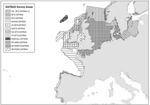
Figure 3-1. Examples of trawl surveys that target fish on the European continental shelf. ... 46

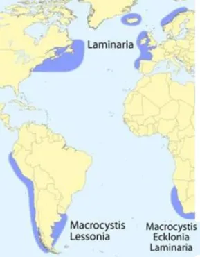
Figure 3-2. Kelp forests (part of macroalgal canopy EOV) distribution in the Atlantic. Source: Steneck et al (2002). ... 48

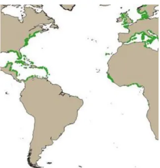
Figure 3-3. Seagrass distribution in the Atlantic. Source: UNEP-WCMC, Short FT (2016) ... 49

Figure 3-4. Mangroves distribution in the Atlantic. Source: http://www.mangrovewatch.org.au/index.php?option=com_content&view=section&layout=blog&id=21&It emid=300245; ... 50

Figure 4-1. A detailed view of Framework Ocean Observing Systems for Varying Levels of Readiness (From the Framework of Ocean Observing, UNESCO 2012) ... 53

Figure 4-2 Stommel diagram for selected platforms relative to Phenomena in a Time/Space context. Note the Time/Space is a simplification and there characteristic for the phenomena such as temporal evolution in relation to Eulerian/Lagrangian sampling need to be considered. ... 56

Figure 5-1. Distribution of in-situ observing platforms in the Atlantic measuring Temperature during a one year period available through global and regional CMEMS INSTAC. DB: drifting buoys; PF: Profiling Floats; MO: Moorings; TE: Tesac; ML: Mini Logger; DC: Drifting Buoy Reporting current; BA: Bathythermograph; TS: Thermosalinograph; CT: CTD profiles; GL: Gliders; XB: XBT or XCTD; FB: Ferry Box. ... 70

Figure 5-2. Operational platforms measuring Temperature visible in EMODnet physics portal coming from data networks not present in CMEMS in situ TAC ... 71

Figure 5-3. Distribution of in-situ observing platforms in the Atlantic measuring Salinity during a one year period available through global and regional CMEMS INSTAC. PF: Profiling Floats; TE: Tesac; MO: Moorings; DB: drifting buoys; TS: Thermosalinograph; ML: Mini Logger; CT: CTD profiles; GL: Gliders; FB: Ferry Box; XB: XBT or XCTD; BA: Bathythermograph. ... 73

Figure 5-4. Distribution of in-situ observing platforms in the Atlantic measuring Currents during a one year period available through global and regional CMEMS INSTAC. DB: drifting buoys; DC: Drifting Buoy Reporting current; MO: Moorings; TE: Tesac; TS: Thermosalinograph... 75

5

Figure 5-5. Distribution of in-situ observing platforms in the Atlantic measuring Waves during a one year period available through global and regional CMEMS INSTAC. MO: Moorings; DB: drifting buoys’; TE: Tesac ... 77 Figure 5-6. Distribution of tide gauges in the Atlantic measuring Sea Level during a one year period available through global and regional CMEMS INSTAC. ... 79 Figure 5-7. Examples of relevant EOV parameter measurement distributions in the Atlantic, covering the period from 2000 to 2013. All ship-borne data, compiled by the GLODAPv2. Number of measurements displayed on the map is included in Table 5-2. ... 81 Figure 5-8. Distribution of surface ocean fCO2 measurements in (left) the 2000-2013-time period, and (right) the operational 10.2015-10.2016-time period. The left panel map shows 1570 trajectories and the right panel map 27 trajectories. Source: SOCAT. ... 82 Figure 5-9. Unrestricted data on oxygen measurements from the ‘operational’ period, available from SeaDataNet. Total number of points: 1,430. Source: SeaDataNet. ... 84 Figure 5-10. Distribution of in-situ observing platforms in the Atlantic measuring oxygen during the

‘operational’ period available through global and regional CMEMS INSTAC. PF: Profiling Floats; MO:

Moorings; TE: Tesac; TS: Thermosalinograph; GL: Gliders; CT: CTD profiles; XB: XBT or XCTD; FB: Ferry Box 84 Figure 5-11. Distribution of in-situ observing platforms in the Atlantic measuring Chlorophyll during a one year period available through global and regional CMEMS INSTAC. PF: Profiling Floats; TE: Tesac; MO:

Moorings; TS: Thermosalinograph; GL: Gliders; CT: CTD profiles ... 85 Figure 5-12. Fish eggs and larvae observations in the ICES data base http://eggsandlarvae.ices.dk/Map.aspx.

... 86 Figure 6-1. Gap analysis strategy ... 87 Figure 6-2. Atlantic maps of the almost exact error from DIVA. Black dots indicate the positions of observations, colours indicate the error for all observations in GLODAPv2 (1972-2013). error = (error/avg_error)*100 ... 89 Figure 6-3. Current links between EOVs, models and data products used to generate HAB forecasts and early warning bulletins in Ireland. Biogeochemical EOVs of potential use in improving forecasts are marked in blue. Based on a schematic kindly provided by Caroline Cusack. ... 91 Figure 6-4. Evolution of Performance Metrics by Observation Network (2004/2010 Targets) ... 95

6

List of Tables

Table 2-1. Links between Societal Drivers, Scientific Questions and corresponding identified biogeochemical EOVs in the Atlantic Ocean. Expanded and updated based on initial linkages identified in Annex 3 in D1.1. 17 Table 3-1. Essential Ocean Variables ... 40 Table 3-2. Current set of biological EOVs structured in Status and Health ... 43 Table 4-1 Measurement characteristics of various parameters in different platforms: Horizontal resolution (dx), horizontal range (xr), vertical resolution (dz), vertical range (zr), measurement interval of sensor (sensor dt) and measurement repeat time (repeat dt). For the global arrays, such are Argo and drifters, dx implies resolution for both horizontal dimensions while for the XBT and TSG lines horizontal dimension can be determined only for the one dimension (along track). Repeat time is defined as the time interval between two measurements in processed data (surface drifters, moorings, satellites), the time interval between two profiles (Argo, lower limit in research vessels and gliders), the repeat time of section crossings (TSGs, XBTs, research vessels and gliders). Currents are not measured directly by gliders in most cases, but are derived from drift, as in surface drifters and Argo. (From Liblik et al. 2016) ... 54 Table 5-1. List of European and international observational programmes and data sources. ... 63 Table 5-2. Number and type of in-situ platforms in the Atlantic Ocean measuring temperature available through global and regional CMEMS INSTAC ... 69 Table 5-3. Number and type of in-situ platforms in the Atlantic Ocean by observing measuring temperature available through EMODNET physic portal (not included the CMEMS). ... 71 Table 5-4. Number and type of in-situ platforms in the Atlantic Ocean measuring Salinity available through global and regional CMEMS INSTAC. ... 72 Table 5-5. Number and type of in-situ platforms in the Atlantic Ocean measuring salinity available through EMODNET physic portal (not included the CMEMS). ... 73 Table 5-6. Number and type of in-situ platforms in the Atlantic Ocean Measuring currents available through global and regional CMEMS INSTAC. ... 74 Table 5-7. Number and type of in-situ platforms in the Atlantic Ocean measuring currents available through EMODNET physic portal (not included the CMEMS). ... 75 Table 5-8. Number and type of in-situ platforms in the Atlantic Ocean measuring Waves available through global and regional CMEMS INSTAC. ... 76 Table 5-9. Number and type of in-situ platforms in the Atlantic Ocean measuring waves available through EMODNET physic portal (not included the CMEMS). ... 77 Table 5-10. Number and type of in-situ platforms in the Atlantic Ocean Measuring Sea level available through global and regional CMEMS INSTAC. ... 78 Table 5-11: Data availability based on records from GLODAPv2, SOCAT, SeaDataNet and CMEMS INSTAC.

These data come primarily from ship-based observations. Data available from SeaDataNet are unrestricted records only. Observations from GLODAPv2 come from top 25 meters. Surface pCO2 data come from SOCAT. The 1-year period (10.2015 to 10.2016) is considered as an operational last year period for which data can be rescued from CMEMS, SOCAT or SeaDataNet ... 83 Table 5-12. Number and type of in-situ platforms in the Atlantic Ocean measuring Biogeochemistry parameters and whose data is available for the last year period through global and regional CMEMS INSTAC. ... 85 Table 6-1. Evolution of GCOS Essential Climate Variables ... 94

7

Executive summary

The global ocean has a strong and multidimensional influence on condition on our globe, interacting with atmosphere, cryosphere, land and biosphere it directly influences human health and welfare. The Global Ocean has been termed the world’s seventh largest economy¹ (recently valued at US$24 trillion²) providing a crucial source of food, water, energy and raw materials and acting as a medium for tourism, transport and commerce. This calls for detailed knowledge of the marine environment and thus a comprehensive and concerted observing of the oceans physical, biogeochemical and biological state and evolution. This must be an essential part in the present and future planning and decision process, where a rapid access to reliable and accurate information is vital in addressing threats to the marine environment, in the development of policies and legislation to protect vulnerable areas of the coasts and open ocean, in understanding trends and in forecasting future changes. Likewise, better quality and more easily accessible marine data is a prerequisite for further sustainable economic development. Constant monitoring of ocean observing capacity and gaps is a core activity to ensure an optimized, and thus cost efficient, sustained observing system.

Sustained observations of our oceans have therefore never been more crucial to track and understand the complex and vast oceanic environment, providing data, products and services to underpin a knowledge- driven society that can advance the Blue Economy whilst ensuring environmental sustainability.

This document outlines the strategy for performing a comprehensive capacity and gap analysis of the ocean observing value chain, in the context of an integrated Atlantic Ocean observing system. Based on the work carried in preparing this report the following “lessons learned” and conclusions can be drawn:

 There are different levels of “maturity” in defining and understanding phenomenon’s and Essential Ocean Variables (EOV’s) within physics, biogeochemistry and biology and ecosystems, which impacts the establishment of solid requirements and subsequently the capacity as well as gap analysis of the system

 Analysing the existing observing capacity in sampling appropriate EOV’s in sufficient space/time resolution in the Atlantic Ocean can only be done in reference to each of the multiple observing objectives individually – and considering requirement (input) and observing products (output), informing society about ocean state

 The report provides examples of “generic” gaps identified in the system (e.g. missing baseline data)

 A grouping of gaps for future gap analysis according to subjects is proposed:

o Gaps in the observing networks o Gaps in data availability

o Gaps in sustainability o Gaps in technology

1 http://www.nature.com/news/oceans-are-worth-us-24-trillion-1.17394

2 http://wwfintcampaigns.s3.amazonaws.com/ocean/media/RevivingOceanEconomy-REPORT-lowres.pdf

8

1 Introduction

Following the “Framework for Ocean Observing” (FOO; UNESCO 2012) the capacity of the Atlantic Ocean observing is analysed considering physical, biogeochemical and biology and ecosystem domains. Here we focus on the capacity and gap analysis assessments tools, which are important parts of the value chain analysis for sustained ocean observing.

In order to determine an adequate observing strategy, the observing objective needs to be defined first (Figure 1-1). Observing objectives for sustained observing should address one or more societal relevant needs which could be for example a routine product that informs society about the status of a part of the ocean but which may ultimately ask for a decision to be taken (including the decision that no action is needed).

After defining the observing objective for sustained ocean observing a set of relevant phenomena and essential ocean variables (EOV), but considering the regional context, will emerge. The phenomena assist in determining time and space scales over which the observing is to be executed. The phenomena also narrow down the EOVs that belong to the observing objective. From the combination of phenomena and EOVs the set of suitable observing platforms and sensors emerge. This “selection” is, per-se, a predefined process because observing platform have only limited/known time/space/sensor potential.

Talking here about a multiplatform, multidisciplinary Atlantic wide system, the observing process is seamless for the many observing objectives it is in place for. That means the data collected by the observing platforms is used for many different observing objectives. On the one side this is the beauty of a truly integrated Atlantic Observing System, on the other hand the capacity and gap analysis is to be done along the full value chain. The capacity of the sustained observing system defines the ability to deliver information that can serve additional observing objectives. Likewise, the gaps of the sustained observing system are defined by the observations (time/space/sensor) that are not available to inform society sufficiently in respect to a certain observing objective. The gaps can be gaps from a degradation of the system but can also be the results of new observing objectives that require new sampling (time/space/sensor). In general, according to the FOO, the readiness of the integrated ocean observing system is measured across three components: 1) an understanding of the requirements of the integrated observing system (i.e., the EOVs needed to meet the observing objectives); 2) the ability to make observations with sufficient accuracy on the required time and spatial scales (which depends on technology, funding, and cooperation among observing networks); and 3) data analysis, data management, and the provision of ocean information to users in timely fashion (which includes common standards, as well as free and open access to data). Along each of these three dimensions, the readiness of the observing system evolves from concept through pilot to mature (see Figure 4-1), with rigorous review, vetting, and approval by the community to allow for innovation while protecting against inadequate or duplicative solutions.

The Global Ocean Observing System (GOOS)/Global Climate Observing System (GCOS) coordinates observations around the global ocean for three critical themes: climate, ocean health, and real-time services. These themes correspond to the GOOS/GCOS mandate to contribute to:

 the United Nations Framework Convention on Climate Change (UNFCCC)

 the UN Convention on Biological Diversity (CBD)

 the Intergovernmental Oceanographic Commission of UNESCO (IOC-UNESCO) and World Meteorological Organization (WMO) mandates to provide operational ocean services.

The broad range of scientific questions that need to be addressed via the observations and subsequent processing have been summarized by each of the three disciplinary expert panels of GOOS: physics &

9

climate (OOPC), biogeochemistry (IOCCP), and biodiversity and ecosystems (GOOS BioEco) and all somehow address at least one of the three themes.

Figure 1-1. Stages of the value chain described in D1.1 (Initial AtlantOS Requirements Report) and current deliverable (D1.3).

The observing objectives have been analysed in Deliverable D1.1 (“Initial AtlantOS Requirements Report”) and will be updated in the revised report (month 45; D1.7 “Refined AtlantOS Requirements Report”). In the following we will analyse the critical part of the value chain for Atlantic Ocean observing – namely the Phenomena, the EOV, the observing networks, and capabilities and gaps.

The analysis is logically split into a physical, a biogeochemical and a biological component very well knowing that these three components have different levels of maturity in scientific understanding of the phenomenon’s, definitions of EOV’s and observation capability; which however underlines the gaps and thereby the challenges in the establishment of a sustained Integrated Atlantic Ocean Observing System.

10

2 Phenomena

Phenomena are basic processes that compose/are of relevance to describe observing objectives. The phenomena are closely related to the scientific base of an observing objective. Depending on the phenomena different observing strategies may emerge but for the same observing objective, for example the change in Atlantic Ocean heat content can be observed via temperature profiles (based on phenomena

“heat storage” on large scale and EOV subsurface temperature) or via changes in sea level (based on phenomena “sea level” on large scale and EOV “Sea Surface height”) – these two approaches require a different set of observing networks at place.

The Global Ocean Observing System (GOOS) uses the following definition of a phenomenon, which also put it in the context of Essential Ocean Variables (EOVs) and thus setting targets for their observations (GOOS Report No. 219, 2016).

Physical processes are important for many of the GOOS observing objectives and therefore the physical phenomena often need to be considered when discussing observing objectives and requirements for the biogeochemical and ecosystem domains. Therefore, when defining the phenomena for biogeochemistry and biology the physical phenomena need to be considered in most cases as well. This is important because, as mentioned above, the phenomena are defined in order to set the time/space scales of sampling. Given the nature of the physics processes that follow a set of equations, a structuring of the phenomena and orientation of the phenomena in time/space (Stommel) diagrams is possible (see Section 4; below).

2.1 Physical Phenomena

Here we present a brief description of the physical phenomena with applications to key features of the Atlantic Ocean. The Physical Phenomena described here are:

 Circulation

 Fronts and Eddies

 Tides

 Coastal Processes

 Air-Sea Fluxes

 Surface Waves

 Freshwater Cycle

 Sea Level

 Upwelling

 Riverine

 Heat Storage

 Stratification

 Mixed layer

 Water Masses

 Sea Ice Extent

 Extreme events

A phenomenon is an observable process, event, or property, measured or derived from one or a combination of EOVs, having characteristic spatial and time scale(s), that addresses at least one GOOS Scientific Question.

11 Circulation

The primary conceptual elements of the ocean circulation are the wind driven and thermohaline driven circulation. The two circulation elements are interwoven in a complex way and not be unrevealed but maybe separated in a conceptual way (Wunsch, 2002). The wind driven circulation include the energetic western boundary currents, swifter eastern boundary flow, elements of the coastal current systems, and the predominately zonal currents of the equatorial current system.

The thermohaline circulation includes what has conceptualized in its most basic description as the “global ocean conveyor belt” (Stommel & Arons, 1959), a global meridional flow where less dense surface waters are converted into dense, cold waters that are found at greater depth while in parallel the cold waters are also transformed back to less dense/surface waters. Very much attention is given the thermohaline circulation (THC) in the context of climate variability, because much of the oceanic component of the redistribution of heat from the equator to the polar regions is intimately linked to the THC. In addition

“shallow” meridional overturning circulation cells are also found in the subtropics and tropics (Schott, McCreary, & Johnson, 2004) and play an important role in multiannual climate variability or the storage of carbon in the ocean. All these circulation elements are important for redistribution of heat, freshwater and substances in the ocean, which in turn all impact the three overarching GOOS observing.

Circulation might be distinguished from other elements as being associated with flows at small Rossby number Ro=v/(l*f), relating the length scale of the flow (l), the flow speed (v), and the earth rotation (f).

Part of the circulation is of topographic control, such as the overflow regions that control the exchange between the Nordic Seas and the northern Subpolar gyre or the Mediterranean Sea and Northeast Atlantic or the deep and bottom circulation. Key regions are prone to observed key water masses in a very efficient way (e.g. Vema Channel in South Atlantic for Antarctic Bottom Water flow).

Knowledge about the very surface circulation has even centuries ago identified an important prerequisite for efficient shipping as expressed in the Gulf Stream charts by Benjamin Franklin from 1770.

Fronts and eddies

Fronts and eddies are an “interface” between geostrophically balanced flow (low Rossby number flow) as described in circulation and so called “sub-mesoscale flow” where non-linear terms become more important in the dynamical balances. In practical terms the sub-mesoscale flow describes a “dynamical conduit for energy transfer towards microscale dissipation and diapycnal mixing” (McWilliams 2016). The link to these scales is important not only for the energy balance in the oceanic system but has been identified of particular importance in biological/Physical/biogeochemical interactions that feed back to the ocean health theme. High productivity (Lévy, Klein, & Treguier, 2001) and ecosystem hot spots attracting multiple trophic levels and as such relevant for e.g. tuna fisheries are specifically rich in Eddies and frontal regions.

Tides

Tides share with the wind stress input the primary source of mechanical energy to drive interior ocean mixing required to convert water masses back from the a dense/deep water into a less dense/near surface characteristic (Munk & Wunsch, 1998). Internal tides interacting with topography transform the energy input directly (Polzin, Toole, Ledwell, & Schmitt, 1997).

Barotropical tidal signals are linked to periodic sea level changes that in turn impact coastal as well as open ocean areas. Propagation of tides on to shelf can generate upwelling in particular when critical slopes are met (Lamb, 2014).

12 Coastal processes

The physical realm of the costal ocean includes an extensive set of oscillatory phenomena such as planetary wave propagation, tidal waves, surface waves. The wave propagation is coupled to processes such as local coastal upwelling/downwelling, sea level variability, erosion, and currents. Coastal processes include also fronts, eddies and filaments that export water from the coastal areas into the open ocean. Sediment transport, extensive mudflats all belong to the coastal realm. It is not to believed that the Atlantic shoreline do differ from the rest of the globe and as such no specific Atlantis coastal processes are listed here.

Air-sea fluxes

The Exchange of heat, freshwater, momentum, and substances across the air/sea interface are couple to several phenomena. Atmospheric boundary layer stability and gradients across the air/sea interface play a key role in the air/sea fluxes.

The Atlantic hosts major uptake region for the gases such as carbon dioxide or trace gases such as CFCs.

The eastern boundary and equatorial upwelling regions are often sources for gases in the atmosphere (e.g.

see map by Takahashi et al., 1997). Momentum flux in boundary regions are one process of great importance for the upwelling of nutrient rich waters.

Surface waves

Surface waves play a key role for many societal relevant observing topics but also for the momentum flux.

Surface wave, white capping, bubble injection are important processes for the exchange of gases across the air/sea interface. Ship routing requires consideration of surface waves.

Freshwater cycle

The ocean plays a key role in the global hydrological cycle and the ocean is the largest freshwater reservoir on the globe. Freshwater cycle is closely related to riverine input and thus to flooding and coastal processes. The freshwater input is also important in hurricane formation and intensification. Changes in freshwater content indicate changes in the hydrological cycle and have been detected in the North Atlantic (Curry & Mauritzen, 2005).

Freshwater has an impact on the momentum and heat exchange – a shallow freshwater layer in the open ocean (Barrier layer; (Foltz & McPhaden, 2009) can provoke intense momentum and heat trapping.

Freshwater variability in overturning areas may disturb the surface haline and thermal buoyancy balance and thus changes in water mass formation and water mass characteristic may result (Dickson et al., 2002).

Sea level

Sea level changes in the open ocean are an imprint of several processes most prominent the changes in heat content. The open ocean sea level change is connected but not directly taken up by coastal sea level changes (Gill & Clarke, 1974; Lorbacher, Dengg, Böning, & Biastoch, 2010).

Upwelling

The upward vertical transport of water can be either along (lateral) or across (diapycnal) isopycnals.

Upwelling is of paramount importance in the coupling between biogeochemistry/biology and physical processes if the upwelling reaches limiting conditions such as light availability (euphotic depth). In turn upwelling regions are important for primary productivity and fisheries. Key upwelling areas are the eastern boundary regions where a coastal parallel component of the local winds drive upwelling. These regions overlap with the so called shallow zone regions, area of the ocean where, by dynamical constraints as an interplay between wind stress indicted vorticity input and planetary vorticity, fluid has difficulties to enter.

Water mass transport is here primarily diffusive and the regions host the large-scale oxygen minimum zones at intermediate depth (J. Karstensen & Tomczak, 1998; Johannes Karstensen, Stramma, & Visbeck, 2008).

13

Upwelling also has impact of local weather because of cooling the surface ocean. Upwelling of cold water stabilizes the atmospheric boundary layer and often the regions are characterized by foggy conditions.

Upwelling also provokes internal adjustment the density field (upper layer densities are bended upward) and hence a dynamical response to upwelling is typically an undercurrent that develops at some depth where an upwelling impact ceases.

A special upwelling region is the equatorial upwelling that essentially is driven by the divergence of the Ekman transport of wind that crosses the equator. The signal has a seasonal cycle that is related to the migration of the intertropical convergence zone, which is part of the atmospheric circulation. The equatorial upwelling is important for cooling the equatorial region, and related to tropical rainfall (Kushnir, 1994).

Riverine

The riverine (run off) input to the ocean has impact that goes far beyond the river month. The freshwater often is transported far offshore. This is related to the fact that the very light water sits as a lens of water on top and forma a so-called barrier layer (BL). The BL may cause a trapping of momentum in the upper few meters of the ocean and lead to a very efficient and far reaching transport of the freshwater plume.

The proximity of the Amazon river to the entrance of the zonal flow of the equatorial current system guarantees that the freshwater and its sources are distributed across the Atlantic Ocean. The momentum trapping may also play an important role in the process of hurricane formation and intensification (Reul et al., 2012).

The uptake of carbon/gases is limited by the extend of the riverine flow, again because momentum and as such mechanical stirring is trapped in the surface layer (Salisbury et al., 2011). Moreover, the surface chemistry (Alkalinity) is impacted by the low salinity water. The Amazon river but also the Rio de La Plata, the Mississippi/Missouri, the Niger are important riverine sources for the Atlantic Ocean.

Heat storage

The heat storage capability of the ocean is essential for our present climate. Globally the ocean has taken up about 93% of the global warming, “removing “the warming from the atmosphere and storing it in the ocean as the warming of the ocean is observed in all depth levels (Abraham et al., 2013).

The heat storage capability of seawater also moderates the climate conditions. In general, this is to be seen in coastal areas where the amplitude of the seasonal temperature changes are every much damped by the ocean taking up and releasing heat in the seasonal cycle. In combination with the circulation the heat storage capability of the seawater lead to a certain balance between local uptake/release versus transport of heat which is the reasons why the ocean is not only to be approximated by a slap layer model.

The moderate climate in the high latitudes of the western Atlantic, the advection of warm water with the currents into the northern North Atlantic/Nordic Sea is related to the balance between transport and inertia in the heat release of the ocean.

Monitoring the upper ocean heat content has been identified as a key element in the global climate monitoring system. However, recently the importance in observing the deep ocean as well was appreciated (Purkey & Johnson, 2010). The deep ocean, in spite the fact that the warming is less intense, is large volume of water. The comparably small changes in temperature pose specific requirements to the sensors to be used for Ocean Observing here, repeat hydrography (GO-SHIP) and high quality moored sensors (OceanSITES) provide critical data. The “Deep Ocean Observing Strategy” (DOOS) summarizes the current global activities.

14 Stratification

The ocean stratification is not linear but in the upper layer a strong vertical gradient in stratification is found. This is also related to the seasonality on the heat forcing flux by the inclination cycle of the sun. The upper ocean stratification may be separated into a well-mixed layer (mixed layer), a stratification that is established only within the seasonal cycle (seasonal thermocline), the permanently (year-round) thermocline, and the weakly stratified abyssal oceans. Along with warming and freshwater changes, changes in the stratification are observed.

Mixed layer

The mixed layer is the connection between the atmosphere and the ocean from short term, sub-diurnal to decadal time scales. Uptake and release of gases are controlled by the thermodynamic and physical state (e.g. temperature, depth) of the mixed layer. Deep mixed layers as in the Labrador Sea or in the eastern subpolar gyre are of importance/related to the conversion of surface waters into dense waters and as such in the deep MOC. Likewise, the deep mixed layers in parts of the thermocline of the subtropical ocean are related to the formation of the so-called Mode Waters (e.g. 18° Mode water in the western part of the Subtropical North Atlantic, Madeira Mode Water in the eastern subtropical North Atlantic). Mode water are important in uptake and redistribution of gases (carbon dioxide), heat and freshwater (Bates, Pequignet, Johnson, & Gruber, 2002).

The mixed layer dynamics are not under planetary balance, but have high Rossby number, and non-linear dynamics play a key role. In particular Ekman flow transport is a key element in the re-distribution of heat, freshwater, and substances.

Water masses

Water masses in the ocean reflect the atmospheric imprint on the ocean thermodynamic states reflected in an ion (salt) composition and a temperature. Water masses are transient in an ocean that is impacted by climate variability. This is very well seen in one of the most prominent water masses of the subpolar North Atlantic, the Labrador Sea Water (Yashayaev, Lazier, & Clarke, 2003). Owing to be an imprint of a certain atmospheric state (or its temporal integral) on the upper ocean, water masses are to be seen in a multi- parameter space and other variables such as CFC content, nutrients, carbon, are as relevance for the interior ocean composition and a such the capability of the ocean in storage or release of signals to the atmosphere.

Sea ice extent

Sea ice extend has fundamental impact on the oceans capability in storing and releasing heat and other substance to the atmosphere. Sea ice extent controls the albedo and its contrast of black (open waters) to white (ice) and controls heat and momentum fluxes.

Extreme events

The ocean hosts many extremes that we are getting more and more aware of because of the improvements in the ocean observing system, sampling better in space and time. Extremes are often local such as extremes in/around eddies and fronts (J. Karstensen et al., 2015). They can be extreme such a freak waves generated for example by the interaction of ocean currents and tidal currents. They can be a serious thread for shipping.

Other extremes are atmospheric extremes, in particular hurricanes, which intensify by taking up energy from the ocean (Reul et al., 2012). In the context of increase and more severe hurricanes to be formed the warming surface ocean is important.

15

The transition between open-ocean and coastal ocean is a region that hosts many extremes, which in turn also often directly reflect back on society. Eutrophication generated by a surplus of nutrient release (e.g.

farming), can lead to intense new production and subsequent particle sinking and respiration which disturb the balance between oxygen supply and respiration and may lead to the formation of coastal dead-zones.

The propagation of topographic waves (e.g. Kelvin/tidal waves) in combination with certain wind situation and a warming ocean sea level rise can produce flooding/storm surges in coastal areas, which lead to significant damage and loss. In the Atlantic seasonal variability in the thermocline depth can created the large-scale redistribution of the current pattern and upwelling zones that have an impact on fisheries (e.g.

Benguela Nino; Rouault, et al. 2007; Salvanes et al., 2015).

2.1.1 Overview map areas of selected physical Phenomena in the Atlantic

Figure 2-1. A conceptual map roughly delineating potential hot spots for observing the physical phenomena. Other areas not included on this map could be equally important to study given phenomena on a regional basis.

Phenomena are likely to operate on different spatio-temporal scales in different regions.

2.2 Biogeochemical Phenomena

The GOOS Biogeochemistry (BGC) Expert Panel has identified six Scientific Questions. The requirements for these questions were described in detail in the AtlantOS Deliverable Report 1.1. “Initial IAOOS Requirements Report: Initial description from ongoing work of the societal imperatives for sustained Atlantic Ocean observations, the phenomena to observe, EOVs, and contributing observing networks; as

16

guidance for other WPs.” The Report also provides a list of generic ocean phenomena and provides a matrix of relevant EOVs per phenomenon.

In this report, we provide a more comprehensive list of biogeochemical phenomena (as defined by GOOS) which control the Atlantic Ocean dynamics each addressing at least one of the scientific questions posed by GOOS. The list of biogeochemical phenomena presented in this report originates from the AtlantOS workshop on “Setting Biogeochemical Observing targets for the Observing System in the Atlantic”, held on 29 November – 1 December 2016 in Sopot, Poland.

Defining biogeochemical phenomena is challenging if we consider that many are either primarily driven by physical (e.g. ventilation, air-sea fluxes) or biological and ecosystem mechanisms (organic matter cycling, eutrophication). The process of harmonizing phenomena across the disciplines and across all GOOS EOV Specification Sheets is ongoing.

On top of identifying the key phenomena of interest, which should actively drive the design of the observing system in the Atlantic, we discuss the spatial and temporal scales on which these phenomena operate, and point at the key geographical areas of their occurrence. These phenomena ‘hot-spots’ (Figure 2-4) can be overlaid with maps of relevant EOV observations to help analyse our current observing capacities, and thus provide a basis for a comprehensive gap analysis in the future.

Although the current observing system setup is not centred around the phenomena, but rather around observing approaches and/or individual EOVs, such a paradigm shift is much needed to move from a fragmented towards an integrated multiplatform and multidisciplinary observing system.

An observing system centred on phenomena would also require that observing targets be considered according to the phenomena of interest. The task of setting biogeochemical observing targets was taken up by the participants of the Sopot workshop. A working definition of an observing target has been proposed such that an observing target is set to allow the observing system to detect changes in a given phenomenon sufficiently to address the relevant scientific questions and societal needs. Such a target needs to be set at the spatial and temporal scales the phenomenon is sensitive to, and at a desirable/known level of uncertainty, with consideration of all relevant EOVs.

In this report, preliminary outcomes from the Sopot workshop are listed as considerations for setting phenomena-based targets for the ocean observing system in the Atlantic. These are described only in terms of biogeochemical measurements, however acknowledging that parallel physical and biological measurements are also essential.

The Biogeochemical Phenomena described here are:

 Ventilation (Water Mass Age)

 Air-Sea Fluxes

 Cross-shelf interactions

 Anthropogenic Carbon Sequestration

 Ocean Acidity

 Inorganic Nutrient Cycling

 Organic Matter Cycling

 Hypoxia

 Eutrophication

 Contamination/Pollution

17

Table 2-1. Links between Societal Drivers, Scientific Questions and corresponding identified biogeochemical EOVs in the Atlantic Ocean. Expanded and updated based on initial linkages identified in Annex 3 in D1.1.

Societal Drivers Scientific Questions Biogeochemical

Phenomena to Capture

EOVs

The role of ocean biogeochemistry in climate

How is the ocean carbon content changing?

Ventilation (water mass age)

Transient tracers, Oxygen, Stable carbon isotopes

Air-sea fluxes

Oxygen, Inorganic carbon, Nitrous oxide, Nutrients

Anthropogenic carbon sequestration

Inorganic carbon, Transient tracers

Organic matter cycling

Oxygen, Inorganic carbon, Nutrients, Suspended particulates, Dissolved organic carbon, Transient tracers

Cross-shelf interactions

Oxygen, Nutrients, Inorganic carbon, Suspended particulates, Dissolved organic Carbon

How does the ocean influence cycles of non-CO2 greenhouse gases?

Air-sea fluxes Nitrous oxide, Oxygen

Human impacts on ocean

biogeochemistry

How large are the ocean’s “dead zones”

and how fast are they changing?

Hypoxia Oxygen

What are the rates and impacts of ocean acidification?

Ocean acidity Inorganic carbon

18 Ocean ecosystem

health

Is the biomass of the ocean changing?

Organic matter cycling

Oxygen, Nutrients, Inorganic carbon, Suspended particulates, Dissolved organic carbon

Inorganic nutrient cycling Nutrients

How does

eutrophication and pollution impact ocean productivity and water quality?

Eutrophication

Oxygen, Nutrients, Suspended

particulates, Dissolved organic carbon

Hypoxia Oxygen

Contamination/Pollution NA

Ventilation (water mass age)

Ocean ventilation describes the rate and pathways by which surface waters are carried into the interior of the ocean (e.g. Church et al., 1991), and it is the key physical process determining water mass age.

Documenting long-term changes in water mass age and ventilation rates, is a key requirement for understanding the role of biogeochemical cycling in climate. Ventilation occurs via a number of downward physical transport mechanisms such as deep water formation, subduction processes (mode water formation), seasonal mixed layer dynamics and diffusive fluxes.

Ventilation rates strongly affect biogeochemical cycling of elements, especially of carbon, oxygen, and nutrients in the ocean (Sarmiento et al. 2004; Le Quere et al. 2007; Gille 2008). Understanding the response of ventilation processes is critical now that we begin to try to understand feedbacks between climate change and the rate of uptake of anthropogenic CO2 (Cant) by the ocean (Fung et al., 2005). Monitoring changes in ventilation strength through biogeochemical measurements helps answer the question of how is the ocean carbon content changing. Observing variability in ventilation strength on adequate spatial and temporal scales will greatly improve the constrains on modelling the role of ocean biogeochemistry in climate.

Spatial scales over which ventilation occurs range from local to basin scale, i.e. from 100 to 10 000 km.

Time scales of ocean ventilation span a wide range, from sub-annual to millennial, corresponding to water mass ages in the range from 0 to 1000 years. While detecting short-term changes in water mass age and associated changes in biogeochemical properties is important in the context of seasonal to interannual variability in biological production and carbon content in the ocean, the focus of the observing system should remain on documenting changes in ocean ventilation and resultant water mass ages on decadal and

19

longer time scales. It is this variability that is necessary to quantify long-term trends in Cant ocean uptake, or oxygen and nutrient storage in the ocean interior.

Key geographical areas:

Ocean ventilation is not limited spatially to the open ocean as it also occurs on the continental shelf and in marginal seas. Areas of strongest ventilation are associated with open ocean deep water formation processes. The formation of the North Atlantic Deep Water (NADW) is controlled by downward physical transport in the Labrador Sea, Irminger Sea and Greenland Sea. Calculating Transient Tracer and Oxygen EOV inventories will be important to detect decadal reduction or strengthening of ventilation in these areas.

Although the Southern Ocean is beyond the geographical domain considered by the AtlantOS project, ventilation associated with formation of the Antarctic Bottom Water (AABW) and Antarctic Intermediate Water (AAIW) has a significant influence on the Atlantic biogeochemical cycling and needs to be considered in any Atlantic observing system design.

Ventilation time is derived from volume and flux measurements (Bolin, B., Rhode, H., 1973). Often ventilation is connected with water mass ages and transport times, it is not sufficient to focus on sources of water mass formation. Equally important are measurements in the deep portions of oxygen minimum zones which are regions of the ocean where water mass age in the thermocline exceeds several decades.

Across basin ship-based hydrography transects fulfil this requirement well.

Relevant EOVs:

Ventilation rates of a water mass can be estimated using ages derived from Transient Tracer EOV measurements. Following is the list of sub-variables of the Transient Tracers EOV: Chlorofluorocarbons (CFC-12, CFC-11, CFC-113, CCl4), Sulphur hexafluoride (SF6), Tritium-³He, ¹⁴C, ³⁹Ar.

Likewise, the ventilation can be derived from an estimation of the volume and the flux into that volume (e.g. subduction rates).

To derive water mass ages from transient tracers the well-characterized atmospheric histories of the CFCs and SF6 (Walker et al. 2000, Bullister 2015) along with the solubility of these gases in seawater (Warner &

Weiss 1985, Bullister et al. 2002) are used. Considering a known equilibrium concentrations of these compounds in the surface ocean in the source region a water ages distribution of all contributing source waters can be modelled as a function of time (e.g., Tanhua et al. 2013b). Decay of tritium to ³He provides an additional radioisotope natural clock for the isolation of water parcels from the atmosphere (Jenkins 1977).

Apart from determining ocean ventilation rates, maps and inventories of ¹⁴C have been used to determine global mean air-sea exchange rates for CO2 (Naegler et al. 2006, Sweeney et al. 2007), to calibrate global ocean general circulation models.

The combination of dissolved oxygen data with transient tracer data provides further evidence regarding the timescales at which the ventilation changes occur. Furthermore, the combination of oxygen data with Inorganic Carbon EOV data (e.g., Sabine et al. 2008) and pH data (e.g., Byrne et al. 2010) has allowed separation of dissolved inorganic carbon (DIC)/pH changes along repeat hydrography sections into anthropogenic and ventilation/remineralization components, including their respective effects on carbon storage and ocean acidification.

Finally, changes in deep ocean ventilation state can be determined on geological time scales, based on supporting stable carbon isotope (¹³C) EOV measurements (Tschumi et al., 2011).

20 Considerations for setting observing targets:

Decadal repeat hydrography measurements are required to determine changes in ocean ventilation strength on a basin scale. Short-term scale observations are needed for studying seasonal and annual changes in ventilation on regional scales (< 1000 km) associated with deep water formation and other downward physical transport mechanisms, both in the open ocean and in the shelf region.

It is important to note that this phenomenon is not exclusive to the open ocean (see key geographic areas above) but should be observed in the shelf region as well, though on different spatio-temporal scales.

Compared to the basin-scales, decadal changes in Atlantic water mass ages, seasonal and annual ventilation patterns are more important from the perspective of the changing biogeochemical properties of the waters transported away from the surface, and their role in regulating seasonality in biological phenomena. From this perspective, target observations should be near-continuous with a special focus on winter months.

Air-sea fluxes

The surface turbulent fluxes of momentum, heat, and moisture at the interface between the atmosphere and the oceans represent an exchange of energy between the two. The air-sea fluxes are also an important phenomenon responsible for cycling of several biogeochemical elements. Biogeochemical observations in the Atlantic focus on several types of air-sea fluxes: (i) air-sea fluxes of CO2, (ii) air-sea fluxes of O2, (iii) N2O flux to the atmosphere, and (iv) dust deposition; observations of which help answer one or more of the GOOS Scientific Questions.

Air-sea fluxes of CO2

Although currently not as important as ocean circulation and mixing, air-sea CO2 gas exchange is one of the mechanisms controlling Cant uptake by the ocean (Talley et al., 2016). For any particular location, the flux of CO2 between the air and the sea is the product of two principal factors: the difference in partial pressure of CO2 between the air and the bulk water (ΔpCO2), which can be considered as the thermodynamic driving force, and the gas exchange rate or "transfer velocity" (kw), which is the kinetic parameter. The transfer velocity incorporates both the diffusivity of the gas in water (which varies with temperature and between different gases), and the effect of physical processes within the water boundary layer.

The rate of CO2 exchange is determined by the transfer across the water boundary layer, thus the flux is obtained by multiplying the difference between the air and water pCO2 (partial pressure of CO2 in air which is in equilibrium with the water), by the solubility "K0" in mol l^-1 atm.

Air-sea fluxes of O2

There are two separate mechanisms that contribute to trends in dissolved oxygen storage in the ocean. The air-sea flux component corresponds directly to the amount of O2 that the ocean is losing or gaining from the atmosphere, i.e., it is that part of the marine O2 that leaves an imprint on atmospheric oxygen [Gruber et al., 2001; Keeling and Garcia, 2002]. It is important to separate this component from that one that includes all processes at the surface and interior that are not associated with the exchange of O2 across the air-sea interface, i.e. as a result of biological consumption and production of O2 in the surface ocean, and through physical transport and mixing (Stendardo and Gruber, 2012, and references therein).

To quantify the contributions of these mechanisms driving the changes in oxygen, one needs to calculate trends in the saturation concentration of O2, trends in the apparent oxygen utilization (AOU), and trends in the quasi-conservative tracer O*2, derived from dissolved oxygen and phosphorus concentrations (Keeling and Garcia, 2002).

21

Dissolved oxygen tends to respond very sensitively to climate variability and change because any perturbation in sea-surface temperature not only changes the solubility of dissolved oxygen, but also alters upper ocean stratification in a way that tends to amplify the solubility effect (e.g. Najjar and Keeling, 2000;

Keeling et al., 2010). This high sensitivity to climate forcing makes oxygen one of the best candidates for detecting and better understanding the link between global warming and the resulting biogeochemical and physical changes in the ocean (e.g., Joos et al., 2003; Keeling et al., 2010).

N2O flux to the atmosphere

Because of the on-going decline of chlorofluorocarbons and the continuous increase of N2O in the atmosphere the contributions of N2O to both the greenhouse effect and ozone depletion will be even more pronounced in the 21st century. The oceans - including its coastal areas such as continental shelves, estuaries and upwelling areas - are a major source of N2O and contribute about 30% to the atmospheric N2O budget. Oceanic N2O is mainly produced as a by-product during archaeal nitrification (i.e. ammonium oxidation to nitrate) whereas bacterial nitrification seems to be of minor importance as source of oceanic N2O. N2O occurs also as an intermediate during microbial denitrification (nitrate reduction via N2O to dinitrogen, N2). Nitrification is the dominating N2O production process, whereas denitrification contributes only 7-35% to the overall N2O water column budget in the ocean. The amount of N2O produced during both nitrification and denitrification strongly depends on the prevailing dissolved oxygen (O2) concentrations and is significantly enhanced under low (i.e. suboxic) O2 conditions.

Atmospheric dust deposition

Dust is produced primarily in desert regions and transported long distances through the atmosphere to the oceans. Upon deposition of dust, its dissolution can provide an important source of a range of nutrients, particularly nitrogen and iron, to microbes living in open ocean surface waters (Jickels and Moore, 2015).

Direct measurements of nitrogen from dust deposition are difficult. Majority of flux estimates used come from particle tracking models, with assumptions on dust deposition solubility and bioavailability. Ship- based oceanic measurements of dissolved nutrients are needed in parallel with atmospheric measurements of dust deposition rates to further validate these models.

Spatial and temporal scales, key geographic regions:

Air-sea CO2 and O2 flux measurements are key in areas of highest ocean ventilation rates, i.e. in the Irminger, Labrador and Greenland Seas, as well as in the western boundary current regions. The air-sea oxygen flux exhibits significant interannual variability in the North Atlantic, primarily a consequence of variability in winter convection in the subpolar gyre (McKinley et al. 2000).

Significantly enhanced N²O concentrations are generally found at oxic/suboxic or oxic/anoxic boundaries.

The strong O² sensitivity of N²O production is also observed in coastal characterised by seasonal shifts in the O² regime. Global maps of N²O in the surface ocean show enhanced N²O anomalies (i.e. supersaturation of N²O) in equatorial upwelling regions as well as N²O anomalies close to zero (i.e. near equilibrium) in large parts of the open ocean.

Dust deposition in the North Atlantic is characterized by strong variability on sub-annual time scales. Large dust deposition events cover hundreds of kilometres, thus can affect biological production on sub-basin scales. There are some key regions for monitoring dust deposition and its role in controlling ocean phytoplankton biomass production. In regions of high atmospheric iron supply, such as the tropical North Atlantic, stimulation of nitrogen fixation drives the phytoplankton population toward a state in which phosphorus supply rates limit primary production. Atmospheric deposition is also an important source of nitrogen to the low latitude ocean, where it stimulates primary production.

22 Relevant EOVs:

As discussed above, observing changes in air-sea fluxes requires measurements of several EOVs. Measuring pCO2 as a sub-variable of the Inorganic Carbon EOV, Dissolved Oxygen and Nitrous Oxide EOVs are necessary to constrain the air-sea fluxes of biogeochemical elements. Additionally, measurements of Inorganic Macronutrients EOV are needed to constrain or validate the oxygen air-sea fluxes, and to estimate rates of atmospheric deposition of nitrogen. Finally, most of these measurements rely on coincident measurements of surface and subsurface temperature and salinity physical EOVs.

Considerations for setting observing targets:

Considering high spatial and temporal variability of the signal, the overall target for observing this phenomenon would be to constrain this annual flux to within 10% of the total flux.

To constrain this phenomenon, sea surface pCO2 measurements are needed with an accuracy to within 2 µatm. Additionally, requirements for lower atmospheric pCO2 measurements at sea were identified. These are to have observations at every 10º latitude and at two longitudinal points (enter and exit). 0.1 µatm accuracy is required for atmospheric inversions but the air-sea flux related target would be 2 µatm.

Furthermore, spatial coverage of ocean pCO2 needs improving in the South Atlantic to match the North Atlantic coverage of every 10º latitude coast to coast.

For oxygen fluxes, it is recommended that oxygen measurements be taken on a bi-weekly basis in order to document changes in air-sea fluxes due to phytoplankton bloom dynamics. The main target for ensuring adequate spatial coverage and resolution is to place oxygen sensors on all Argo profiling floats, found on average every 3°. Increased density of floats with oxygen sensors is required outside of the subtropical gyre regions, primarily in the key geographic regions listed above.

Cross-shelf interactions

This phenomenon describes the biogeochemical exchanges with shelf and marginal seas. In many coastal circulation regimes, the proximity of energetic boundary currents in deep water at the shelf edge is a key dynamic in mediating shelf/open-ocean exchange. On coasts for which estimates exist, fluxes of nutrients and carbon across this boundary are leading order terms in the nitrogen and carbon budgets of shelf ecosystems. The exchange at the ocean boundary, and shelf edge dynamics have immediate impacts on ecosystem function and productivity on weekly to seasonal time scales, but can also drive multi-decadal changes in ecosystem structure through effects on habitat ranges and biodiversity.

Direct observations of biogeochemical and physical exchanges across the shelf-open ocean boundary have not been sustained to the extent required to fully complement observations within the ocean interior. In large part, this is due to the particular challenges of maintaining observing networks within energetic regimes, and capturing the significantly shorter time and space scales of variability there.

Quantifying nutrient fluxes across the shelf-open ocean boundary, often occurring in pulse form in response to passing fronts and eddies, is an essential requirement for some of the Societal Benefit products developed as part of AtlantOS WP8. Responding to a gap in such measurements would meet the demands for providing better constrained boundary conditions for Marine Strategy Framework (MSFD) indicators.

Nutrient flux observations would also help inform, calibrate and validate biogeochemical models which would potentially enhance the capacity for Harmful Algal Bloom forecasting. Of secondary importance to these applications are measurements of carbon and oxygen fluxes.

23 Key geographic areas:

Key areas are all shelf regions and the marginal seas, with focus on the western and eastern boundary current regions.

Relevant EOVs:

Inorganic macronutrients, Inorganic carbon, Suspended particulates, Dissolved organic carbon.

Considerations for setting observing targets:

The long-term monitoring of physics, biogeochemistry and biology across the open ocean-shelf boundary, at key locations (i.e. western and eastern boundaries, and upwelling region), will provide a comprehensive reference data set that will measure exchanges across the open ocean-shelf boundary, improve our understanding of the relationship of boundary currents and the basin-scale gyre forcing, and determine the impact of boundary current variability on coastal marine ecosystems. The observation targets need to be driven by the need to generate initialized boundary conditions for high-resolution coupled reanalysis and forecast model of the coastal seas, and asses the simulation of various regional and coastal models.

As far as biogeochemical fluxes at these boundaries are concerned, the number one target is to establish a baseline for carbon, nutrient and particulate export fluxes, followed by efforts to better constrain short- term to long-term variability patterns.

Anthropogenic carbon sequestration

The term “carbon sequestration” here describes only the natural oceanic processes by which CO2 is removed from the atmosphere and stored in the ocean interior or buried in marine sediments. Considering the accelerating pace of emissions related to human activities, it is important to explicitly detect changes in the uptake and storage of the anthropogenic component of carbon dioxide in the atmosphere, on top of quantifying ocean’s role as a sink in the global carbon budget. By continuing to take up a substantial fraction of the Cant emissions from fossil fuel combustion and net land-use change, the ocean is a major mediator of global climate change. Observing the phenomenon of anthropogenic carbon sequestration thus directly helps answer the GOOS Scientific Question ‘How is the ocean carbon content changing?

Mechanisms of carbon sequestration are either physico-chemical (through the solubility pump) or biological (through the biological pump), and are no different for whether the sources of carbon are natural or anthropogenic. Several methods have been developed and tested to accomplish the separation between changes in dissolved inorganic carbon due to Cant uptake and due to natural variations in circulation and organic matter remineralization (Friis et al., 2005; Locarnini et al. 2013, Zweng et al. 2013). The physico- chemical mechanism is closely related to two other phenomena described in this document, i.e. ventilation and air-sea fluxes. The biological mechanism on the other hand relates to organic matter cycling. In consequence, setting biogeochemical observing targets with respect to Cant sequestration phenomenon should not be done in isolation from considering requirements for observations of these other phenomena.

Scales of phenomena, key geographical areas:

The Cant column inventory (summed vertically over the full water column depth) exhibits significant spatial variability. Not surprisingly, global Cant inventory distribution reflect the upper-ocean ventilation patterns.

Therefore, key geographical areas for Cant sequestration coincide with regions of strongest ocean ventilation, i.e. deep water formation sites in the North Atlantic (Khatiwala et al., 2013). Figure 2-2 shows the global column inventories of Cant, clearly pointing at the North Atlantic as a major place of Cant storage.

Additionally, Southern Ocean may be responsible for as much as 30–40% of the global Cant uptake (e.g., Gruber et al. 2009, Khatiwala et al. 2009) but it is debatable whether this carbon is stored or exported.

24

Finally, deep western boundary currents serve as important ventilation pathways and carry an appreciable amount of anthropogenic carbon into the interior.

Figure 2-2 Global full water column inventories of Cant. From Khatiwala et al. (2013).

Substantial temporal differences in Cant storage rates are observed on decadal and sub-decadal timescales (Sabine & Tanhua 2010; Wanninkhof et al. 2010, 2013a; Khatiwala et al. 2013; Tanhua et al. 2013a). While changes in carbon uptake and export occurring on seasonal and annual time scales are important to documenting changes in ocean biomass, decadal repeat hydrography lines performed on GO-SHIP are deemed sufficient to detect the long-term trend in Cant sequestration.

Relevant EOVs:

Constraining Cant sequestration relies on measurements of the Inorganic Carbon, Transient Tracers and Stable Carbon Isotope EOVs. Measuring DIC provides an estimate of carbon inventory, while tracers enable the correct partitioning of carbon sources between natural and anthropogenic. Exact methods for calculating relevant products informing about changes in Cant sequestration can be found in the corresponding EOV Specification Sheets, and in the recent GO-SHIP review paper by Talley et al. (2015), and references therein.

Considerations for setting observing targets:

When considering setting targets for the relevant observing networks in order to meet observation requirements for Cant sequestration, one must consider requirements for observing several other related biogeochemical phenomena, in particular of ventilation/water mass age, air-sea fluxes and organic matter cycling.

Comparing the scales of Cant sequestration in the Atlantic with the current capabilities due to available observing approaches, it is recommended that the target design of the biogeochemical component of the Atlantic observing system devoted to observing Cant sequestration be based on the current GO-SHIP Repeat Hydrography scheme. It is recommended that these lines be increased in frequency in areas of mode and deep water formation, adhering to high frequency GO-SHIP cruise standards. Target data accuracies for all relevant EOVs are already provided by GO-SHIP, and are adopted as requirements for corresponding ECVs in the new 2016 Global Climate Observing System (GCOS) Implementation Plan.