ITERATIVE REFINEMENT FOR UNDERWATER 3D RECONSTRUCTION:
APPLICATION TO DISPOSED UNDERWATER MUNITIONS IN THE BALTIC SEA
Y. Song 1, K. Köser 1, T. Kwasnitschka 1, R. Koch 2
1GEOMAR Helmholtz Centre for Ocean Research Kiel, RD4/RD2, Wischhofstr. 1-3, 24148 Kiel, Germany - (ysong, kkoeser, tkwasnitschka)@geomar.de
2 Dept. of Computer Science, Kiel University, Kiel, Germany - rk@informatik.uni-kiel.de
Commission II, WGII/9
KEY WORDS: Underwater Photogrammetry, 3D Reconstruction, Refraction Correction, Underwater Image Restoration, Underwater Munitions
ABSTRACT:
With the rapid development and availability of underwater imaging technologies, underwater visual recording is widely used for a variety of tasks. However, quantitative imaging and photogrammetry in the underwater case has a lot of challenges (strong geometry distortion and radiometry issues) that limit the traditional photogrammetric workflow in underwater applications. This paper presents an iterative refinement approach to cope with refraction induced distortion while building on top of a standard photogrammetry pipeline. The approach uses approximate geometry to compensate for water refraction effects in images and then brings the new images into the next iteration of 3D reconstruction until the update of resulting depth maps becomes neglectable. Afterwards, the corrected depth map can also be used to compensate the attenuation effect in order to get a more realistic color for the 3D model. To verify the geometry improvement of the proposed approach, a set of images with air-water refraction effect were rendered from a ground truth model and the iterative refinement approach was applied to improve the 3D reconstruction. At the end, this paper also shows its application results for 3D reconstruction of a dump site for underwater munition in the Baltic Sea for which a visual monitoring approach is desired.
1. INTRODUCTION
Traditional underwater mapping uses acoustical devices to measure the geometry information of objects and the seafloor, and the associated acoustic backscatter strength can support seafloor type classification. The resolution of common acoustic systems is however much lower than the resolution of camera systems that also provide a wealth of information in different color channels. Additionally, optical imagery can also be intuitively understood by non-experts. With the rapid development in photogrammetry and computer vision (such as structure from motion (SfM) and dense matching), visual mapping and measuring from air and on land has become a common tool even with non-professional cameras. This maturing of photogrammetric applications has also inspired underwater imaging systems for 3D reconstruction and is becoming more and more popular in ocean research.
However, photogrammetry in the underwater case is more difficult because the underwater images are suffering from limited visibility and several water effects. These effects can roughly be grouped in two classes: geometric and radiometric effects. Geometric effects are caused by refraction of light when traveling through different media, which can result in depth-dependent distortion in the image (as compared to an ideal pinhole image in air). Radiometric effects are mainly caused by the light attenuation and scattering in the water body and heavily depend on the light's wavelengths as well as the composition of the water.
While refraction of principal rays can be avoided by using dome ports (Kunz and Singh, 2008; Kwasnitschka et al., 2016b), this is more expensive and requires increased effort for adjustment and poses focus challenges. Flat-port imaging systems are still
the most popular hardware configurations to capture underwater images. In such systems, light rays are refracted when they enter the housing, making the overall system a non-single-viewpoint (non-SVP) camera and projection becomes non-linear (Kotowski, 1988; Agrawal et al., 2012). This complicates robust estimation of multi-view relations, bundle adjustment and dense depth estimation, when explicitly taking account of the refraction. Several techniques were proposed to eliminate the geometry refraction effect in underwater flat-port 3D reconstruction cases: (Fryer and Fraser, 1986; Lavest et al., 2000; Agrafiotis and Georgopoulos, 2015) were trying to adapt focal length and distortion from the in air calibration result according to the refraction indices; (Treibitz et al., 2012) characterized the underwater flat-port system as a caustic camera model for the calibration; (Agrawal et al., 2012) identified the flat-port camera as an axial camera and the projection from 3D to 2D can be solved by using a 12th degree polynomial. (Jordt, 2013; Jordt et al., 2016) introduced a pipeline for refractive reconstruction that considers refraction in each step. (Skarlatos and Agrafiotis et al., 2018) implemented an iterative methodology to correct the refraction effect when looking from the sky into the shallow water.
In this paper, a new scenario for underwater visual 3D mapping is presented and the results for flat-port camera-based reconstruction on munitions in the Baltic Sea are shown. This paper does not consider refraction in all those steps, but investigates whether an iterative procedure can be employed that aims at an estimate of all underwater effects in the original images, then all the 3D estimation steps can be processed under the standard photogrammetry pipeline by using existing software (e.g. Agisoft PhotoScan, Pix4D). The processing iteratively updates the input image, ultimately aiming at images of the scene as it would look in air and the scene's geometric
layout. Afterwards, color correction can be done based on the depth information from the standard photogrammetry pipeline.
This scenario is first tested on a ground truth dataset and the reconstruction results are evaluated comparing with the ground truth model. In the end, the results of this new method are applied on an underwater munitions reconstruction task is shown.
2. PHYSICAL BACKGROUND KNOWLEDGE 2.1 Refraction of Rays
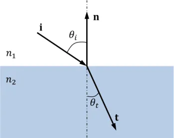
In most underwater imaging systems, a light ray travels through water, housing (glass or plastic) and air. It will be refracted two times on the air-housing and housing-water interfaces. (Treibitz et al., 2012) pointed out that the flat glass slightly shifts the incident ray and this shift is much smaller in magnitude than the angular refraction effect. In this paper, we assume that the glass is infinitely thin, which in particular fits housings for shallow water. The proposed approach focuses on the flat-port perspective camera and assumes that the refraction only happens at the air-water interface and the optical axis of the camera is perpendicular to the refraction interface. The principle of refraction is given by Snell’s law:
sin 𝜃1 sin 𝜃2=𝑛2
𝑛1
(1) where 𝑛1 and 𝑛2 are the indices of refraction (with values of about 1.0 for air and 1.33 for water, depending on composition).
2.1.1 Refractive Back Projection 2D to 3D
De Greve (2006) gives a detailed explanation on how to calculate the direction of a refracted ray, which is derived from Snell’s law. Here the results are given directly:
Figure 1. Refracted ray according to Snell’s law
𝐭 =𝑛1 𝑛2𝐢 + (𝑛1
𝑛2cos 𝜃𝑖− √1 − sin2𝜃𝑡) 𝐧
(2) where 𝐭 denotes the vector of refracted ray, 𝐢 is the vector of incident ray and 𝐧 represents the normal vector of the refraction interface. Herein, according to Snell’s law, sin 𝜃𝑡
can be calculated from sin 𝜃𝑖 and the following formula can be further derived:
sin2𝜃𝑡= (𝑛1
𝑛2)
2
sin2𝜃𝑖= (𝑛1
𝑛2)
2
(1 − cos2𝜃𝑖) (3) Here cos 𝜃𝑖 is the cosine of the supplementary angle between two known vectors 𝐢 and 𝐧, which can be formulated by the dot product of these vectors:
cos 𝜃𝑖= −𝐢 ∙ 𝐧
(4) Above mentioned formulas show that for each ray in 3D space, the refracted ray can be directly calculated from the normal vector of the refraction interface and the refraction indices of the two media.
2.1.2 Refractive Projection 3D to 2D
Estimating the 2D projection of a 3D point through the refraction plane is tricky, because the intersection point on the flat interface is unknown and the ray of the path cannot be defined directly. However, it still follows Fermat’s principle:
The light ray path between two points that takes the least time to transverse.
Figure 2. The ray from a 3D point in the medium intersects the refraction plane, modified from (Treibitz et al., 2012) As it is illustrated in Figure 2, the 3D point embedded in the medium passes through the flat interface and is refracted towards the center of the lens. Due to the symmetry property around the camera optical axis 𝑍 in this model, the 3D coordinate (XP, YP, ZP) can be rewritten to radial representation form (rP, ZP). Then the travelling time of the optical path 𝐿 can be formulated as:
𝐿 = 𝑛2√(r2− r1)2+ 𝑍22+ 𝑛1√r12+ d2
(5) where d denotes the distance from the camera center to the refraction interface. The solution minimizes the travelling time according to its partial derivatives (Glaeser and Schröcker, 2000):
𝜕𝐿
𝜕r1= 𝑛2 r1− r2
√(r2− r1) + Z2+ 𝑛1 r1
√r12+ d2= 0 (6)
𝑛
2𝑛
1𝐢
𝐭 𝐧 𝜃
𝑖𝜃
𝑡lens
𝑛
1𝑍 (
r2, Z2)
𝑛
2(
r1,
d)
d
r
2.2 Attenuation of Light
The loss of radiometric signal through the water body can be attributed to absorption and scattering. Those effects can be formulated in a water-property- and wavelength-dependent model and relate the signal attenuation with distance, proposed by (McGlamery, 1975; Jaffe, 1990). A simplified underwater optical model is expressed below, which is also widely applied in image dehazing:
𝐼(𝑑, 𝜆) = 𝐼0(𝑑) ∙ 𝑒−𝜇(𝜆)𝑑+ 𝐵 ∙ (1 − 𝑒−𝜇(𝜆)𝑑) (7) Here 𝐼 denotes the radiance received by the camera after travelling distance 𝑑 through the water body, 𝐼0 and 𝐵 are the original irradiance from the object and background irradiance of the underwater scene. 𝜇(𝜆) indicates the attenuation coefficient according to different wavelength 𝜆.
3. METHODOLOGY
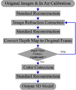
The refinement methodology contains two parts, geometry correction for refraction effects and radiometry correction for attenuation effects. The core of the processing is the refraction correction. The complete reconstruction pipeline by using the proposed new methods can be described as follows:
(1) First, obtain the calibration of the camera in air.
(2) Then import the original underwater images into a standard photogrammetry processing pipeline (in this paper, this part is implemented by the commercial software PhotoScan) to estimate the 3D information with fixed pre-calibration parameters.
(3) Afterwards, use the exported depth maps from last step to correct the refraction effect for each original image.
(4) Convert the depth maps from current corrected image frame to the original image frame.
(5) Iteratively update the refraction corrected images and compute new depth maps until the depth maps between 2 iterations converged.
(6) Once the final geometry refined images are obtained, the color information will be adjusted based on the depth map and the reconstruction result is again updated in order to get the final 3D reconstruction product.
At the first glance it might seem that using the original images in step 1 of the iteration would be inconsistent. Indeed, if there is prior geometry information at the beginning (known ground plane, maximum viewing distance, detected markers, etc.), the images before the first iteration could be undistorted with respect to this geometry. Not undistorting them means that we assume that the entire scene is close to the glass interface of the camera (no refraction). Which of the priors should be used such that the algorithm will converge to the correct 3D scene layout depends on the setting and needs further evaluation. For our first experiments reported in this contribution we start with the
“close scene” assumption.
For practical reasons (holes, noise, artifacts), all the depth maps mentioned in this paper are rendered from the photogrammetric reconstruction – result rather than the raw depth maps from dense matching as they are more complete and consistent.
Another assumption is if there is no depth information in some image area, then the object is assumed to be on a plane which exceeds visibility distance (In this paper, it is set to 15m). To fill small holes, we use a superpixel segmentation of the image and fill missing depth values by interpolating between
neighboring pixels of the same segment. The workflow of the whole processing is illustrated in Figure 3:
Figure 3. Workflow of the proposed iterative refinement 3D reconstruction
3.1 Geometric Refinement Processing
In summary, geometric related processing has two main components: refraction correction and image frame conversion.
Refraction correction corrects the original images in order to eliminate the refraction effect on the image and image frame conversion converts the depth map back to the original image frame which compares the depth value changes for loop decision.
3.1.1 Refraction Correction
Figure 4. Pseudo-code of refraction correction algorithm Refraction correction accesses the known depth value for each pixel, back projects the ray along refracted path to get the 3D point, and then projects the 3D point from the 2D image plane
Input: Color Image with refraction, Depth Map 𝐷, Camera Matrix, distance to refraction plane 𝑑0, refraction indices (air-water)
Output: Refraction corrected Color Image, Refraction corrected Depth Map 𝐷𝑐𝑜𝑟𝑟𝑒𝑐𝑡𝑒𝑑
1 for each pixel (𝑥, 𝑦);
2 Generate the original rays from the camera center to the pixel;
3 Calculate the refracted rays for each original ray by using Equation (2)
4 Back project the 3D point through the refracted ray with the distance of (𝐷(𝑥, 𝑦) −𝑑0)
5 Project the 3D point to image plane (𝑥′, 𝑦′), save as the target coordinates;
6 Create the Delaunay triangulation from the target coordinates with their corresponding depth values and color information.
7 Interpolate the pixel value for the output images;
by using the inverse camera matrix. The target coordinates for each pixel are non-integer values, which demand a scattering interpolation processing to interpolate the pixel values for each pixel in the target image. Pseudo-code in Figure 4 describes the entire procedure for image refraction correction:
3.1.2 Original Image Frame Conversion
The coordinates of the image typically changed after the refraction correction and the current exported depth map cannot be directly compared with the one from the previous iteration.
Also, the correction processing must use the original underwater images, so that the conversion of the new depth map from the refraction corrected image frame to the original image frame is needed. There are two solutions to solve this problem. One solution is applying inverse transformation of the refraction correction. During the refraction correction procedure, the target coordinates for each pixel in the original image have been calculated, which can be stored in a transformation matrix. The transformation matrix records the target pixel coordinates for each pixel, which also can be used for inverse transformation from corrected image frame to original image frame. The image transforming function by using transformation matrix has been implemented in OpenCV cv::remap function (Bradski and Kaehler, 2000).
Another solution is to project the 3D points under the pinhole camera model and to minimize the light travelling time as discussed in Section 2.1.2, to estimate the intersection point on the refraction plane and to derive the supposed pixel coordinate in the refraction scene. Afterwards, apply a procedure similar to the one which described in Figure 4 to interpolate the pixel values for the output images.
3.2 Radiometric Refinement Processing
Once the final depth information for each pixel is obtained, the pixel-wise attenuation correction can be applied according to Equation (7) for each channel. However, due to high attenuation and low signal-to-noise ratio of the red channel, the original irradiance of the red channel cannot be directly recovered from itself. In this paper, an additional white balancing (or more precisely, red channel compensation) is deployed to enhance the red channel information. The corresponding white balancing approach is based on the work from (Ancuti et al., 2011), which compensates the red channel by a linear combination of RGB values of the pixel. In summary, the radiometric refinement processing first corrects the attenuation effect for each pixel in the green and the blue channel, and then compensates the red channel by using RGB channels to form up the new color for each pixel. Since in this paper, the main focus is the geometry correction part, the radiometric refinement processing is only aimed at providing a more appealing color for the 3D model, but does not aim at quantitative correctness.
4. VERIFICATION ON TEST DATASET To verify the proposed geometry refinement approach, an underwater test dataset with ground truth information is required. It should contain refraction effects in the images and good position and geometry information, which is very difficult to obtain in reality. In this paper, a pre-built 3D model was applied as the ground truth data and a set of images were rendered from this model. The air-water refraction effects were added to these images afterwards by applying the refractive ray-tracing on their depth maps. Afterwards, the iterative
refinement approach was evaluated on these test images to verify the improvement in 3D reconstruction.
4.1 Simulation of Underwater Refraction
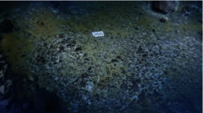
In computer graphics, refraction effects have long been used in order to simulate underwater scenes (Wyman, 2005; Hu and Qin, 2007; Sedlazeck and Koch, 2011). To verity the proposed approach, a 3D model has been generated from underwater footage from a research cruise to the Niua South hydrothermal vent field (Figure 5) (Kwasnitschka et al., 2016a), from which images were synthesized with refraction.
Figure 5. Ground truth model
Figure 6. Pseudo-code of underwater refraction simulation algorithm
First, a standard graphics rendering engine was utilized to render a set of ground truth images without refraction, as well as their depth maps, and then these “as in air” images were converted into refractive underwater images according to the
Input: Ground Truth Image, Depth Map 𝐷, Camera Matrix, distance to refraction plane 𝑑0, refraction indices (air-water) Output: Refracted Color Image
1 Convert Depth Map to a regular triangle net;
2 Get the min & max values from the Depth Map;
3 for each pixel
4 Generate the original rays from the camera center to the pixel;
5 Calculate the refracted rays for each original ray by using Equation (2);
6 Back project the 3D points with min&max depth along the refracted ray and project the points to image plane to form a line;
7 Get all the triangle faces which touch the line in 2D;
8 for each triangle face
9 Check if the refracted ray intersects the triangle face by using Möller-Trumbore intersection algorithm;
10 if (ray hits the face)
11 Select the intersection point with minimum depth;
12 Project the point to the image plane by using the inverse of Camera Matrix;
13 else
14 Back project the point along refracted ray with two times of maximum depth to 3D and project the point to the image plane;
corresponding depth maps. The basic of the refraction simulation algorithm is ray-casting, which finds the first intersection for each ray casted from the observer (camera).
Refractive ray-casting additionally computes the refracted ray from the original casted ray for further intersection calculation.
To implement the ray-casting, the depth map was converted to a 3D triangle mesh net, and then the ray-triangle intersection was calculated by using the Möller-Trumbore intersection algorithm (Möller and Trumbore, 2005). The following Pseudo-code describes the algorithm of the refractive ray-casting approach to convert the in-air image to an underwater (refracted) scene.
4.2 Accuracy Evaluation
The evaluation is performed on the 31 simulated images with refraction effects, from above mentioned 3D model. The in-air calibration result was pre-defined from rendering the images on the graphics engine. The simulated images with refraction were imported into the iterative refinement workflow. After two iterations, the depth map values already converged. Pictures in Figure 7 illustrate the intermediate result after the first iteration.
Figure 7. Rendered ground truth image (top left), rendered refracted image (top right), refraction corrected image (bottom left), converted image from refraction corrected image frame to original input image frame (bottom right). Please note that the bottom right color image is not needed during the workflow, only the converted depth map under the same image frame is used.
Figure 8. Absolute intensity differences between the ground truth images and the refraction corrected images in each iterations (left: first iteration, right: second iteration). For a better visualization, all the values have been amplified with the factor of 10.
Figure 8 demonstrates the difference between the ground truth images and the refraction corrected images. The mean absolute intensity error between two images are 2.5599 and 2.4271 in the range of [0,255], respectively refer to the result from first and second iteration. The statistics of absolute grey value differences also support the hypothesis that the iterative
refinement is bringing the refraction-corrected images closer to the images taken in air without any refraction effects.
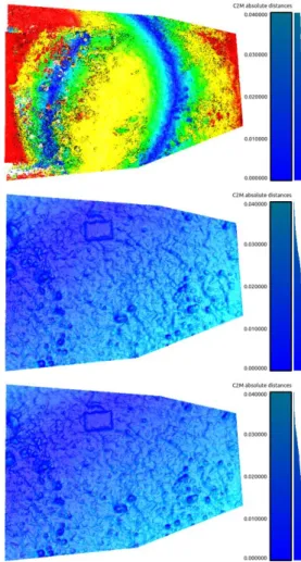
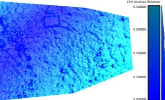
The ground truth model is employed as the reference to evaluate the 3D model quality from different iterations. The area that all models cover is selected and the statistics for the models from each iteration are analysed. As can be seen from Figure 9 and Table 1, after the refraction refinement processing, the absolute distances are improving in the next iteration.
Figure 9. Evaluation of 3D reconstruction from each iteration (The green , yellow, red color in the first picture indicates that the error of this model is much larger than the color bar’s range:
green (0.06m, 0.12m], yellow (0.12m, 0.18m] , red (0.18m, +∞].
Besides the evaluation of the 3D model’s quality in each iteration, an evaluation on the 3D reconstruction under a photogrammetry pipeline with auto calibration mode was also performed. As it is shown in Figure 10, the photogrammetry pipeline with auto calibration mode also provided an appealing model with acceptable accuracy. It estimates the camera intrinsic with a virtual camera and the rest of the refraction effects are compensated by the distortion parameters. However, presumably this is mainly because the selected evaluation area is located in the center of each image, where refraction effects are less severe compared to the pixels on the image boundary.
The proposed approach still has better accuracy in all aspects (see Table 1) than the auto calibration photogrammetry result.
Another advantage of deploying 3D reconstruction by using the proposed approach is that the estimated camera extrinsic can be directly used in other uses (e.g. underwater vehicle navigation) which the auto calibration photogrammetry result cannot
achieve as it is possible that the pose is slightly changed to absorb some of the “un-modelled refraction”-error.
Figure 10. Evaluation of a 3D reconstruction standard photogrammetry pipeline with auto calibration setting
Model Source Evaluation [m]
mean std
Iteration 0 Iteration 1
0.157335 0.014616
0.102416 0.009554 Iteration 2
AutoCalib
0.013680 0.016991
0.008942 0.012032 Table 1. Evaluation statistics of 3D reconstruction in different
steps and methods
5. APPLICATION
During and after the world wars, huge amounts of munitions were dumped into the sea. For instance, an estimated 1.6million tons are still resting on the seafloor of German coastal waters of the Baltic Sea and the North Sea. These munitions not only endanger the environment, people and ships, but they also hinder extension of infrastructure. Besides the risk of explosions, the munitions also contain toxic substances or even chemical agents, which threatening the health of marine ecosystems as well as the food chain and people’s lives. Thus, it is important to locate and map the munitions and to monitor potential drift, deformations and even appearance changes. To monitor the munitions and provide the reference information (especially geometry information) for the government decision, visual 3D reconstruction of the munitions is requested.
One critical site is located in Kolberger Heide, next to Kiel, Schleswig-Holstein, Germany. The test images of munitions (in this case, a torpedo) were taken by a GoPro Hero3 camera within its original underwater flat port housing. The 3D model was generated from 49 images in a very challenging setting for 3D reconstruction, i.e. extremely greenish color in the Baltic Sea, bad visibility and all the images were taken by divers in forward motion.
Figure 11. Original image (left) and refined image (right) The iterative refinement approach was applied on this test dataset, Figure 11 shows one of the original image (left), as well as the refined image (right), after the geometry has been established during the first iteration of pinhole processing. The
color correction was also implemented to demonstrate the improvement on the radiometric aspect. The final 3D model was established from the refined images. Due to the poor visibility, achieving a complete depth map for each image is becoming extremely difficult. Even though the rendered depth map from the 3D model is used to correct the refraction effects for the images, there are still some noticeable discontinuities in the processed images which are so far unresolved. However, the discontinuity region does not cover the body of the torpedo, which didn’t affect the 3D modelling. As it is shown in Figure 12, the refined images represent a useful quality of the 3D model with fine details and the color of the model is also improved.
Figure 12. 3D model of a torpedo in Baltic Sea 6. CONCLUSION AND FURTHER WORK This paper has presented an approach that iteratively removes refraction effects from underwater images for 3D reconstruction, allowing to employ standard photogrammetry packages for refractive image material. The first results on the test and real world dataset indicate that the iterative approach is a promising alternative for generating 3D models from images suffering from flat port refraction and strong attenuation, using traditional pinhole software modules. Still, the iterative nature demands quite some time and several aspects such as depths discontinuities or consequences of the initially assumed geometry before the first iteration and the basin of convergence of the algorithm have to be inspected in more detail in the future.
Also, the iterative refinement concept is only deployed on the geometry correction, whereas (Ancuti et al., 2011) have shown that their radiometric recovering approach is able to enhance the feature matching in the reconstruction pipeline. Integrating the radiometric correction into the iterative processing concept might also here improve the structure from motion and depth estimation.
ACKNOWLEDGEMENTS
This is publication 042 of the DeepSea Monitoring (DSM) Group at GEOMAR. The authors of this paper are grateful for support from the Chinese Scholarship Council (CSC) and the German Federal Ministry for Education and Research in the UDEMM project (03F0747A, B, C). The authors would also like to thank Mareike Kampmeier and the scientific divers for capturing the underwater image materials.
REFERENCES
Agrafiotis, P., Georgopoulos, A., 2015. CAMERA CONSTANT IN THE CASE OF TWO MEDIA PHOTOGRAMMETRY.
ISPRS - International Archives of the Photogrammetry, Remote Sensing and Spatial Information Sciences, XL-5/W5, 1–6.
Agrawal, A., Ramalingam, S., Taguchi, Y. and Chari, V., 2012, June. A theory of multi-layer flat refractive geometry. In 2012 IEEE Conference on Computer Vision and Pattern Recognition (pp. 3346-3353). IEEE.
Ancuti, C.O., Ancuti, C., De Vleeschouwer, C. and Bekaert, P., 2018. Color balance and fusion for underwater image enhancement. IEEE Transactions on Image Processing, 27(1), pp.379-393.
Bradski, G. and Kaehler, A., 2000. OpenCV. Dr. Dobb’s journal of software tools, 3.
De Greve, B., 2006. Reflections and refractions in ray tracing.
URL
http://users.skynet.be/bdegreve/writings/reflection_transmission .pdf (accessed 2019-03-10).
Fryer, J.G. and Fraser, C.S., 1986. On the calibration of underwater cameras. The Photogrammetric Record, 12(67), pp.73-85.
Glaeser, G. and Schröcker, H.P., 2000. Reflections on refractions. Journal for Geometry and Graphics, 4(1), pp.1-18.
Hu, W. and Qin, K., 2007. Interactive approximate rendering of reflections, refractions, and caustics. IEEE Transactions on Visualization and Computer Graphics, 13(1), pp.46-57.
Jaffe, J.S., 1990. Computer modeling and the design of optimal underwater imaging systems. IEEE Journal of Oceanic Engineering, 15(2), pp.101-111.
Jordt, A., 2013. Underwater 3D reconstruction based on physical models for refraction and underwater light propagation (Doctoral dissertation, Christian-Albrechts Universität Kiel).
Jordt, A., Köser, K. and Koch, R., 2016. Refractive 3D reconstruction on underwater images. Methods in Oceanography, 15, pp.90-113.
Kotowski, R., 1988. Phototriangulation in multi-media photogrammetry. International Archives of Photogrammetry and Remote Sensing, 27(B5), pp.324-334.
Kunz, C. and Singh, H., 2008, September. Hemispherical refraction and camera calibration in underwater vision. In OCEANS 2008 (pp. 1-7). IEEE.
Kwasnitschka, T., Köser, K., Duda, A., Jamieson, J.W., Boschen, R., Gartman, A., Hannington, M.D. and Funganitao, C., 2016a, December. Virtual Vents: A Microbathymetrical Survey of the Niua South Hydrothermal Field, NE Lau Basin, Tonga. In AGU Fall Meeting Abstracts.
Kwasnitschka, T., Köser, K., Sticklus, J., Rothenbeck, M., Weiß, T., Wenzlaff, E., Schoening, T., Triebe, L., Steinführer, A., Devey, C. and Greinert, J., 2016b. DeepSurveyCam—A deep ocean optical mapping system. Sensors, 16(2), p.164.
Lavest, J.M., Rives, G. and Lapresté, J.T., 2000, June.
Underwater camera calibration. In European Conference on Computer Vision (pp. 654-668). Springer, Berlin, Heidelberg.
McGlamery, B.L., 1975. Computer analysis and simulation of underwater camera system performance. SIO ref, 75, p.2.
Möller, T. and Trumbore, B., 2005, July. Fast, minimum storage ray/triangle intersection. In ACM SIGGRAPH 2005 Courses (p.
7). ACM.
Sedlazeck, A. and Koch, R., 2011. Simulating deep sea underwater images using physical models for light attenuation, scattering, and refraction.
Skarlatos, D. and Agrafiotis, P., 2018. A Novel Iterative Water Refraction Correction Algorithm for Use in Structure from Motion Photogrammetric Pipeline. Journal of Marine Science and Engineering, 6(3), p.77.
Treibitz, T., Schechner, Y., Kunz, C. and Singh, H., 2012. Flat refractive geometry. IEEE transactions on pattern analysis and machine intelligence, 34(1), pp.51-65.
Wyman, C., 2005, July. An approximate image-space approach for interactive refraction. In ACM transactions on graphics (TOG) (Vol. 24, No. 3, pp. 1050-1053). ACM.