Body size and mobility explain species centralities in the Gulf of California food web

Community ECology 20(2): 149-160, 2019 1585-8553 © The Author(s).

This article is published with Open Access at www.akademiai.com DOI: 10.1556/168.2019.20.2.5

Introduction

Anthropic activities threaten global biodiversity in the oceans by direct causes like overfishing, pollution and habitat destruction (Lotze et al. 2006), or indirectly through eutrophi- cation and climate change (Worm et al. 2000, Harley et al.

2006). Since biodiversity regulates processes (e.g., primary production and nutrient cycling; Worm et al. 2006), prop- erties (e.g., resistance to invasion; Stachowicz et al. 2002) and their maintenance over time and space, its decline has profound consequences on the functioning of ecosystems.

Although causal relationships are difficult to infer, the ac- celerating biodiversity loss is expected to be critical for the provision of goods (e.g., decrease of catch from fisheries;

Worm et al. 2009) and services (e.g., increased exposure to flooding events and loss of nursery habitats; Díaz et al. 2006, Orth et al. 2006) to human populations. This scenario requires effective actions of ecosystem management to arrest the ero- sion and sustain the recovery of biodiversity. The failure of traditional strategies for fisheries management suggested shifting the focus from single species or sectors to actions targeting the whole ecosystem, a principle that lies behind the

approach of “Ecosystem-Based Management” (EBM; Long et al. 2015).

Long et al. (2015) identified fifteen essential elements to successfully implement EBM. Among those elements the consideration of ecosystem connections was classified as of high importance. Such principle can be interpreted as: (1) the connectivity of marine environments, (2) the synergistic ef- fect of multiple stressors and (3) the interactions among spe- cies (Guerry 2005). The first refers to the flow of nutrients and energy that can establish links between marine environ- ments. For example, sub-tidal kelps supply carbon to inter- tidal communities and are vital for maintaining dense popula- tions of patellid limpets in the southwestern rocky shores of South Africa (Bustamante et al. 1995). The second focuses on the fact that the interplay between various perturbations and their impact on ecosystems are often complicated to unveil.

Indeed, in the Black Sea the overexploitation of small pelag- ics started in the 1970s but its consequences were masked ini- tially by the bottom-up effect due to eutrophication (Bodini et al. 2018). The third lies on the assumption that the modelling of trophic interactions can give clues on the spread of indi- rect effects in food webs. Bondavalli and Ulanowicz (1999)

Body size and mobility explain species centralities in the Gulf of California food web

R. Olmo Gilabert

¹

, A. F. Navia

²

, G. De La Cruz-Agüero

¹

, J. C. Molinero

³

, U. Sommer

³

and M. Scotti

^3,4

1CICIMAR Centro Interdisciplinario de Ciencias Marinas del Instituto Politécnico Nacional, Apartado Postal 592, CP 23094, La Paz, Baja California Sur, México

2Fundación colombiana para la investigación y conservación de tiburones y rayas, SQUALUS. Calle 10° # 72-35, Apto. 301E, Cali, Valle, Colombia

3GEOMAR Helmholtz Centre for Ocean Research Kiel, Düsternbrooker Weg 20, 24105 Kiel, Germany

4Corresponding author. Email: marcoscot@gmail.com, phone: +49 (0) 431 600 4405

Keywords: Biodiversity; Centrality indices; Ecosystem functioning; Trait ecology.

Abstract: Anthropic activities impact ecosystems worldwide thus contributing to the rapid erosion of biodiversity. The failure of traditional strategies targeting single species highlighted ecosystems as the most suitable scale to plan biodiversity management.

Network analysis represents an ideal tool to model interactions in ecosystems and centrality indices have been extensively applied to quantify the structural and functional importance of species in food webs. However, many network studies fail in deciphering the ecological mechanisms that lead some species to occupy the most central positions in food webs. To address this question, we built a high-resolution food web of the Gulf of California and quantified species position using 15 centrality indices and the trophic level. We then modelled the values of each index as a function of traits and other attributes (e.g., habitat). We found that body size and mobility are the best predictors of indices that characterize species importance at local, meso- and global scale, especially in presence of data accounting for energy direction. This result extends previous findings that illustrated how a restricted set of trait- axes can predict whether two species interact in food webs. In particular, we show that traits can also help understanding the way species are affected by and mediate indirect effects. The traits allow focusing on the processes that shape the food web, rather than providing case-specific indications as the taxonomy-based approach. We suggest that future network studies should consider the traits to explicitly identify the causal relationships that link anthropic impacts to role changes of species in food webs.

Abbreviations: ESM–Electronic Supplementary Material; EBM–Ecosystem-Based management; SST–Sea Surface Temperature.

150 Olmo Gilabert et al.

showed that intraguild predation can cause unexpected ben- eficial effects of the American alligator upon its prey (e.g., frogs are consumed by both snakes and alligators, but the latter exert stronger predatory impact on snakes than on the common prey). Therefore, to consider ecosystem connections implies emphasis on processes (i.e., interactions) linking ob- jects (e.g., marine environment, sources of stress or species), a perspective shared with the studies of network analysis.

Network analysis represents an ideal tool to model eco- system connections in multitrophic systems, and centrality indices can be calculated to quantify species importance in trophic interaction networks. Scotti and Jordán (2015) found that less abundant species in the Prince William Sound food web are unevenly distributed towards the top of the trophic chain and such network position further accentuates their risk of local extinction, which is already high because of the small population size. Rocchi et al. (2017) proposed network analysis to merge the gap between EBM theory and practice in data-poor contexts. They showed that, in general, the struc- ture of the food web is robust to the removal (i.e., local ex- tinction) of most vulnerable species (i.e., main target of fish- eries) in the coastal ecosystem of Baja California Sur. Studies that rank species using centrality indices assume that being central in the trophic network corresponds to being function- ally important. These studies provide indications based on the taxonomy (i.e., identity of the nodes), without inform- ing about the ecological attributes (e.g., body size, habitat,

spatial and temporal distribution) of the most central species.

The way species traits (and other attributes) are overlooked is in contrast with the goal of understanding how the position of species in the biotic interaction milieu (i.e., the realized niche) is governed by functional traits (McGill et al. 2006).

In this work, a highly disaggregated network of the Gulf of California food web was constructed. Sixteen indices (centralities and trophic level) were computed and regressed against species attributes (i.e., traits, together with features that classify spatial and temporal distribution). The attributes of the species (i.e., nodes) are independent of their network positions and allowed studying the ecological aspects that can explain node centralities and trophic level. Our goals were:

(1) to investigate whether attributes can be used to predict centrality scores of species; and (2) to identify if there exists a restricted set of attributes able to characterize the position of species in the food web.

Methods

Study area

The study area is the Gulf of California, a marginal sea of the Pacific Ocean between the Baja California Peninsula and the Mexican mainland (Fig. 1). It spans from 24º N up to 32º N of latitude and is strongly influenced by the discharge of sediments from the Colorado River, with shallow waters

Altitude (m) 0 550 1100 1650 2200 2750 Legend 32°

31°

30°

29°

28°

27°

26°

25°

24°

23°

-118° -117° -116° -115° -114° -113° -112° -111° -110° -109° -108° -107° -106°

Pacific Ocean

Gulf of Mexico

Caribbean Sea Atlantic Ocean

Figure 1. Map of the Gulf of California where isobaths are visualized and blue colors reflect sea depth. The map was generated with QGIS (version 2.14.20) http://www.qgis.org. The bathymetry was retrieved from the British Oceanographic Data Center (BODC) through the General Bathymetric Chart of the Oceans (GEBCO) https://www.bodc.ac.uk/data/online_delivery/gebco/. The relief layers for the continental area were obtained at a resolution of 60 m from the INEGI website and are based on the Continuo de Elevaciones Mexicano 3.0 (CEM 3.0) - discharge http://www.inegi.org.mx/geo/contenidos/datosrelieve/continental/default.aspx. The map of Mexico in the upper right corner is in vector format; it was obtained from the shape file “Mex_adm1.shp”, which contains the states of the Mexican Republic. The US map layer (grey map on the top right) was obtained from the United States Geological Survey (USGS) https://www.sciencebase.gov/catalog/item/4fb555ebe4b04cb937751db9. All webpages were accessed on November 3, 2018.

Traits and centralities in a marine food web 151

in the north and deeper waters in the southern part (200- 3000 m). The continental shelf is wider on the east coast due to the absence of high flow rivers on the west part. The Gulf of California has a characteristic continental climate, with sea surface temperature (SST) ranging between 13 °C and 31 °C and salinities of 35-35.8 PSU. In the northern part there are four endemic species. Three of them are economically impor- tant for fisheries (Cynoscion othonopterus (Jordan & Gilbert), Micropogonias megalops (Gilbert), and Totoaba macdon- aldi (Gilbert)) while the fourth is Phocoena sinus (Norris &

McFarland), the smallest and most endangered cetacean in the world. The rich biodiversity and the provision of relevant eco- system services (e.g., resources for fisheries) call for the imple- mentation of effective strategies of conservation (Lluch-Cota et al. 2007), an effort highlighted by the presence of 12 protect- ed areas and 5 biosphere reserves (Sánchez-Ibarra et al. 2013).

Food web construction

The food web was constructed using literature data (e.g., gut content analysis; see Electronic Supplementary Material 1, ESM1) and consists of 317 taxa (nodes; n = 317), 74% of which were identified at species level. All nodes stand for living compartments (32 primary producers and 285 con- sumers) and the 3971 trophic interactions (links; l = 3971) are weighted with predator’s feeding preferences, which consider the proportions of food that each predator receives through its prey (i.e., the total amount of food consumed by each predator is set to 1 and the relative contribution of each prey corresponds to the weight of the link). Therefore, the feeding preferences are always included in the interval (0, 1]. The only case with link weight = 1 is when the preda- tor consumes a single prey type (i.e., diet specialization).

Species distribution was validated through maps built with Mapmaker in the ModestR environment (García-Rosello et al. 2013), the Ocean Biogeographic Information System¹ (OBIS) and iSpecies². The diet of 262 nodes (91.93% of the consumers) was defined using literature data specific to taxa that appear in the food web, while surrogate species (i.e., species that belong to the same genus, with compara- ble body size and maximum depth distribution) were con- sidered for the remaining 23 nodes (8.07%; ESM1 at page 15). In particular, the diet of 186 consumers (65.26%) is based on information from the Gulf of California or areas nearby (i.e., Pacific Ocean in front of California and Central America). Main objectives were constructing a high resolu- tion food web with most nodes representing single species and retrieving information on feeding preferences. All flows of energy from prey/resources (first column) to predators/

consumers (second column), together with feeding prefer- ences (third column), are stored in the ESM2 (text file with tab-separated values).

1 www.iobis.org 2 www.ispecies.org

[both websites last accessed on November 3, 2018]

Attributes of the taxa

To investigate the ecological meaning of various cen- trality indices we built a database including different at- tributes (e.g., traits and habitat; see ESM1). Metadata con- cerning all nodes were collected and the centrality scores (dependent variables) were regressed against the ecological attributes (independent variables). The following attributes were taken into account: (1) body size (classes of maximum body length measured in cm, with intervals representing 10- fold increases), (2) habitat (nine categories: reef, benthic, benthic-neritic, benthic-pelagic, pelagic-neritic, demersal- neritic, pelagic, pelagic-oceanic, or demersal), (3) maxi- mum depth (to distinguish among: species close to surface (0,10] m, subtidal zone close to coast and reefs (10, 100]

m, continental shelf (100, 200] m, continental slope in the upper part of mesopelagic zone (200, 500] m, lower part of mesopelagic zone (500, 1000] m, aphotic zone (1000, 2000] m, or deeper zones where large size migrants can live (2000, 3000] m), (4) mobility (i.e., taxa were classified as sessile or moving at various velocities: “low” for taxa dis- playing mainly passive movements that cannot be efficient for predator avoidance; “medium” that indicates the capa- bility to move actively to escape from predators, referring to movements restricted to specific systems as seagrass beds and coral reefs; “high” that is used for species that move fast and cross different habitats), (5) direction of spatial move- ment (absence of move, move in latitude and/or longitude, water column move, movements both in latitude/longitude and water column), (6) seasonality (present in summer, win- ter, or both seasons), (7) daily activity (diurnal, nocturnal, or both), and (8) congregatory behavior (e.g., schooling for fish; it includes two classes: yes or no). Altogether, 2536 traits were considered and 89.04% of them was retrieved from the literature for taxa present in the food web. The re- maining 10.96% was estimated with the opinion of experts (Prof. Gustavo De La Cruz-Agüero and Dr. Andrés Felipe Navia). The traits not found in the literature refer to: body size (20 nodes), daily activity (147 nodes) and congregatory behavior (111 nodes). The attributes of each node are in the ESM3. Frequency distributions of the eight attributes are reported in the ESM1, Fig. S1.

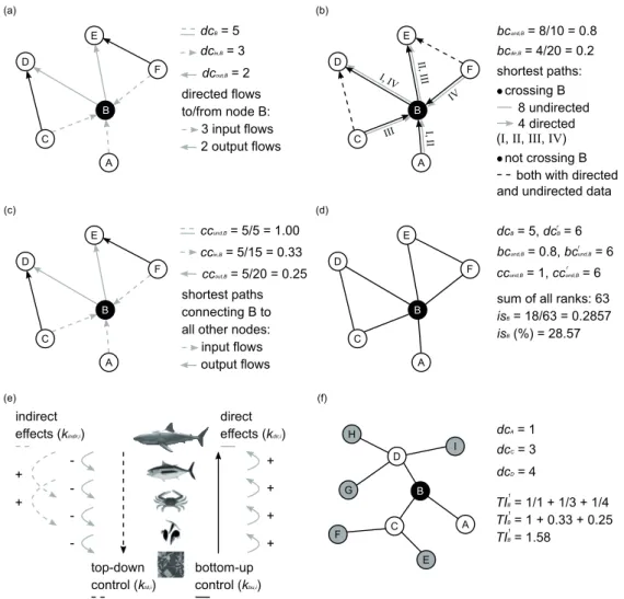
Centrality indices and trophic level

Centrality indices were selected to model the importance of nodes with respect to energy circulation and the spread of indirect effects in the food web. The position of each node i in was characterized by degree, betweenness, closeness, im- portance score, keystone indices and topological importance (Fig. 2). Such indices were chosen for their capability of de- scribing node importance from local to global network scale, taking into account the diffusion of both vertical (i.e., bottom- up and top-down) and horizontal (e.g., to discriminate among trophic cascade and apparent competition) effects (Scotti and Jordán 2015). Feeding preferences were used to calculate the weighted forms of betweenness and closeness centralities.

All other indices were presented in the unweighted version as

152 Olmo Gilabert et al.

they were computed using the architecture of trophic interac- tions only. The centrality indices account for the role of the nodes at local (degree), meso- (keystone indices and topolog- ical importance), and global scale (closeness, betweenness, and importance score). In addition to the centrality indices also the trophic level was quantifi ed. The trophic level of each consumer depends on the set of resources eaten; the contri- bution of the resources is then weighted by considering the feeding preferences of the consumer.

The degree of i is the sum of all directed interactions in which the node is involved (dc_i); it can be decomposed into in-degree (total number of prey/resources; dc_in,i) and out-de- gree (total number of predators/consumers; dc_out,i) (Jordán et al. 2006):

dci = dcin,i + dcout,i (1)

Betweenness centrality measures how frequently a node i lies on the shortest paths (i.e., geodesics) connecting any pair of nodes j and k in the network (Jordán et al. 2006).

Betweenness can be calculated either by considering the di-

rectionality of fl ows (directed betweenness; bc_dir,i) or ignoring it (undirected betweenness; bc_und,i); the fi rst accounts for the importance of nodes in spreading bottom-up effects, while the second combines vertical (bottom-up and top-down) and horizontal effects. In presence of undirected data, and in a network of n nodes, the normalized betweenness is:

(2) where cjk is the total number of shortest paths between j and k, and cjk(i) are the geodesics linking j with k and crossing i.

The total score is computed by summing the relative number of times the geodesics between all pairs of nodes pass through i. The denominator is used to normalize the total score and stands for the number of all pairs of nodes excluding i.

Directed betweenness is calculated in analogy with (2), and the only modifi cation concerns the normalization that uses [(n–1)(n–2)] as denominator. Nodes with high betweenness

(b) (a)

dc^B = 5 dc^in,B = 3

dc^out,B = 2 directed flows to/from node B:

2 output flows 3 input flows A

C D

E

F B

A B C

D

E

F

I, II I, IV

II, I II

IV III

bc^und,B = 8/10 = 0.8

shortest paths:

bc^dir,B = 4/20 = 0.2

and undirected databoth with directed - not crossing B

4 directed 8 undirected (I, II, III, IV) - crossing B

(e) (f)

dc^A = 1 dc^C = 3 dc^D = 4 TI^B TI^B

TI = 1/1 + 1/3 + 1/4 TI^B

TI^B

TI^BB = 1 + 0.33 + 0.25 = 1 + 0.33 + 0.25

1

TI^B TI^B TI^BB1 = 1.58 = 1.58

1

C D

A B

E F

H

G

I

top-down

control (kkk^td,itd,i) bottom-up control (kkk^bu,ibu,i)

direct effects (kkk^dir,idir,i) indirect

effects (kkk^{indir,iindir,i}) - + +

+ -

- -

+ + +

(d)

A B C

D

E

F

sum of all ranks: 63 is^B = 18/63 = 0.2857 is^BBB (%) = 28.57 (%) = 28.57 dc^B = 5, dc^Br = 6 bc^und,B = 0.8, bc^und,Br = 6 cc^und,B = 1, cc^und,Br = 6 (c)

shortest paths connecting B to all other nodes:

output flows input flows

cc^und,B = 5/5 = 1.00

cc^out,B = 5/20 = 0.25

cc^in,B = 5/15 = 0.33

A C

D

E

F B

Figure 2. Schematic representation of centrality indices used in this study. These indices quantify the role of nodes with reference to lo- cal (degree, a), global (betweenness, b; closeness, c; and importance score, d), and meso- (all keystone indices but k_dir,i, which accounts for local effects only - see Fig. 3, e; and topological importance, f) scales. In the fi rst three charts (a-c) the arrow-headed links leave the prey and point to predators. Conceptual diagram is illustrated for the keystone indices while all other centralities are calculated for node B.

Page 152, Equation (2) – replace the first comma with semicolon: “…; i ≠ j ≠ k,…” – see below 𝑏𝑏𝑏𝑏_{𝑢𝑢𝑢𝑢𝑢𝑢,𝑖𝑖}=^{∑ ∑}

𝐶𝐶𝑗𝑗𝑗𝑗(𝑖𝑖) 𝐶𝐶𝑗𝑗𝑗𝑗 𝑛𝑛𝑗𝑗=1 𝑛𝑛𝑗𝑗=1

(𝑛𝑛−1)(𝑛𝑛−2) 2

; 𝑖𝑖 ≠ 𝑗𝑗 ≠ 𝑘𝑘 (2)

Page 153, Equation (3) – the sum goes from “k=1” and not “j=1” as currently indicated:

𝑏𝑏𝑏𝑏_{𝑖𝑖𝑢𝑢,𝑖𝑖}= [^{∑𝑛𝑛𝑗𝑗=1}_𝑢𝑢−1^{𝑢𝑢(𝑝𝑝𝑗𝑗,𝑝𝑝𝑖𝑖)}]⁻¹ (3)

Page 153, Equation (8) – the last term should be “ktd,i” and not “ktd,z”:

𝑘𝑘_𝑖𝑖= 𝑘𝑘_{𝑏𝑏𝑢𝑢,𝑖𝑖}+ 𝑘𝑘_{𝑡𝑡𝑢𝑢,𝑖𝑖} (8)

Page 154, Equation (17) should be written as follows:

𝑇𝑇𝑇𝑇_𝑖𝑖^𝑚𝑚=^{∑𝑚𝑚𝑧𝑧=1}_𝑚𝑚^{𝛽𝛽𝑧𝑧,𝑖𝑖}=^{∑𝑚𝑚𝑧𝑧=1∑}_𝑚𝑚^{𝑛𝑛𝑗𝑗=1𝑎𝑎𝑧𝑧,𝑗𝑗𝑖𝑖} (17)

Traits and centralities in a marine food web 153

are in the shortest paths linking many pairs of nodes and are expected to play relevant role in the spread of indirect effects.

Closeness centrality depends on the length of geodesics connecting a given node i to all other nodes in the network (Jordán et al. 2006). Undirected closeness is computed using the shortest paths linking node i to all other nodes, irrespec- tive of energy flow direction (cc_und,i). Two directed versions can be calculated when shortest paths detection is constrained by energy flow orientation (i.e., strict bottom-up perspective):

(a) in-closeness (cc_in,i) accounts for shortest paths from all network nodes to a given node i, while (b) out-closeness (cc_out,i) is based on the shortest paths from a given node i to all other network nodes. In directed networks there might be nodes that are not reachable when following the energy flow (e.g., two nodes that are apical predators); in such cases the shortest path is conventionally set as equal to n. In-closeness is obtained by summing all shortest paths to node i, and the size of the network (n) is used to normalize the score (the denominator is the number of all nodes except the one for which closeness is computed):

(3)

where d(p_k,p_i) is the number of steps in the geodesics linking the nodes k to i. Out-closeness is calculated according to the same principle, but considering all shortest paths from node i:

d(p_i,p_k). The equation for cc_und,i has the same form of (3) but the search of geodesics from and to i does not depend on ener- gy flow orientation. Thus, undirected closeness indicates how fast perturbations of specific nodes can propagate through the food web, irrespective of energy flow direction. Undirected closeness can also give clues on the exposure of each node to perturbations that target any other node in the food web, with the spread of effects not constrained by energy flow direction.

In the directed versions of closeness, the shortest paths follow the direction of energy circulation and spread perturbations either from low trophic level nodes to the target taxa (when the in-closeness of this latter is calculated) or from the target taxa to higher trophic level nodes (when the out-closeness of the target node is computed). Therefore, in-closeness quanti- fies how fast a given node can be affected by perturbations on other nodes, while out-closeness defines how fast the pertur- bation targeting a specific node can diffuse to the rest of the network. Large values are found for: (a) nodes that can be quickly influenced by perturbations of various food web spe- cies (cc_und,i and cc_in,i), and (b) nodes the disturbance of which can rapidly spread and affect many species in the food web (cc_und,i and cc_out,i).

The focus of degree centrality is on local interactions, while betweenness and closeness characterize node position under a whole-network perspective (by taking into account the relative position compared to all pairs of nodes or all other nodes, respectively). In the attempt of simultaneously consid- ering these alternative aspects, an importance score (is_i) was calculated for each node i by combining the local and global information portrayed by degree, undirected betweenness and

undirected closeness. These indices were selected because they are the most widely used centralities in food web analy- sis (e.g., see Scotti and Jordán 2010, 2015). First, for each centrality the nodes were ranked in descending order (i.e., the value of the most central node is 317). Second, for each node i the rank values (denoted by the r superscripts) were summed:

(4) Finally, each score in (4) was normalized by dividing it with the sum of all cumulative ranks:

(5) The meso-scale importance of any given node i was char- acterized by the keystone index (ki) (Jordán et al. 2006). Such index requires as input the binary matrix of trophic interac- tions without cycles. It is calculated by summing bottom-up (kbu,i) and top-down (ktd,i) keystone indices

(6)

(7)

(8) where m is the number of predators feeding on species i and q is the number of prey eaten by species i; dc_in,j is the number of prey of j (in-degree) and dcout,z is the number of predators of z (out-degree). The term k_bu,j stands for the bottom-up keystone index of predator j, while k_td,z indicates the top-down key- stone index of prey z. Both the bottom-up and the top-down variants include parts that refer to direct and indirect effects.

Therefore, the keystone index can be rewritten by summing two other terms: the keystone indices of direct (kdir,i) and in- direct (k_indir,i) effects

(9)

(10) (11) Both k_bu,i + k_td,i and k_dir,i + k_indir,i equal k_i. The keystone index k_i is particularly suitable to quantify the relevance of vertical interactions over horizontal ones, being thus appro- priate for identifying the impacts related to trophic cascade rather than those due to apparent competition.

Topological importance was used to model meso-scale effects by also taking into account exploitative and appar- ent competitions (Jordán et al. 2006). This index considers Page 152, Equation (2) – replace the first comma with semicolon: “…; i ≠ j ≠ k,…” – see below

𝑏𝑏𝑏𝑏_{𝑢𝑢𝑢𝑢𝑢𝑢,𝑖𝑖}=^{∑ ∑}

𝐶𝐶𝑗𝑗𝑗𝑗(𝑖𝑖) 𝐶𝐶𝑗𝑗𝑗𝑗 𝑛𝑛𝑗𝑗=1 𝑛𝑛𝑗𝑗=1

(𝑛𝑛−1)(𝑛𝑛−2) 2

; 𝑖𝑖 ≠ 𝑗𝑗 ≠ 𝑘𝑘 (2)

Page 153, Equation (3) – the sum goes from “k=1” and not “j=1” as currently indicated:

𝑏𝑏𝑏𝑏_{𝑖𝑖𝑢𝑢,𝑖𝑖}= [^{∑𝑛𝑛𝑗𝑗=1}_𝑢𝑢−1^{𝑢𝑢(𝑝𝑝𝑗𝑗,𝑝𝑝𝑖𝑖)}]⁻¹ (3)

Page 153, Equation (8) – the last term should be “ktd,i” and not “ktd,z”:

𝑘𝑘_𝑖𝑖= 𝑘𝑘_{𝑏𝑏𝑢𝑢,𝑖𝑖}+ 𝑘𝑘_{𝑡𝑡𝑢𝑢,𝑖𝑖} (8)

Page 154, Equation (17) should be written as follows:

𝑇𝑇𝑇𝑇_𝑖𝑖^𝑚𝑚=^{∑𝑚𝑚𝑧𝑧=1}_𝑚𝑚^{𝛽𝛽𝑧𝑧,𝑖𝑖}=^{∑𝑚𝑚𝑧𝑧=1∑}_𝑚𝑚^{𝑛𝑛𝑗𝑗=1𝑎𝑎𝑧𝑧,𝑗𝑗𝑖𝑖} (17)

1

bcund,i

=

i, j k

/ ) n )(

n (

c ) i ( c

n j

n

k jk

jk



 



  

2 2 1

1 1

,

1 2

ccin,i

=

1 1

1























 n

) p , p (

nd

j k i

3

4

r i, r und

i, r und

i bc cc

dc  

5 6

isi

=

  





 n j

r ,j r und

j , r und j

r i, r und

i, r und i

cc bc dc

cc bc dc

1

7

kbu,i

=

 

 m

j bu,j

j , in

dc k

1 1 (1 )

8

ktd,i

=

 

 q

z tdz,

z, out

dc k

1 1 (1 )

9

ki

=

kbui,ktd,z

10 11

kdir,i

=

 

 

m j

q z out,z j

,

in dc

dc

1 1

1

12

1

kindir,i

=

 

 

m j

q z out,z

z , td j , in

j, bu

dc k dc

k

1 1

13

ki

=

kdiri,kindiri,

14

 

 

m j

q z out,z j

,

in dc

dc

1 1

1

15

1

m,i

=



 n j am,ij

16

1

m TI m

m z z,ji m

z zi, im

 

 ^{1 1}

17

 



  n

j j ji

i TL g

TL 1 1

18

1

bcund,i

=

i, j k

/ ) n )(

n (

c ) i ( c

n j

n

k jk

jk



 



  

2 2 1

1 1

,

1

2

cc_in,i

=

1 1

1























 n

) p , p (

nd

j k i

3

4

r i, r und

i, r und

i bc cc

dc  

5 6

isi

=

  





 n j

r ,j r und

j , r und j

r i, r und

i, r und i

cc bc dc

cc bc dc

1

7

k_bu,i

=

^{ }

 m

j bu,j

j , in

dc k

1 1 (1 )

8

k_td,i

=

 

 q

z tdz,

z,

out k

dc

1 1 (1 )

9

ki

=

kbui,ktd,z

10 11

kdir,i

=

^{ }

 

m j

q z out,z j

,

in dc

dc

1 1

1

12

1

k_indir,i

=

 

 

m j

q z out,z

z , td j , in

j, bu

dc k dc k

1 1

13

k_i

=

kdiri,kindiri,

14

 

 

m j

q z out,z j

,

in dc

dc

1 1

1

15

1

m,i

=



 n j am,ij

16

1

m TI m

m z z,ji m

z zi, im



^{1 1}

17

 



  n

j j ji

i TL g

TL 1 1

18

1

bc_und,i

=

i, j k

/ ) n )(

n (

c ) i ( c

n j

n

k jk

jk



 



  

2 2 1

1 1

,

1

2

cc_in,i

=

1 1

1























 n

) p , p (

nd

j k i

3

4

r i, r und

i, r und

i bc cc

dc  

5 6

isi

=

  





 n j

r ,j r und

j , r und j

r i, r und

i, r und i

cc bc dc

cc bc dc

1

7

kbu,i

=

 

 m

j bu,j

j , in

dc k

1 1 (1 )

8

ktd,i

=

 

 q

z tdz,

z, out

dc k

1 1 (1 )

9

ki

=

kbui,ktd,z

10 11

kdir,i

=

 

 

m j

q z out,z j

,

in dc

dc

1 1

1

12

1

kindir,i

=

 

 

m j

q z out,z

z , td j , in

j, bu

dc k dc

k

1 1

13

ki

=

kdiri,kindiri,

14

 

 

m j

q z out,z j

,

in dc

dc

1 1

1

15

1

m,i

=



 n j am,ij

16

1

m TI m

m z z,ji m

z zi, im



^{1 1}

17

 



  n

j j ji

i TL g

TL 1 1

18

1

bcund,i

=

i, j k

/ ) n )(

n (

c ) i ( c

n j

n

k jk

jk



 



  

2 2 1

1 1

,

1

2

cc_in,i

=

1 1

1























 n

) p , p (

nd

j k i

3

4

r i, r und

i, r und

i bc cc

dc  

5 6

isi

=

  





 n j

r ,j r und

j , r und j

r i, r und

i, r und i

cc bc dc

cc bc dc

1

7

kbu,i

=

 

 m

j bu,j

j , in

dc k

1 1 (1 )

8

k_td,i

=

^{ }

 q

z tdz,

z, out

dc k

1 1 (1 )

9

ki

=

kbui,ktd,z

10 11

kdir,i

=

 

 

m j

q z out,z j

,

in dc

dc

1 1

1

12

1

k_indir,i

=

 

 

m j

q z out,z

z , td j , in

j, bu

dc k dc

k

1 1

13

ki

=

k_diri,k_indiri,

14

 

 

m j

q z out,z j

,

in dc

dc

1 1

1

15

1

_m,i

=



 n j am,ij

16

1

m TI m

m z z,ji m

z zi, im



^{1 1}

17

 



  n

j j ji

i TL g

TL 1 1

18

Page 152, Equation (2) – replace the first comma with semicolon: “…; i ≠ j ≠ k,…” – see below 𝑏𝑏𝑏𝑏_{𝑢𝑢𝑢𝑢𝑢𝑢,𝑖𝑖}=^{∑ ∑}

𝐶𝐶𝑗𝑗𝑗𝑗(𝑖𝑖) 𝐶𝐶𝑗𝑗𝑗𝑗 𝑛𝑛𝑗𝑗=1 𝑛𝑛𝑗𝑗=1

(𝑛𝑛−1)(𝑛𝑛−2) 2

; 𝑖𝑖 ≠ 𝑗𝑗 ≠ 𝑘𝑘 (2)

Page 153, Equation (3) – the sum goes from “k=1” and not “j=1” as currently indicated:

𝑏𝑏𝑏𝑏_{𝑖𝑖𝑢𝑢,𝑖𝑖}= [^{∑𝑛𝑛𝑗𝑗=1}_𝑢𝑢−1^{𝑢𝑢(𝑝𝑝𝑗𝑗,𝑝𝑝𝑖𝑖)}]⁻¹ (3)

Page 153, Equation (8) – the last term should be “ktd,i” and not “ktd,z”:

𝑘𝑘_𝑖𝑖= 𝑘𝑘_{𝑏𝑏𝑢𝑢,𝑖𝑖}+ 𝑘𝑘_{𝑡𝑡𝑢𝑢,𝑖𝑖} (8)

Page 154, Equation (17) should be written as follows:

𝑇𝑇𝑇𝑇_𝑖𝑖^𝑚𝑚=^{∑𝑚𝑚𝑧𝑧=1}_𝑚𝑚^{𝛽𝛽𝑧𝑧,𝑖𝑖}=^{∑𝑚𝑚𝑧𝑧=1∑}_𝑚𝑚^{𝑛𝑛𝑗𝑗=1𝑎𝑎𝑧𝑧,𝑗𝑗𝑖𝑖} (17)