p a p e r
WINDOWS: Finite Aperture Effects and Applications in Signal Processing
fred harris,
San Diego State University
1. INTRODUCTION:
A
window is the aperture through we exam- ine the world. By necessity, any time or spatial signal we observe, collect, and process must have bounded support. Similarly, any time or spatial signal we approximate, design, and synthesize must also have bounded support.Support is the range or width of the independent variable (time, distance, or frequency) over which the dependent variable, say the signal, is non- zero. This finite support can be defined over mul- tiple dimensions, extending for instance, over a line, a plane, or a volume. Windows can be con- tinuous functions or discrete sequences defined over their appropriate finite supports.
At the simplest level, a window can be considered a multiplicative operator that turns on the signal within the finite support and turns it off outside that same support. This operator effects the sig- nal's Fourier Transform in a number of undesired ways; the most significant of which is undesired out-of-band side-lobe levels. The size and order of the discontinuities exhibited by the signal governs the level and rate of attenuation of these spectral side-lobes. Other unwanted effects include spec- tral smearing and in-band ripple. The design and
or controlling the undesired artifacts of in-band ripple, out-of-band side-lobes, and spectral smearing.
Examples of the application of windows to con- trol finite aperture effects can be found hi numer- ous disciplines. These include the following:
i. Finite duration Impulse Response (FIR) Filter Design:
Windows applied to a prototype filter's Impulse Response to control transition bandwidth, in-band and out-of-band side- lobe levels,
ii. Spectrum Analysis, Transforms of Sliding, Overlapped, Windowed Data:
Windows applied to observed time series to control Variance of Spectral Estimate while suppressing Spectral Leakage (addi tive bias).
iii. Power Spectra as Transform of Windowed Correlation Functions:
Windows applied to sample correlation function to suppress segments of the sam ple correlation function exhibiting high bias and variance.
iv.Non Stationary Spectra and Model Estimates:
Windows applied to delayed and over
and spectral features (model parameters) of non-stationary signals.
v.Modulation Spectral Mask Control:
Design of modulation envelope to control spectral side-lobe behavior.
vi.Synthetic Aperture RADAR (SAR):
Windows applied to spatial series to con- trol Antenna Side-lobes
vii.Phased Array Antenna Shading Function:
Window applied to spatial function to con trol Antenna Side-lobes
viii.Photolithography Apodizing Function:
Smooth Transmission Function applied to optical aperture to control diffraction pat tern side - lobes
We will discuss a subset of these applications later in this chapter. For convenience and consistency, we will consider the window as being applied to a time domain signal. The window can, of course, be applied to any function with the same intent and goal. The common theme of these applica- tions is control of envelope smoothness in the time domain to obtain desired properties in the frequency domain.
2. WINDOWS IN SPECTRUM ANALYSIS:
A concept we now take for granted is that a signal can be described in different coordinate systems and that there is engineering value in examining a signal described in an alternate basis system.
One basis system we find particularly useful is the set of complex exponentials, The attraction of this basis set is that complex exponentials are the eigen-functions and eigen-series of linear time invariant (LTI) differential and difference opera- tors respectively. Put in its simplest form, this means that when a sinewave is applied to an LTI filter the steady state system response is a scaled version of the same sinewave. The system can only affect the complex amplitude (magnitude and phase) of the sinewave but can never change its frequency. Consequently complex sinusoids
have become a standard tool to probe and describe LTI systems. The process of describing a signal as a summation of scaled sinusoids is stan- dard Fourier transform analysis. The Fourier Transform and Fourier Series, shown on the left and right hand side of (1), permits us to describe signals equally well in both the time domain and the frequency domain.
Since the complex exponentials have infinite sup- port, the limits of integration in the forward trans- form (time- to- frequency) are from minus to plus infinity. As observed earlier, all signals of engi- neering interest have finite support, which moti- vates us to modify the limits of integration of the Fourier transform to reflect this restriction. This is shown in (2) where Tsup and N define the finite supports of the signal.
The two versions of the transform can be merged in a single compact form if we use a finite support window to limit the signal to the appropriate finite support interval, as opposed to using the
dt e t h H +∞
∫
j t∞
−
= − ω
ω) ( ) (
ω π H ω e ωd ht +∞
∫
j t∞
−
= ( ) +
2 1
∑
+∞∞
−
= h n e−j t
H(θ) ( ) θ θ π θ
π ο
θ d e H n
h +
∫
jn−
= ( ) +
2 ) 1 (
(1)
dt e t h H
T
t j
SUP =
∫
−sup
) ( )
(ω ω
ω π ω
ωd e H
t
h SUP +j t
+∞
∞
−
∫
= ( )
2 ) 1 (
∑
−=
N
n j
SUP h n e
H (θ) ( ) θ θ θ θ
π π
d e H
n
h SUP −jn
+
−
∫
= ( )
)
( (2)
limits of integration or limits of summation. This is shown in (3).
A natural question to ask when examining (3) is how has limiting the signal extent with the multi- plicative window affected the transform of the signal? The simple answer is related to the rela- tionship that multiplication of two functions (or sequences) in the time (or sequence) domain is equivalent to convolution of their spectra in the frequency domain. As shown in (4), the transform of the windowed signal is the convolution of the transform of the signal with the transform of the window.
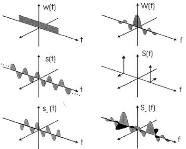
This relationship and its impact on spectral analy- sis can be dramatically illustrated by examining the Fourier transform of a single sinusoid on an infinite support and on a finite support. Figure 1
shows the time and frequency representation of the rectangle window, of a sinusoid of infinite duration, and of a finite support sinusoid obtained as a product of the previous two signals.
Equations (5a) and (5b) describe the same signals and their corresponding transforms.
As we can see, the transform of THe windowed sinusoid, being the convolution of a pair of spec- dt
e t h t w H
HSUP W +∞
∫
j t∞
−
⋅ −
=
= ω ω
ω) ( ) ( ) ( ) (
ω π H ω e ωd t
h W +j t
+∞
∞
−
∫
= ( )
2 ) 1 (
∑
+∞∞
−
⋅ −
=
= W jn
SUP H w n h n e
H (θ) (θ) ( ) ( ) θ θ
π θ θ
π π
d e H n
h W −jn
+
−
∫
= ( )
2 ) 1
( (3)
+∞
∫
∞
−
−
⋅
= λ λ λ
ω π H W d
Hw ( ) ( )
2 ) 1 (
+
∫
−
−
⋅
= π
π
λ λ θ π λ
θ H W d
Hw ( ) ( )
2 ) 1 (
π ω
ω h t e ωd H( )=21 −+∞
∫
∞ ( ) −j tπ ω
ω w t e ωd W
T
T
t
∫
j +−
= −
2 /
2 /
) 2 (
) 1 (
∑
+∞−∞ −= h n e jn H(θ) ( ) θ
+
∑
−
= /2 − 2 /
) ( )
( N
N
n
e j
n w
W θ θ
(4)
: :
0: 2 2
) 1 (
− < <
= Otherwise t T T t
w
fT T fT f
W π
π ) ) sin(
( =
+∞
<
<
∞
−
= t
t f A
t
s( ) sin(2π 0 φ):
) 2 (
) 2 (
) |
( 0 Ae f f0
f f Ae
f
S = −jϕδ − + +jϕδ +
: ) 2
sin(
)
(t =A πf0t−φ sw
) ) (
(
) ) (
sin(
2
) (
(
) ) (
sin(
) 2 (
0 0
) 0
0
T f f
T f e f
AT
T f f
T f e f
f AT S
j
j w
+ + +
−
= −
+
−
π π
π π
ϕ ϕ
2 2
t T T < <+
− (5a)
: :
0: 2 2
) 1 (
− < <
= Otherwise n N N n
w
2) sin( 1
2) sin(
) (
θ θ θ
N T
W =
+∞
<
<
∞
−
= t
n A
n
s( ) sin(θ0 φ):
) 2 (
) 2 (
) |
(θ = −jϕδ θ −θ0 + Ae+jϕδ θ +θ0 Ae
S
: ) sin(
)
(n =A θ0n−φ sw
) 2 sin((
) 2 sin((
) 2 2 sin(( 1
2) ) sin((
) 2 (
0 0
) 0 0
N N Ae
N Ae
Sw j j
θ θ
θ θ θ
θ θ
θ ϕ θ ϕ
+ + +
−
= − − +
2 2
n N N < <+
− (5b)
tral impulses located at f= ±f0 with sin(πfT)/(πfT) or sinc(πfT), the transform of the window, results in the window's transform being scaled and trans- lated to the frequency of the impulses. This can be considered as a special case of the modulation theorem shown in (6) where we can consider me time function h(t) to be the window w(t).
MODULATION THEOREM :
if h(t) has a transform H(f), then h(t) ej2πf0t has a transform H(f - fo)
The effects of the window on the spectrum of a signal can be readily seen in Fig 1. Here we note that the Fourier transform of the constant enve- lope sinusoid has zero width. The first effect we observe is a smearing of me transform's spectral width (from infinitesimally small to the main lobe of the sin(πT)/(πfT)). The second effect is spectral leakage, the spreading of the singularity to the sin(πfT)/(πf) side-lobes, a function occupying an infinite support with an envelope exhibiting a spectral decay rate of 1/f.
The side-lobe structure of the windowed trans-
form limits the ability of the transform todetect spectral components of significantly lower ampli- tude in the presence of a large amplitude compo- nent while the main-lobe width of the windowed transform limits the ability of the transform to resolve or separate nearby spectral components.
The first of these limitations is demonstrated in figure 2 where a stylized power spectrum of two sinusoids of infinite extent and of finite extent is presented. For this example, the relative ampli- tude of the low-level signal at frequency f2is 60 dB below the high level signal at f1. Note that the side-lobe structure of the high level signal is greater than the main lobe level of the low-level signal, hence masks the presence of the low-level signal. If the low-level signal is to be detected in the presence of the nearby high level signal, the window applied to the data must be modified.
Windows must be selected with side-lobe struc- ture significantly lower than the side-lobe struc- ture of the rectangle window.
A comment is called for here on this example.
Under the restricted condition that the frequen-
(6)
Figure 1. Time and Spectral Description of Rectangle Window, Sinusiod and Windowed Sinusoid
Figure 2. Spectral Representation of Un-windowed and of a Rectangle Windowed Sinusoids of Significantly Different Amplitudes
cies of the two signals are harmonically related to the observation interval, (that is that the two sig- nals each exhibit an integer number of cycles in the observation interval), the two signals would be resolvable and measurable. This is because, for the conditions described, the two signals are orthogonal, which when interpreted in the fre- quency domain means that the spectrum of the second signal is located on a zero crossing of the spectrum of the first signal. We will discuss this special condition and similar examples in the sec- tion on windows and the discrete Fourier trans- form (DFT).
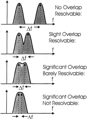
As mentioned earlier, the main-lobe width of the windowed transform limits the ability of the transform to resolve closely spaced spectral com- ponents of comparable amplitudes. This limita- tion is demonstrated in figure 3. where we demonstrate loss of resolvability of two signals as the spectra of two sinusoids of finite support are brought closer together.
For this example, the amplitude of the two sig- nals is the same and the interaction between the phase of the main-lobes and the interaction between the main-lobes and the neighbor's side- lobes has been ignored. It is apparent that the spacing between adjacent spectral lines that can be resolved by a windowed transform is related to the main-lobe width of the window's spectrum.
For the rectangle window, this main-lobe width (measured from peak to first zero crossing) is 1/T, the reciprocal of the window's duration in the time domain. We will find in the next section, that as we modify windows to obtain a desired reduc- tion in side-lobe levels, this side-lobe reduction is accompanied by an increase in main-lobe width which reduces the spectral resolution capabilities of the window.
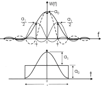
3. WINDOWS AS A SUM OF COSINES We can not build windows without side-lobes in their spectra. What we can do is design windows with arbitrarily low level side-lobes. We can accomplish this with a number of
design tools, which we will examine shortly. The common mechanism of these tools is that they control side-lobe levels by controlling the smooth- ness of the window in the time domain. We will demonstrate how the window smoothness in the time domain and window side-lobe levels in the frequency domain are coupled. Figure 4 presents the time and spectral description of the rectangle window. We note the spectrum is the ubiquitous sin(πfT)/(πfT) or sin(πfT). This represents a spec- trum centered at zero frequency with main-lobe width 1/T, and with amplitude of its first spectral side-lobe of 2/3π, or -13.5 dB below the main-lobe peak, The way to reduce the side-lobes is to destructively cancel them by the side-lobes of judicially placed pairs of scaled sinc(π(f ± fo)T) functions. One popular option is to translate a pair of sinc(πfT) functions to the first zero cross- ings of the sinc(πfT) function. These zeros are
Figure 3. Spectral Representation of Windowed Sinusoids of Successively Decreasing Spectral Distance Demonstrating Loss of Resolution Due to Merging of Main Lobe Responses
located at frequency ± 1/T, the first frequency orthogonal to the rectangle window of length T.
These sinc(πfT) functions represent a cosine with period exactly equal to the support of the rectan- gle window (frequency = 1/T). As seen in the fig- ure, the side-lobes contributed by the additional pair present opposing polarity side-lobes to those of the original sinc(πfT) function. The effect of adding three sinc(πfT) functions is now obvious:
the main-lobe width is doubled and the side-lobe levels are reduced by an amount dependent on the particular values of ak.
The window just constructed is called a raised cosine window and is a member of a class of win- dows formed by a short cosine Fourier transform of the form shown in (7).
Windows with two-term Fourier transforms include the HANN and HAMMING windows.
When the two term coefficients (ao, a1) = (0.5, 0.5), the window is the HANN window, (often incor- rectly called the HANNING window). It is also called die cosine-squared window. For these weights, the highest side-lobe is 0.0267 or -31.47 dB below the peak main-lobe response and decays thereafter at 18 dB/octave. When the coef- ficients (ao, a1) = (0.54, 0.46), the window is the HAMMING window. For these weights, the high- est side-lobe is 0.00735 or -42.76 dB below the peak main-lobe response and decays thereafter at 6 dB/octave. We observe that we can realize over two orders of magnitude side-lobe level suppres- sion by doubling the main-lobe width.
If additional side-lobe level suppression is desired, we have to increase the number of terms in the short Cosine transform. Each new term increases the main-lobe width by placing another pair of sinc(πfT) functions in the main-lobe. As the main-lobe bandwidth increases, we use the additional degrees of freedom to realize addition- al side-lobe level suppression. Examples of win- dows formed by the short Cosine transforms and their respective side-lobe levels are shown in table 1. The number of terms in the Cosine Series expansion represents the main-lobe width between the spectral peak and the first zero cross- ing of the main-lobe. Note that the coefficients listed here include the alternating signs, shown in the second ontion of (7) which forms causal win- dows.
Figure 4. Reduced-complexity FIR filtering
2 : 2
2 ) cos(
) (
0
t T kt T
a T t
w
N
k
k − < <
=
∑
= π (Non Causal)T t T kt
a t
w N
k
k
k < <
−
=
∑
= ( 1) cos(2 ):0) (
0
π (Causal)
∑
= == N
k
ak
w
0
: 1 )
0
( Scales peak of w(t) to 1.0
(7)
NAME WEIGHTS MAX SIDELOBE LEVEL
Hann a0 = 0.5
a1 = -0.5 (-32 dB)
Hamming a0 = 0.54
a1 = -0.46 (-43 dB)
Blackman a0 = 0.42
(Approximate) a1 = -0.5 (-58 dB)
a2 = 0.08 Blackman a0 = 0.426 591
(Exact) a1 = -0.496 561 (-68 dB)
a2 = 0.076 849 Blackman-Harris a0 = 0.423 23
(3-term) a1 = -0.497 55 (-72 dB)
a2 = 0.079 22 Blackman-Harris a0 = 0.358 75 (4-term) a1 = -0.488 29
a2 = 0.141 28 (-92 dB)
a3 = -0.011 68
Table 1. Windows with Short Cosine Transforms
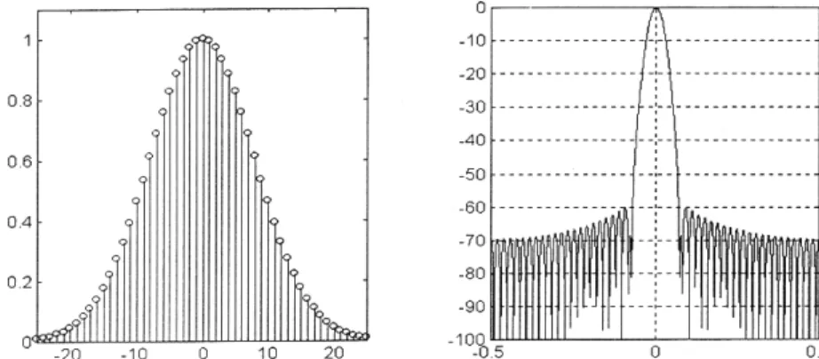
The time and frequency responses of the win- dows listed in Table-1 are presented in figures 4 through 9. The windows contain 51 -samples, a length selected to permit us to see some detail in their (1024) point Fourier Transforms. The appar- ent modulation of the spectral side-lobes is an artifact due to the sampling grid bracketing the spectral zero-crossings.
4. WINDOWS WITH ADJUSTABLE DESIGN PARAMETERS We recognize that windows trade spectral main- lobe width for spectral side-lobe levels. A good window achieves low side-lobe levels with mini- mum increase in main-lobe width. We now exam- ine two windows that can make this trade in accord with an optimality criterion.
4.1 Dolph-Tchebyshev Window The optimality criterion addressed by the Dolph- Tchebyshev window is that its Fourier transform exhibit the narrowest main-lobe width for a spec- ified (and selectable) side-lobe level. The Fourier transform of this window exhibits equal ripple at the specified side-lobe level. The Fourier Transform of the window is a mapping of the N- th order algebraic Tchebyshev polynomial to the N-th order trigonometric Tchebyshev polynomial by the relationship TN(X) = COS(Nq). The Dolph- Tchebyshev window is defined in terms of uni-
formly spaced samples of its Fourier Transform.
These samples are defined in (8).
Since the Discrete Fourier Transform is periodic on the unit circle, there is an end point problem with the sample located at pi when the unit circle is cut at pi. This requires a slight modification of the relationship shown in (8). This modification is shown in the MATLAB code presented below.
This code accomplishes the following tasks. First, reduce the number of sample points by one (from N to N-l). Second, compute N-l spectral samples.
Third, scale the first point by half and appends a copy of this scaled sample to the opposite end of the spectral array thus returning the array to the desired length N. Last, transform spectral samples to the time domain by an N-point DFT. This code is slightly simpler than me MATLAB code (Chebwin) used by the Signal Processing Toolbox and does not have the restriction that the size N be an odd integer.
function w=dolph(n,a)
%written by fred harris, SDSU n=n-1;
beta=cosh(acosh(10^(abs(a)/20))/n);
arg=beta*cos(pi*(0:n-1)/n);
wf=cos(n*acos(arg));
w=real(fft((wf.*cos(pi*(0:n-1)))));
w(1)=w(1)/2; w=[w w(1)];
w=w/max(w);
The Fourier Transform of this window exhibits uniform, or constant level side-lobes levels (inher- ited from the Tchebyshev polynomial) and as such must contain impulses in its time series.
These impulses are located at the window bound- aries. When this window is used as a shading function in antennae systems these impulses are not realizable and their suppression results in an allied window known as the Taylor weighting.
Figures 10 and 11 present the time and frequency description of a 40 dB side-lobe and an 80 dB side- lobe Dolph-Tchebyshev window. The 40 dB win- 1
0 )] :
( cosh cosh[
)) cos(
( cosh cosh
) 1 ( )
( 1
1
−
<
≤
−
= −
−
N N k
N N k
k
W k
β π β
where β is defined by:
)]
10 ( 1 cosh
cosh[ 1 A/20 N
−
= −
β
and where A=Sidelobe Level (in dB)
∑
−=
= 1
0
2
) ( )
( N
k
Nnk
ej
k w n
w
π
: and where W(N-k) = W(-k) (8)
dow is included to demonstrate the end point impulses. As an aside, the Tchebyshev, or equal ripple behavior of the Dolph-Tchebyshev window can be obtained iteratively by the Remez (or the Equal-Ripple or Parks-Mclellan) Filter design rou- tine. For comparison, figure 12 presents a window designed as a narrow-band filter with 60 dB side- lobes. The MATLAB call for this design was
ww=remez(50,[0 .001.047 0.5]/0.5,[11 0 0]).
The weights were scaled by ww(max) to set the maximum value of the window to unity. This fil- ter, by virtue of the equal-ripple side-lobes, also exhibits end point impulses.
A comment on system performance is called for at this point. Windows (and filters) with constant level side-lobes, while optimal in the sense of equal ripple approximation, are sub-optimal in terms of their integrated side-lobe levels. The window (or filter) is used in spectral analysis to reduce signal bandwidth and then sample rate.
The reduction in sample rate causes aliasing. The spectral content in the side-lobes, (the out-of band energy) folds back to the in band interval and becomes in-band interference. A measure of this unexpected interference is integrated side-lobes which, for a given main-lobe width, is greater when the side-lobes are equal-ripple. From a sys- tems viewpoint, the window (or filter) should exhibit 6-db per octave (1/0 rate of falloff of side- lobe levels. Faster rates of falloff actually increase integrated side-lobe levels due to an accompany- ing increase in close-in side-lobes as the remote side-lobes are depressed (while holding main- lobe width and window length fixed). System designers should shv awav from equal-ripple windows (and filters).
4.2 Gaussian window A second window that exhibits a measure of opti- mality is the Gaussian or Weierstrass function. A desired property of a window is that they be
smooth (usually) positive functions with Fourier Transforms which approximate an impulse, (i.e.
tall thin main lobe with low level side-lobes).
From the uncertainty principle we know that we cannot simultaneously concentrate both a signal and its Fourier Transform. We can define the measure of concentration (or width) as the func- tion's second central moments (i.e. moment of inertia). With sT being the RMS time duration and with sw being the RMS bandwidth (in Hz.) we know these parameters must satisfy the uncer- tainty principle inequality shown in (9).
The equality constraint is achieved only by the Gaussian function. Thus the Gaussian function, exhibiting a minimum time-bandwidth product, seems like a reasonable candidate for a window.
Since windows span a finite support, when the Gaussian is used as a window we must truncate or discard its tails. By restricting the window to a finite support the (truncated) Gaussian loses its minimum time-bandwidth distinction. Never-the- less, the window enjoys wide usage by virtue of its simplicity and (misplaced) reputation as a minimum time-bandwidth function. The sampled Gaussian window is defined in (10) with the parameter a, the inverse of the standard devia- tion, controlling the effective time duration and the effective spectral width.
The sampled Gaussian window is defined in (10) with the parameter a, the inverse of the standard deviation, controlling the effective time duration and the effective spectral width.
The Fourier Transform of this truncated window is the convolution of the Gaussian transform with a Dirichlet kernel as indicated in (11). The convo- lution results in the formation of the spectral
2
≥ 1
W Tσ
σ (9)
− +
2
2 / 2 exp 1 )
( N
n n
w α
(10)
main-lobe (approximating the target's main-lobe) with accompanying side-lobes whose peak levels depend on the parameter a. As expected, larger a leads to wider main-lobe and lower side-lobes.
Figures 13 and 14 present Gaussian windows with parameter a selected to achieve 60 and 80 dB side- lobe levels. Note that the main-lobes are consider- ably wider that those of the Dolph-Tchebyshev and the upcoming Kaiser-Bessel windows. A use- ful observation is that the main-lobe of the Gaussian window is 1/3 again wider than the Blackman-harris window exhibiting the same side-lobe level.
4.3 Kaiser-Bessel Window The last window we examine, designed in accord with an optimality criterion, is the Kaiser-Bessel (or Prolate Spheroidal Wave Function). The previ- ous two windows were characterized by mini-
mum main-lobe width for a.given side-lobe level and (hopefully) minimum bandwidth by approx- imately a minimum time-bandwidth product.
Both windows had defects; one exhibited constant level sidelobes (resulting in high integrated side- lobes), the other exhibited excessive main-lobe width. An alternate, and related, optimality crite- rion is the problem of determining the wave- shape on a finite support that maximizes the ener- gy in a specified bandwidth. This wave-shape has been identified by Slepian, Landau, and Pollak as the Prolate Spheroid function (of order zero) which contains a selectable time-bandwidth product parameter. Kaiser has discov- ered a simple numerical approximation to this function in terms of the zero- order modifed Bessel function of the first kind (hence the designation Kaiser- Bessel). The Kaiser-Bessel
window is defined in (11) where the parameter pa. is the window's half time- bandwidth product. The series for the Bessel function converges quite rapidly due to the k! in the denominator.
The transform of the Kaiser-Bessel win- dow is (within very low level aliasing terms) the function shown in (12), We see that this function tends to sinx/x when the spectral argument is evaluated beyond the time-bandwidth related main-lobe bandwidth.
Note that the Caiser-Bessel window can also be approximated by samples of the main-lobe of its spectra since the win- dow is self-replicating under the tune- limiting and band-limiting operations.
Figure 13. Gaussian (60 dB, α=3.1) window and its Fourier Transform
Figure 14. Gaussian (80 dB, α=3.7) window and its Fourier Transform
[ ]
παπα
0
0 1.0 /2
)
( I
N I n
n
w
−
= where
2
0
0 !
) 2 / ) (
(x =
∑
k∞= xk kI
(11)
That is if w(n) and W(θ) are a Fourier Transform pair, then the band-limited version Rect(θ/απ)- W(θ) is a scaled version of (the envelope of) w(n) and the transform of theband-limited spectra is a time series consisting of the original time-limited seriesw(n) with appended side-lobe tails. Time limiting this new time series (truncating the tails) returns the pair back to their original relationship.
Figures 15 and 16 present the Kaiser-Bessel win- dow for parameter ap selected to achieve 60 and 80 dB side-lobes. Compare the main-lobe widths to those of the earlier windows. As commented upon earlier, windows can be designed using the Remez Algorithm. When the penalty function of the Remez algorithm is made to increase linearly with frequency the side-lobes fall inversely with frequency (-6 dB/oct). Figure 17 presents a win- dow designed by a modified Remez algorithm.
The call to the modified routine is of the form
Note that due to the reduced sidelobe slope this window exhibits a narrower main-lobe width compared to a Kasier-Bessel with the same -80 dB side-lobe level.
5. SPECTRAL ANALYSIS AND WINDOW FIGURES OF MERIT Windows are used in spectrum analysis to mini- mize additive biases caused by the artificial boundaries or discontinuities imposed on the time series being analyzed. We will now examine the incidental effects of the windows on the spec- trum analysis process. In one use of a spectrum analyzer, we process a composite signal consist- ing of a sinusoid of interest, which we will con- sider the desired signal, other sinusoids, not of
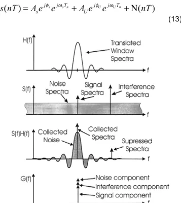
interest which we will consider undesired inter- ference, and additive white noise. Figure 18 is a
representation of the spectra of this signal set containing a single unde- sired line component, the signal described in (13).
The primary signal processing tool used to per- form spectrum analysis is the Discrete Fourier Transform (DFT). Consequently we will limit sub- sequent discussion of windows in spectral analy- sis to DFT based analysis. The DFT of the com- posite signal described in (13) will consist of three components as shown in figure 18 and as present- ed in (14). In this expression 5k and Ak are the fre- quency displacements (in DFT bins) of the desired and undesired signal components from the DFT bin closest to the desired signal frequen- cy. Recall that the DFT bin centers are located at integer multiples of the fundamental frequency 2π/NT radians/second defined by the support interval NT. Thus sampled data frequency is defined by the index k with units of cycles per
( ) [ ( ) ]
( )
2 22 2
0 ( /2)
) 2 / ( ) sinh
( απ θ
θ απ
θ απ
N N I
W N
−
= −
(12)
ww=remez(50,[0.001.0655 0.5]/0.5,|1 1 0 0],'slope = -1').
) ( )
(nT Ae e A e e nT
s = s jφs jωsTn + U jφU jωUTn +Ν
(13)
Figure 18. Graphical Representation of Spectra Interacting With Observation Window
interval or by the equivalent sampled data fre- quency of k(2π/N) radians/sample.
The three separate components of the DFT pre- sented in (14) are identified and shown in (15).
The signal component, S(k)DES SIG. of the DFT out- put is seen to preserve the complex amplitude of the input sinusoid but multiplies that amplitude by a gain term we recognize as the DFT of the window. The DFT is evaluated at δk. the frequen- cy displacement of the input sinusoid from the nearest DFT bin. We note that the frequency response of the window spectra centered at the k- lh bin and observed by the input sinusoid at fre- quency k+δk cvcles/interval is the same as the frequency response of the window centered at DC and observed at frequency offset δk. When the displacement, dk, is zero this gain defaults to the DC (or zero frequency) response of the window.
This gain is called the peak amplitude gain of the window and as shown in (16) is the sum of the
window weights. This sum is bounded by N (for the rectangle window) and is aoN for the short cosine transforms presented in sec- tion 3. For good windows, typical val- ues of peak amplitude gain is on the order of 0.5*N through 0.35*N. A related gain term is called the peak power gain of the window which is also shown in (16).
The undesired component, S(k)UNDES SIG, of the DFT output is also seen to preserve the complex amplitude of the input sinusoid but multiplies that amplitude by a gain term W(Dk). We recog- nize the gain term as the DFT of the window eval- uated at Dk, the frequency displacement of the undesired input sinusoid from the DFT bin of interest. This term is the spectral leakage term or out-of-band frequency response of the window. It is our desire to control this term that motivated us to design and use good windows. When Dk is greater than the window's main-lode width (3-to- 6 bins) this term is the window's side-lobe levels which can be on the order of 0.01 *N through 0.0001 *N.
The component S(k)NOISE is the DFT of the input noise. We can assume that this noise-is zero mean and white with variance σ2N. Since the noise in a random variable, so is it's DFT, so we are obliged to describe the DFT of the noise by its statistics.
Two statistics of primary interest are, as shown in (17), the first and second moments.
We see that the DFT output variance, due to input noise, is a scaled version of the input noise vari- ance. The scale term is the sum of square of the window weights. This gain, shown in (18) is termed the peak noise power gain of the window.
This of course is bounded by N (for the rectangle)
∑
=− −= 1
0
2
) ( ) ( )
( N
n
Nnk
e j
n s n w k
S
π
Nnk j k
k Nn u j j u k k Nn N j
n
S j
Se e Ae e N n e
A n w
π ϕ π
π δ ϕ
) 2 2 ( )
2 ( 1
0
)]
( )[
( + + + +∆ −
−
=
+ +
=
∑
(14)Nnk j k k Nn s j N j
N
s
DESSIG w n Ae e e
k S
δ π
ϕ 2π ( ) 2
1
0
) ( )
( − + + −
∑
==
=Asejφs
∑
Nn=−01w(n)ej2Nπnδk= AsejφsW(δk)
Nnk j k k Nn u j N j
N
u
UNDESSIG w n Ae e e
k
S π π
ϕ 2 ( ) 2
1
0
) ( )
( − + +∆ −
∑
==
= AUejφU
∑
Nn=−01w(n)ej2Nπn∆k=AUejφuW(∆k)
Nnk N j
N
NOISE w n n e
k S
π 1 2
0
) ( ) ( )
(
− −
∑
= ℵ=
(15)
Peak Signal Gain≡W(0)=
∑
Nn=−o1w(n)Peak Signal Power Gain≡W2(0)=
[ ∑
Nn=−o1w(n)]
2(16)
and is on the order of (3/8) N for other windows.
5.1 Figures of Merit The use of a window leads to conflicting effects on the output of the transform. The window is applied to data to suppress out-of-band side-lobe levels: this is a desirable effect. The window con- trols side-lobes by smoothly discarding data near the boundaries of the observation interval. This has the effect of reducing the amplitude, hence energy, of both signal and noise components pre- sented to the transform. Concurrently, the increased bandwidth of the window's spectral main-lobe (required to purchase the reduced side- lobe levels) permits additional noise into the measurement.
To facilitate comparison of different windows we define two performance measures related to the effects of the window on both signal and noise.
The first of these is equivalent noise bandwidth (ENBW). This parameter indicates the equivalent rectangular bandwidth of a filter with the same
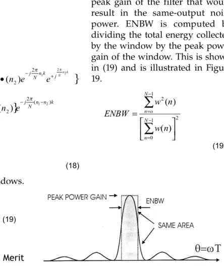
peak gain of the filter that would result in the same-output noise power. ENBW is computed by dividing the total energy collected by the window by the peak power gain of the window. This is shown in (19) and is illustrated in Figure 19.
We note that the rectangle window has the small- est ENBW of 1/N while a Hann window has an ENBW of 1.5/N. The units of ENBW is spectral bins, and larger ENBW indicates an increased variance of a spectral measurement. It is common practice to normalize the ENBW of the particular window of length N to the ENBW of the rectangle of the same length. Thus the normalized ENBW of the Harm window is 1.5 bins A table of popu- lar windows along with their ENBW is presented at the end of this section.
A related figure of merit for a windowed DFT is the Processing Gain (PG) or improvement in sig- nal-to-noise ratio obtained when using the win- dow. This improvement is the ratio of output SNR to input SNR of a noisy sinewave. Processing Gain can be as large as N (for a rectangle) and is usual- ly on the order of 0.4N for windows with good
{ }
ℵ
=
∑
−= 1 − 0
2 )
( N ( ) ( )
n
jN k
NOISE E w n n e nk
S E
π
nk e
n n w
N
n
jN
∑
=− ℵ −= 1
0
2
) ( ) (
π
=0
{ }
N jNnk jNnk}
n N
n
NOISE k E w n w n n n e e
S
E 2
2 1
1 2
2 2 1
2 1
0 1
0 1
2 ( ) ( ) ( ) ( )
) (
π π
− +
−
=
−
=
• ℵ ℵ
•
=
∑ ∑
{ }
jN n n kN
n N
n
e n n E n w n
w ( )
2 2 1 2
1
0 1
1
0 1
2 1
2
) ( ) ( ) ( )
( − −
−
=
−
= • ℵ ℵ
=
∑∑
π1 2 0 1
2( ) ℵ
−
∑
== N w nσ
n
) (
1
0 1 2 2
n w
N
n
∑
−ℵ =
=σ (18)
Peak Noise Power Gain 1 ( )
0 2 n w NPG N
n
∑
−=
=
≡
(19)
1 2
0
1 2
) (
) (
=
∑
∑
−
=
−
= N
n N
o n
n w
n w ENBW
(19)
Figure 19. Equivalent Noise Bandwidth (ENBW): Area Under Power Gain Curve Allocated to Rectangle Of Same Amplitude
side-lobe levels. As shown in (20), the processing gain is also equal to the reciprocal of the win- dow's ENBW.
5.1.1 Scalloping Loss The amplitude gain of a windowed transform applied to a sinusoid located at bin k+δk was pre- sented in (16) and is repeated here in (21). The amplitude gain W(δk) is a function of the fre- quency offset, dk, of the input sinusoid from the processed bin. This frequency dependent gain
due to the offset from the DFT bin center repre- sents a reduction in processing gain and is known as scalloping loss. The structure of the frequency dependent gain can be visualized with the aid of figure 20.
As shown in figure 20, when a sinusoidal input frequency is located in the center of a particular DFT bin, the pair of filters bracketing this bin respond with equal amplitudes. If the center fre- quency of an input sinusoid is shifted from the
bin center of filter k towards filter k+1, the ampli- tude response of filter k-1 and filter k drops and the response of the filter k+1 is increased. This drop in amplitude is scalloping toss. When the sinusoid is located at the midpoint between two filters, say at k+1/2, the two bracketing filters, k and k+1, respond with the same amplitude. This amplitude corresponds to the maximum reduc- tion in filter response and is called the peak scal- lop loss. When Peak scallop loss is presented in dB, it represents the maximum reduction in signal to noise ratio of a windowed transform due to spectral position of input signals. Note that if the signal can never be located more than V2 a bin form some center frequency. The rectangle win- dow, due to its very narrow main-lobe width, exhibits the maximum scallop loss of-3.9 dB.
Windows with deeper side-lobe levels have wider main-lobes and consequently exhibit reduced scalloping loss typically on the order of 1.0 dB.
If scalloping loss is an important consideration, it can be significantly reduced by zero extending the windowed data and performing a double length transform. The loss then corresponds to a ¼ bin shift of the original spectral analysis. An alternate technique is to modify the window so that it is has a flat spectral width between bin centers. This modification of window criterion results in win- dows with negative weights and a significant increase in ENBW of the filter. We have used this form of a window, called the harris-flatop in a number of spectrum analyzers used as frequency dependent voltmeters (for use in acceptance test- ing procedures). The parameters of this window are presented in the figure of merit table and fig- ure 21 presents the time and frequency response of the window as well as a detailed view of its scallop loss
5.1.2 Overlap Correlation When the DFT is used to obtain power spectral estimates of random stationary processes an ensemble of spectral measurements are averaged
∑
∑
−
= ℵ
−
=
= 1
0 2 2
1 2
0
2 ( )
N
n N
n out
n w
n w A SNR
σ
= 2ℵ 2
σ SNRIN A
n ENBW w
n w SNR
PG SNR N
n N
n in
OUT ( ) 1
1
0 2 1 2
0 =
=
=
∑
∑
−
=
−
=
(20)
Nkn j n k N k s j N j
n
s
DESSIG k w n Ae e e
S π δ π
ϕ 2 ( ) 2
1
0
) ( )
( − + −
∑
==
N kn N j
o n s j
se w n e
A
πδ ϕ
1 2
)
∑
=− (=
) ( k W e As jϕs δ
= (21)
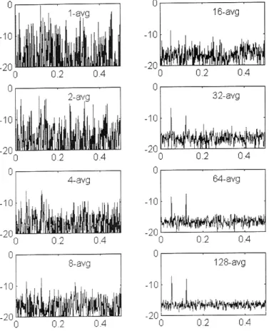
to reduce the variance of the estimates. When the successive transforms are obtained from non- overlapped segments of the time series, the stan- dard deviation of the spectral estimates obtained by simple averaging is reduced by the square-root of the number of averages. For instance, averaging 32 independent transforms will reduce the stan- dard deviation by a factor of 5.6 or 15. dB. Figure 23 demonstrates the improvement in variance obtained by the ensemble averaging of independ- ent transforms. We apply windows to data to sup- press artificial discontinuities at the data bound- aries. The window essentially discards the data in the intervals nears near the boundaries. To avoid missing data we overlap successive intervals and obtain what has been called the sliding windowed DFT. Typical values of interval overlap for succes- sive transforms is 75% and 50%. These overlap intervals are often called 4-to-l overlap and 2-to-l overlap respectively. The data collected from suc-
cessive overlapped and windowed trans- forms is not independent. Consequently, the degree of variance reduction obtained by ensemble averaging of spectra will be signif- icantly reduced.
The variance reduction obtained by averag- ing correlated data can be easily determined by examining the terms in the covariance matrix of the summation shown in (22).
When the entries in the summation of (22) are independent, the diagonal terms of the covariance matrix are the only non zero terms and the summation collapses to c(0)/N. When the collected data represents 50% overlapped intervals, The matrix becomes. banded and contains only the diag- onal terms and the first upper and lower off diagonal terms. Gathering all the terms on the three diagonals results in the summation shown in (23).
When the collected data represents 75%
overlapped intervals. The matrix becomes
banded and contains only the diagonal terms and the three upper and lower off diagonal terms.
Gathering all the terms on the seven diagonals results in the summation shown in (24).
Figure 21a. harris flattop window and its Fourier Transform
Figure 21b. Scallop Response of Three Adjacent DFT bins for -80dB Dolph-Tchebyshew window
]
∑−
=
= 1 ( )2
0
2 1 N p n
Nn AVG E
σ
+
− +
− +
−
−
−
−
−
0 ( ...
) 3 (
) 2 (
) 1 (
...(
) 0 ( )
1 ( )
2 (
( ...
) 1 ( )
0 ( )
1 (
( ...
) 2 ( )
1 ( )
0 ( 1
2
r N
r N
r N
r
N r
r r
N r r
r r
N r r
r r
N SUM
O O
O O
(22)
[
(0) 2 (0.5)]
2[
(0.5)]
) 1
% 50
(. 2
2 r
r N OL N
AVG − = + −
σ
(23)
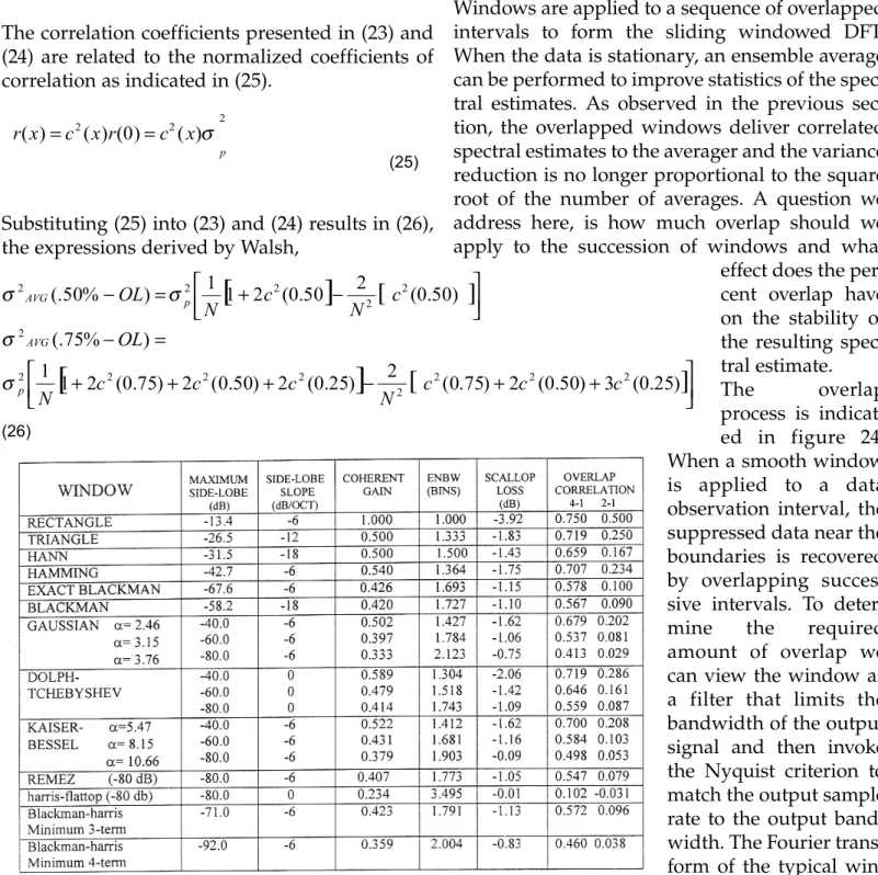
The correlation coefficients presented in (23) and (24) are related to the normalized coefficients of correlation as indicated in (25).
Substituting (25) into (23) and (24) results in (26), the expressions derived by Walsh,
The correlation coefficients required to evaluate (26) are listed in Table 2, For many useful win- dows
5.2 How Much Overlap?
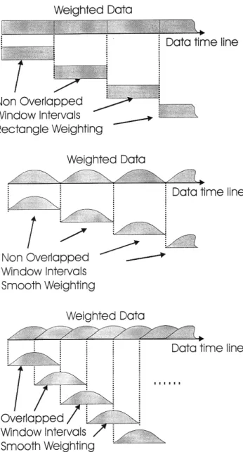
Windows are applied to a sequence of overlapped intervals to form the sliding windowed DFT.
When the data is stationary, an ensemble average can be performed to improve statistics of the spec- tral estimates. As observed in the previous sec- tion, the overlapped windows deliver correlated spectral estimates to the averager and the variance reduction is no longer proportional to the square root of the number of averages. A question we address here, is how much overlap should we apply to the succession of windows and what effect does the per- cent overlap have on the stability of the resulting spec- tral estimate.
The overlap process is indicat- ed in figure 24.
When a smooth window is applied to a data observation interval, the suppressed data near the boundaries is recovered by overlapping succes- sive intervals. To deter- mine the required amount of overlap we can view the window as a filter that limits the bandwidth of the output signal and then invoke the Nyquist criterion to match the output sample rate to the output band- width. The Fourier trans- form of the typical win- dow and the required
[ ]
[
(0.75) 2 (0.50)]
3 (0.25)2
25 . 0 ( 2 ) 50 . 0 ( 2 ) 75 . 0 ( 2 ) 0 1 (
)
% 75 (.
2 2
r r
N r
r r
r N r
OL
AVG
+ +
−
+ +
+
= σ −
(24)
2 2
2( ) (0) ( )
) (
p
x c r x c x
r = = σ
(25)
[ ] [ ]
+ −
=
− 2 (0.50)
50 . 0 ( 2 1 1 )
% 50
(. 2 2 2 2
2 c
c N OL p N
AVG σ
σ
[ ] [ ]
+ + + − + +
=
−
) 25 . 0 ( 3 ) 50 . 0 ( 2 ) 75 . 0 2 (
) 25 . 0 ( 2 ) 50 . 0 ( 2 ) 75 . 0 ( 2 1 1
)
% 75 (.
2 2
2 2 2
2 2
2 2
c c
N c c
c N c
OL
p AVG
σ σ
(26)
TAble 2. Figures of Merit for Common Windows
![Figure 21b. Scallop Response of Three Adjacent DFT bins for -80dB Dolph-Tchebyshew window ] ∑−==1()2021NpnNnAVGEσ +−+−+− −−−−0(.....)3()2()1(.....()0()1()2((.....)1()0()1((.....)2()1()0(12rNrNrNrNrrrNrrrrNrrrrNSUMOOOO (22) [ ( 0 ) 2](https://thumb-eu.123doks.com/thumbv2/1library_info/5310105.1678777/18.918.59.490.376.575/figure-scallop-response-adjacent-dolph-tchebyshew-npnnnavgeσ-rnrnrnrnrrrnrrrrnrrrrnsumoooo.webp)