Tracking Economic Activity With Alternative High-Frequency Data

Research Collection

Working Paper

Tracking Economic Activity With Alternative High-Frequency Data

Author(s):

Eckert, Florian; Kronenberg, Philipp; Mikosch, Heiner; Neuwirth, Stefan Publication Date:

2020-12

Permanent Link:

https://doi.org/10.3929/ethz-b-000458723

Rights / License:

In Copyright - Non-Commercial Use Permitted

This page was generated automatically upon download from the ETH Zurich Research Collection. For more

information please consult the Terms of use.

KOF Working Papers, No. 488, December 2020

Tracking Economic Activity With Alternative High-Frequency Data

Florian Eckert, Philipp Kronenberg, Heiner Mikosch and Stefan Neuwirth

ETH Zurich

KOF Swiss Economic Institute LEE G 116

Leonhardstrasse 21

8092 Zurich, Switzerland

Phone +41 44 632 42 39

Fax +41 44 632 12 18

www.kof.ethz.ch

kof@kof.ethz.ch

Tracking Economic Activity With Alternative High-Frequency Data

Florian Eckert

, Philipp Kronenberg

, Heiner Mikosch

, and Stefan Neuwirth

†

KOF Swiss Economic Institute, ETH Zurich

December 16, 2020

Abstract

Most macroeconomic indicators failed to capture the sharp economic fluctuations dur- ing the Corona crisis in a timely manner. Instead, alternative high-frequency data have been used, aiming to monitor the economic situation. However, these data are often only loosely related to the business cycle and come with irregular patterns of missing observations, ragged edges and short histories. This paper presents a novel mixed- frequency dynamic factor model for measuring economic activity at high-frequency intervals in rich data environments. Previous research has estimated the dynamic factor conditional on actually observed data only. In contrast, we propose to estimate the dynamic factor conditional on a balanced panel with observed and latent data information, where the latent data are themselves estimated in a separate state-space block. One benefit of this data augmentation strategy is that it allows to easily ac- count for serial correlation in the factor measurement errors. We apply the model to a set of daily, weekly, monthly and quarterly series and extract a dynamic factor, which is identified as the weekly growth rate of GDP. It turns out that the model is well suited to exploit the business cycle information contained in alternative high- frequency data. GDP is tracked timely and accurately during the Corona crisis and past economic crises.

JEL Classification: C11, C32, C38, C53, E32, E37

Keywords: Economic Activity Indicator, Real Time, Nowcasting, Alternative High- Frequency Data, Mixed-Frequency Dynamic Factor Model, Data Augmentation

∗

Corresponding author: ETH Zurich, Leonhardstrasse 21, Building LEE, 8092 Zurich, Switzerland,

e-mail: mikosch@kof.ethz.ch, phone: +41 44 632 42 33, fax: +41 44 632 12 18

1 Introduction

The Corona crisis has shaken many economies worldwide to an unprecedented extent.

Economic activity fell dramatically within a few days and rebounded very quickly after the first wave of lockdowns ended. Macroeconomic indicators, such as business tendency surveys, consumer sentiment, retail sales or industrial production, could not keep track of the sudden fluctuations. Most of these variables are released only once a month and with a publication lag, making them not well suited to capture the dynamics in a timely man- ner. Instead, business cycle observers started to use various high-frequency series such as daily credit card transactions, energy consumption, traffic volumes, smartphone mobility tracking and internet search hits, with the aim of monitoring economic activity closer to real time. Henceforth, we refer to these series as alternative high-frequency data, a term which is increasingly common since the outbreak of the crisis. However, the real-time monitoring task is challenging due to the characteristics of the alternative high-frequency data. Some of the series are only loosely related to economic activity as measured by sta- tistical offices. Others cover only very specific aspects of economic activity. In addition, the series often fluctuate strongly and are affected by factors unrelated to the business cycle. Furthermore, most of them have only a short history and are subject to irregular patterns of missing observations and publication lags.

Against this background, we propose a novel mixed-frequency dynamic factor model (DFM) which is well suited to measure GDP growth at high-frequency intervals and close to real time and to extract the business cycle information contained in alternative high- frequency data, despite their aforementioned challenges. Our DFM accounts for stochastic volatility and for serial correlation in the factor measurement errors. It comprises three in- terdependent state-space blocks: latent high-frequency data, dynamic factor and stochastic volatility. In the first block, all unobserved data points in the mixed-frequency data set are estimated as latent states conditional on, among others, the actually observed data and temporal aggregation constraints. In the second block, the dynamic factor is estimated conditional on, amongst others, the observed as well as the estimated latent information.

The strategy of creating a balanced data set through estimation of unobserved informa- tion as latent states is known as data augmentation in the statistics literature (Tanner and Wong, 1987; Frühwirth-Schnatter, 1994). We take a fully Bayesian approach to estimate the latent information, the dynamic factor, the stochastic volatility and all model param- eters. The joint posterior is simulated using Gibbs sampling.

The literature on mixed-frequency DFMs has seen important advances during the past years (e.g., Giannone et al., 2008; Aruoba et al., 2009; Camacho and Perez-Quiros, 2010;

Doz et al., 2011; Bańbura et al., 2011; Bańbura and Modugno, 2014). However, the han-

dling of data sets with several mixed frequencies, with a large set of daily and weekly series,

with arbitrary and irregular patterns of missing observations and with data histories of

varying lengths remains a challenge. Here, our paper provides several novel contributions.

To begin with, previous models estimate the dynamic factor by modifying the Kalman filter recursions such that they skip the updating step if observations are missing. In con- trast, our model estimates the dynamic factor not just based on actually observed data only, but also conditional on the latent information contained in the data set. For this, we integrate a novel state-space block into the DFM, in which the sparse observed data points in the mixed-frequency data set are augmented to a balanced panel with observed and estimated latent information. An important advantage of creating the balanced panel in the data augmentation block is that it allows for quasi-differencing of the dynamic fac- tor measurement equation (Chib and Greenberg, 1994). Thereby, the model can easily account for serial correlation in the factor measurement errors despite mixed frequencies, missing observations, different release lags and data histories of various different lengths in the original data. This feature is crucial since it allows the common factor to have less explanatory power for the mixed-frequency series during extended periods of time while explaining a lot during other periods (e.g., Stock and Watson, 2002). This, in turn, can greatly improve the performance of DFMs, especially when alternative high-frequency data with the aforementioned characteristics are used. Previous papers obtain the condi- tional moments of the serially correlated measurement errrors from the Kalman smoother, typically using an EM-algorithm, which increases the computational burden substantially (e.g., Bańbura and Modugno, 2014). In contrast, we provide an efficient and generic Bayesian sampling algorithm that scales well to larger data sets. In order to estimate the latent high-frequency data, the dynamic factor and the stochastic volatility, we build on the precision sampler framework developed by Chan and Jeliazkov (2009). Our novel contribution here is to extend their procedure to the mixed-frequency case by integrating the temporal aggregation scheme originally proposed by Mariano and Murasawa (2003).

This leads to substantial efficiency gains compared to forward filtering backward sampling (Carter and Kohn, 1994; Kim and Nelson, 2017), in particular when dealing with the large state-space setups required for mixed- and high-frequency data. Another advantage of our approach is that the dynamic factor resulting from the model estimation has a clear and intuitive interpretation. In particular, we propose straightforward identifying restrictions such that the common factor extracted from a mixed-frequency data set can be interpreted as the high-frequency period-on-period growth rate of GDP.

In an empirical application, we study how useful the DFM is for tracking Swiss GDP

with a large set of daily, weekly and monthly time series, including various alternative

high-frequency data. We derive a weekly economic activity indicator that is identified as

week-on-week GDP growth. A pseudo real-time analysis yields that the indicator is able

to capture business cycle turning points comparatively early. It tracks economic activity

well during times of sudden and strong economic fluctuations such as the Great Reces-

sion in 2008/09, the European sovereign debt crisis in 2011 and the Swiss franc shock in

2015. An in-depth investigation is provided for the Corona crisis, where the weekly GDP

indicator performs especially well due to the information extracted from the alternative high-frequency data.

Further, we conduct a pseudo real-time out-of-sample nowcast ex- ercise for quarterly GDP. The mixed-frequency DFM substantially outperforms simple benchmark models. The alternative high-frequency data turn out to be especially useful for nowcasting GDP during sharp economic downturns and recoveries as compared to us- ing macroeconomic and financial series only. In contrast, the alternative high-frequency data do not provide additional valuable information during normal times.

The remainder of the paper is structured as follows. Section 2 presents the mixed-frequency DFM with stochastic volatility, where special emphasis is put on the discussion of the data augmentation part. The section further describes the identifying assumptions and discusses our estimation priors. In addition, a description of the sampling algorithm is provided. Section 3 presents the results from the empirical application, including a description of the employed data. Section 4 concludes.

2 Mixed-Frequency DFM with Data Augmentation

2.1 Data Augmentation

The model uses a collection of n time series with mixed frequencies, where the time index of the highest frequency in the data set is denoted by t. In order to coerce all time series to the highest frequency, low-frequency observations are registered in the last high-frequency entry of the corresponding low-frequency period and all other entries are filled with zeros.

For instance, when mixing weekly, monthly and quarterly data, monthly (quarterly) data are observed in the last week of each month (quarter) and are set to zero elsewhere. A time series is also assigned a value of zero in a period if the observation is missing due to publication delays or a limited history. The n-dimensional data vector y

is, therefore, typically filled with a few observations and many zeros. Further, we define x

as an n- dimensional vector filled with actual observations and with estimated latent observations whenever a variable is not observed. The relation between the sparse vector y

and the dense vector x

is described by the following identity:

y

= S

x

, (1)

where S

is a diagonal selection matrix of order n × n, featuring ones on the diagonal if the corresponding value in y

is observed and zeros otherwise. Henceforth, we refer to the strategy of augmenting the sparse vector y

to the dense vector x

, which contains observed and estimated data, as data augmentation. Consequently, Equation (1) is referred to as

1

We would like to highlight other recent projects that employ alternative high-frequency data to track the

economy during the Corona crisis. Lewis et al. (2020) provide a weekly economic activity indicator for

the United States using both a principal components and a dynamic factor approach. Eraslan and Götz

(2020) do so for Germany taking a principal components approach. For Switzerland, Eckert and Mikosch

(2020) present daily activity indicators and Guggia et al. (2020) present a weekly economic activity index.

the data augmentation equation. As will be seen in the next subsection, data augmentation enables us to easily account for serial correlation in the measurement errors of a mixed- frequency DFM.

2.2 Dynamic Factor

The measurement equation for the dynamic factor f

is given by

x

= L

λf

+ L

λf

+ . . . + L

λf

+ e

. (2)

where s indicates the number of factor lags, the n-dimensional vector λ contains the time-invariant factor loadings and the diagonal distributed lag matrices L

, . . . , L

ensure the appropriate temporal aggregation of the high-frequency factor to the lower frequency variables in x

, as proposed by Mariano and Murasawa (2003) (see Appendix A.1 for details). The measurement errors in Equation (2) follow the first-order autoregressive process

e

= ρe

+ u

u

∼ N (0, Σ) (3)

with the error covariance matrix Σ and the autoregressive coefficient matrix ρ being diagonal. In order to estimate the dynamic factor in presence of serial correlation in the measurement errors, we follow Chib and Greenberg (1994) and quasi-difference the measurement equation. For this, we first define the quasi-differenced augmented data vector as

˜

x

= x

− ρx

. (4)

Inserting Equation (2) into Equation (4) yields the quasi-differenced measurement equation for the dynamic factor:

˜

x

= L

λf

+ . . . + L

λf

− ρ L

λf

+ . . . + L

λf

+ u

, (5) where u

has been defined in Equation (3) and is serially uncorrelated.

Notably, the elimination of serially correlated measurement errors via quasi-differencing is only possible because the original measurement equation given in Equation (2) includes the dense data vector x

. In contrast, elimination of serially correlated measurement errors by quasi- differencing is not possible when the measurement equation includes the sparse data vector y

. Thus, the data augmentation from y

to x

is a necessary step to account for serial correlation in the measurement errors. The state equation for the dynamic factor is given by the autoregressive process

f

= φ

f

+ . . . + φ

f

+ e

η

, η

∼ N (0, 1) (6)

2

It is straightforward to rearrange terms in Equation (5) to simplify the estimation of the factor.

where the scalars φ

, . . . , φ

represent the autoregressive coefficents and p indicates the number of lags. The composite error term e

η

consists of the time-varying stochastic volatility factor e

and the standard normally distributed error η

. Note that the state equation is not affected by the transformation from the original to the quasi-differenced measurement equation. Also, this transformation does not affect the measurement and the state equation for the stochastic volatility discussed in the next section.

2.3 Stochastic Volatility

We let the variance of the error term in Equation (6) be time varying in order to better capture volatility increases during crisis periods. Specifically, the logarithmized stochastic volatility factor follows the random walk process

h

= h

+ v

, v

∼ N (0, ω) (7)

which gives us the state equation of the stochastic volatility factor. Since solving Equa- tion (6) for h

would result in nonlinearities, we follow Primiceri (2005) and transform the equation to a linear system by squaring and taking logarithms. This results in the following measurement equation for the stochastic volatility factor:

log (f

− φ

f

− . . . − φ

f

)

+ c = 2h

+ log η

, (8) where the offset constant c = 0.001 is introduced to make the estimation more robust.

Since η

follows a standard normal distribution, the error term log η

is distributed according to a log chi-squared distribution with one degree of freedom, log χ

(1). In order to transform the system further to a Gaussian state-space model, the χ

(1)-distribution is approximated using a mixture of normals following Kim et al. (1998). Appendix A.2 provides further details.

2.4 Latent Data

The measurement equation for the latent dense data vector x

is given by

y

= S

x

+

,

∼ N (0, I

) , (9)

where = 10

is a very small number. This approximates the identity given in Equa- tion (1) very closely. Imposing an exact identity is not feasible, as the covariance matrix needs to be invertible in the precision sampling approach that we employ for estimation.

The state equation for x

is simply obtained by combining Equation (5) and Equation (4) to

x

= L

λf

+ . . . + L

λf

− ρ L

λf

+ . . . + L

λf

+ ρx

+ u

, (10)

where again u

∼ N (0, Σ).

2.5 Factor Identification and Interpretation

Since both the dynamic factor and the factor loadings are unknown, there exist infinite possibilities to explain the data. This is commonly referred to as observational equiva- lence. Therefore, in order to identify the factor, certain restrictions have to be placed on the parameter space. Following Bai and Wang (2015), the factor loading on GDP, denoted as λ

, is restricted to unity using informative priors. This resolves the scale and sign indeterminacy inherent in dynamic factor models. Rotational indeterminacy is not an issue in the single factor case (see, e.g., Aßmann et al., 2016, and references therein) and the dynamic factor is, therefore, uniquely identified.

One benefit of our approach is a clear and intuitive interpretation of the dynamic factor.

This is achieved by imposing informative priors such that the dynamic factor is equal to the high-frequency growth rate of GDP and that the temporal aggregation of the dynamic factor, given in Equation (2), approximates the quarterly growth rate of GDP. Specifi- cally, we shrink the autoregressive coefficient ρ

strongly towards zero. In addition, we shrink the error term σ

on GDP growth towards a small value. This value determines how much the temporally aggregated high-frequency factor is allowed to deviate from the observed GDP growth rates. It should be noted, that the shrinkage is neither necessary to achieve identification nor is it in any way inherent to our model itself. Other choices are possible depending on what the researcher wants to do with the model.

The priors on all remaining parameters are left completely uninformative. It leads to a more robust convergence, especially around turning points, when imposing additional stationarity constraints on the autoregressive coefficients of the dynamic factor. A detailed account of the conditional distributions is given in Appendix A.5.

2.6 Estimation

The estimation task comprises the estimation of the dynamic factor f

, the stochastic

volatility factor h

, the latent dense data vector x

as well as the parameters λ, φ

, . . . , φ

,

ρ, ω and Σ. The joint posterior distribution is simulated using Gibbs sampling. f

, h

, x

and the aforementioned parameters are estimated in separate Gibbs sampling blocks, con-

ditional on the observed data y

, the selection matrix S

and the distributed lag matrices

L

, . . . , L

. Sparse matrix preallocation and the use of sparse matrix algorithms make the

estimation computationally efficient. A set of starting values is randomly generated from

uniform distributions to ensure robust convergence of the sampler. We assess convergence

of the Gibbs sampling algorithm using trace plots and by checking differences in the recur-

sive means of selected parameters. Due to the parsimonious parameterization, a burn-in of

1,000 iterations is sufficient to achieve convergence. After convergence is achieved, another

1,000 draws are saved and evaluated.

For the estimation of f

, h

, x

in the separate Gibbs sampling blocks, we build on the procedure proposed by Chan and Jeliazkov (2009). We extend the algorithm to the case of mixed-frequency data by integrating the temporal aggregation scheme of Mariano and Murasawa (2003) into the procedure. The rest of this section explains the estimation of f

, while Appendices A.3, A.4 and A.5 describe the estimation h

, x

and the remaining parameters λ, φ

, . . . , φ

, ω, ρ and Σ, respectively.

To estimate f

, the measurement equation for the factor shown in Equation (5) is stacked over all time periods t = 1, . . . , T to get

x ˜ = Gf + u, u ∼ N (0, I

⊗ Σ) (11)

where

˜ x

n(T−1)×1

=









 x ˜

.. .

˜ x











, G

n(T−1)×(T+s)

=











−ρL

λ (L

− ρL

)λ . . . (L

− ρL

)λ L

λ

. .. . ..

−ρL

λ (L

− ρL

)λ . . . (L

− ρL

)λ L

λ









 .

Note that G integrates the temporal aggregation scheme of Mariano and Murasawa (2003) into the procedure of Chan and Jeliazkov (2009). The state equation for the factor given in Equation (6) is stacked correspondingly:

Hf = v, v ∼ N (0, V) (12)

where

H

(T+s)×(T+s)

=

























 1

−φ

1 .. . . .. ...

−φ

. . . −φ

1 . .. ... ... ...

−φ

. . . −φ

1



























, f

(T+s)×1

=

























 f

f

.. . f

.. . f

























 ,

and V is a diagonal matrix containing the time-varying variances e

, . . . , e

. The

precision matrix F

is then given by H

V

H and the conditional posterior of the factors

is normally distributed according to

f ∼ N (f

, F

) where f

= F

G

(I

⊗ Σ

)˜ x F

= F

+ G

(I

⊗ Σ

)G

.

This algorithm is computationally very efficient if block-banded matrix algorithms are used. Instead of inverting F

, it is faster to compute the banded Cholesky factor of F

and to solve for f

by forward and backward substitution.

3 Tracking GDP with Alternative High-Frequency Data

We want to know whether the mixed-frequency DFM is helpful for tracking economic activity. Our conjecture is that the model can be particularly useful during downturns and upturns, especially if they are very sharp as during the Corona crisis. For an empirical application, we assemble a set of mixed-frequency data on the Swiss economy and study the behavior of a weekly GDP indicator resulting from our model. Thereafter, we present a pseudo real time out-of-sample nowcast exercise for quarterly GDP growth.

3.1 Data

The employed data set includes 22 daily and one weekly series that can be classified as alternative high-frequency data. These data comprise diverse series such as, e.g., energy production and energy consumption volumes, the frequency of motor vehicles passing at important monitoring stations, the number of flight arrivals and departures at the main na- tional airport, debit and credit card transaction volumes in retail trade, the volume of cash withdrawals at ATM machines, and google search hits for the economic situation and for the purchase of consumption goods. A general challenge with alternative high-frequency data is that their history is often quite short. In fact, some of our series start in 2018 only or even later. Our model can easily deal with data sets where the series start at different dates or at a late stage during the nowcasting analysis. The reason is that each series is a latent process in vector x

of Equation (1), irrespectively of whether it is observed or not.

In addition to the alternative high-frequency series, the data set includes six daily and one

monthly financial series as well as 23 monthly macroeconomic series (labor market, price,

retail sale and business tendency survey variables). The set of financial and macroeco-

nomic variables is rather standard in the GDP nowcasting literature. We are interested

in knowing whether the alternative high-frequency data provide valuable information in

addition to the standard variables. Table 2 in Appendix A.6 provides an overview of all

series used in this paper, along with meta information such as frequency, starting date,

unit, transformation and source. Since our nowcasting exercise is conducted at a weekly

frequency, we aggregate all daily series in the data set to weekly frequency. A positive

side effect of the temporal aggregation is that weekly seasonality patterns in the daily series are circumvented. In order to ensure a regular frequency pattern of the time series, the aggregation is done such that each of the 12 months in a year consists of exactly four weekly observations, resulting in 48 weekly observations per year.

We carefully track the release dates of the weekly and monthly time series according to their release schedules of the year 2020. For the below real time analysis, only those ob- servations, which were actually available at a particular date, are employed as an input for the model. Table 2 reports the release lags of all variables in the data set. The weekly variables are released in the following week. The monthly variables are released in the first week of the following month, except the retail sales variables which get published with a delay of four weeks. Quarterly GDP is released with a lag of 9 weeks. The variable-specific release lags result in “ragged edges” in the data (Wallis, 1986), which our model can easily deal with.

Figure 11 in Appendix A.6 shows our target variable, the quarter-on-quarter growth rate of Swiss real GDP, adjusted for financial inflows and outflows stemming from international sport events. Since the year 2005, the Swiss economy has experienced four economic crises:

the Great Recession in 2008Q4–2009Q3, the European sovereign debt crisis in 2011Q3–

2013Q1, the Swiss franc shock in 2015Q1–2015Q2, and the Corona crisis in 2020Q1–

2020Q2.

It is debatable when exactly these crises started and ended. We simply choose the start and end periods of the crises such that they began with strong downturns of quarterly GDP and ended with strong upturns.

3.2 Weekly GDP Indicator

The dynamic factor resulting from our mixed-frequency DFM is constructed such that it approximately represents the annualized week-on-week growth rate of GDP (see Section 2.5). For this reason, we henceforth refer to the dynamic factor as weekly GDP indicator.

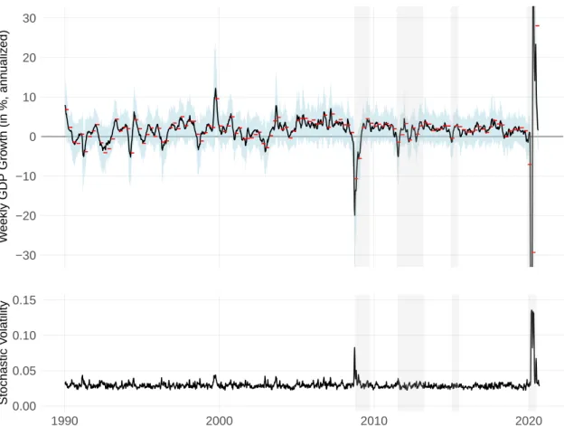
The upper panel of Figure 1 shows the weekly indicator and its 95%-confidence interval.

It is shown together with the actual quarter-on-quarter growth rate of GDP, indicated by horizontal red bars.

The weekly indicator and the quarter-on-quarter growth rate of GDP match well for the entire history. The lower panel shows the stochastic volatility of the errors in the state equation for the dynamic factor (see Equation (6)). Time-varying errors allow the factor to account for the higher volatility of economic activity during crisis periods. Indeed, we observe that the model makes use of this flexibility during periods of sudden and strong economic fluctuations, where the volatility of the error term increases.

3

Note to the editors and referees: 2020Q3 had not yet been published when the empirical part of the paper was finalized. We are happy to include the continuation of the Corona crisis in a revised paper version.

4

The unprecedented fluctuations during the Corona crisis eclipse the usual trajectory of weekly economic

activity. We cropped the vertical axis of the figure to allow for an inspection of the fluctuations during

other times. The Corona crisis will be discussed in greater detail later on.

−30

−20

−10 0 10 20 30

W eekly GDP Gro wth (in %, ann ualiz ed)

0.00 0.05 0.10 0.15

1990 2000 2010 2020

Stochastic V olatility

Figure 1: History of Weekly GDP Growth and Stochastic Volatility. The upper panel shows the dynamic factor, representing the annualized week-on-week growth rate of Swiss real GDP, together with a 95%-confidence interval in blue. The red bars depict the official annualized quarter- on-quarter growth rate of real GDP. The lower panel shows the estimated stochastic volatility.

Periods classified as economic crisis are indicated by vertical grey bars. The vertical axis of the upper panel is truncated to allow for an appropriate assessment of the entire history.

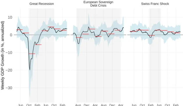
We conjecture that the previously presented alternative high-frequency data are especially useful in times of sharp and strong downturns and rebounds. They should capture the increased volatility faster and to a greater extent than traditional macroeconomic data.

To study this, we now put a special emphasis on the four economic crises in Switzerland

since the year 2005. We want to know whether the weekly GDP indicator is indeed able

to capture these sudden and strong economic fluctuations. Figure 2 presents the close-up

view of the weekly indicator together with 95%-confidence intervals (in blue) and with the

realized annualized quarter-on-quarter growth rate of GDP (in red). The crisis quarters

are indicated with vertical grey bars. During the Great Recession, the indicator shows

negative growth rates already at the beginning of August 2008, with a trough in mid-

November. From March 2009 onward, weekly growth turned positive again. The path of

the weekly growth rates reveals that both the downturn and the subsequent recovery were

very strong and abrupt, which cannot be captured by looking at quarterly or monthly fig-

ures only. During the European sovereign debt crisis, Switzerland experienced heightened

volatility over several quarters due to an appreciation of the Swiss franc, increased uncer-

tainty and very volatile transit trade. The weekly GDP indicator captures these ups and

downs quite well (see middle panel of Figure 2). On January 15, 2015, the Swiss National Bank unexpectedly removed the minimum exchange rate of 1.20 Swiss francs per euro.

This led to a rapid appreciation of the Swiss franc, which has become known as the “Swiss franc shock”. GDP declined by 0.7 percent in 2015Q1 and grew strongly again by 2.7 percent in the subsequent quarter. The weekly GDP indicator reveals that the economic downturn after the shock was relatively strong, but that a steep recovery started at the end of February already (see right panel of Figure 2). This prevented a more negative growth rate for 2015Q1. The indicator further reveals that economic activity was rather flat on average over the second quarter and that the strong quarterly growth rate was primarily due to a big statistical overhang stemming from the first quarter. Altogether, the analysis shows that the weekly GDP indicator can help to better understand rapid economic fluctuations after shocks.

Great Recession European Sovereign

Debt Crisis Swiss Franc Shock

Jun Oct Feb Jun Oct Feb Aug Dec Apr Aug Dec Apr Jun Oct Feb Jun Oct Feb

−30

−20

−10 0 10

W eekly GDP Gro wth (in %, ann ualiz ed)

Figure 2: Weekly GDP Growth During Crisis Periods. Notes: See Figure 1.

Next, we focus on the Corona crisis during which the Swiss economy, just as other

economies worldwide, experienced unprecedented fluctuations both in terms of sudden-

ness and strength. Figure 3 shows the weekly GDP indicator, again together with a

95%-confidence interval and with the actual quarter-on-quarter growth rate of GDP. The

vertical dotted lines indicate important policy decisions during the pandemic. The first

Corona virus infection was recorded on February 25, 2020. Restrictions for events and

gatherings of persons were increased stepwise during late February and early March. On

March 16 the government eventually introduced a nationwide lockdown as the virus had

spread throughout the country. The weekly GDP indicator reveals that economic activ-

ity had already decreased substantially before the lockdown. The reason for this is that

the population reduced its mobility and consumption activity already from late February onward as a reaction to the spread of the pandemic (e.g., Eckert and Mikosch, 2020).

Firms cut down production which was also reflected in, e.g., a record increase of claims for short-term work. The lockdown pushed growth further into negative territory, reaching its low at the end of March with weekly annualized growth rates of around -120 percent.

Infections numbers fell rapidly in April, public life restarted in turn and stores as well as schools reopened on April 29. This led to a rapid rebound with weekly growth rates of nearly the similar absolute magnitude as during the previous decline. Since May, weekly GDP growth gradually returned to “normal” rates reaching around 2 percent in Septem- ber. An important policy lesson is that economic activity dropped not only due to the lockdown imposed by the government. Rather, growth fell into negative territory already before the lockdown, as consumers and producers reduced their activities in face of the pandemic. This relativizes criticisms that economic damages could have prevented if the government would not have enforced a lockdown.

1 2 3 4 5

−120

−90

−60

−30 0 30 60 90

Jan Feb Mar Apr May Jun Jul Aug Sep Oct

W eekly GDP Gro wth (in %, ann ualiz ed)

1: First Confirmed Corona Case 2: Nationwide Lockdown 3: Reopening of Stores & Schools 4: Reopening of Borders 5: End of 'Extraordinary Situation'

Figure 3: Weekly GDP Growth During the Corona Crisis. Notes: See Figure 1.

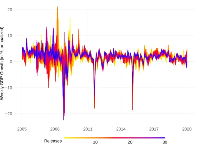
We have seen that the weekly GDP indicator is able to capture fluctuations of economic activity well ex-post. However, the real-time performance of the indicator might be dif- ferent as it is subject to revisions caused by new information from later data publications.

Figure 4 shows the indicator for its first to 30th release during the period 2005–2019.

Earlier releases (in yellow) tend to fluctuate more than later releases (in red and blue), especially during times of crisis. Further, the yellow lines are often lagging the red and

5

This analysis cannot be conducted in the same way for the Corona crisis as still not enough vintages

are available for the year 2020. We analyze the real-time performance of the indicator during this crisis

separately in the next paragraph.

blue lines. Thus, earlier releases tend to capture macroeconomic fluctuations less quickly than would be suggested by later releases. Earlier releases rely mainly on alternative and financial high-frequency series, which are the most timely available series in the data set.

Monthly series, such as business tendency surveys and retail sales, as well as realizations of quarterly GDP are included in later releases. They correct for potentially false or ex- aggerated signals from the alternative and financial data. For most periods, only a few revisions are necessary before the indicator closely approaches the stable state of later releases.

−20

−10 0 10 20

2005 2008 2011 2014 2017 2020

W eekly GDP Gro wth (in %, ann ualiz ed)

10 20 30

Releases

Figure 4: Revisions of the Weekly GDP Indicator. The figure compares the weekly GDP indicator for different releases in real time. The color bar goes from the first release in yellow over the 15th release in red to the 30th release in blue. The sample ranges from 2005 to 2019.

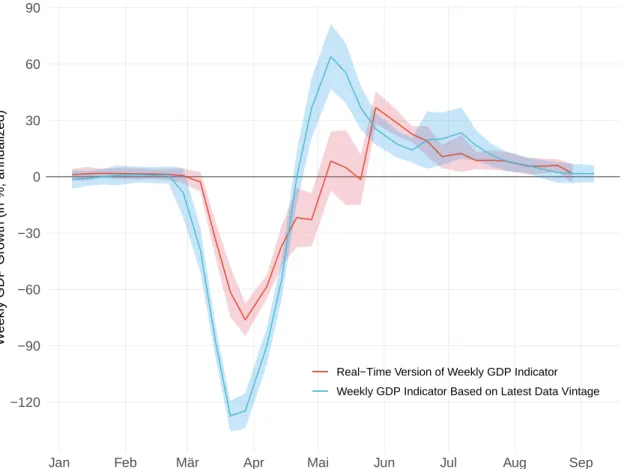
We now take a closer look on the real-time behavior of the weekly GDP indicator during the Corona crisis. Figure 5 compares the indicator as given by the last available data vintage with the real-time version of the indicator (i.e. always the first indicator release).

Again, the real-time version of the indicator can only rely on alternative and financial high-frequency data for its week-on-week assessment of GDP growth, as other variables are published with a delay and/or only for entire months or quarters. The figure reveals that the indicator has generally tracked the Corona crisis quite well in real time. Still,

6

The last available data vintage for this analysis includes all data available until November 27, 2020. This

will be updated in a later paper version.

the start of the strong downturn was captured in early March instead of in late February as suggested by the indicator in its last available version based on data which have been published at a later stage. Further, the real-time version of the indicator shows a slower recovery in April and May as compared to the latest vintage version of the indicator. Also, the size of both the trough in March and the rebound in May is initially underestimated.

Note, however, that the annualization of the weekly GDP growth rates leads to a strong visual exaggeration of this underestimation.

−120

−90

−60

−30 0 30 60 90

Jan Feb Mär Apr Mai Jun Jul Aug Sep

W eekly GDP Gro wth (in %, ann ualiz ed)

Real−Time Version of Weekly GDP Indicator Weekly GDP Indicator Based on Latest Data Vintage

Figure 5: Real-Time Version of the Weekly GDP Indicator During the Corona Crisis.

The figure compares the weekly GDP indicator as recorded by its first release (“real-time release”) with the indicator as given by the last available data vintage (currently November 27, 2020). Both indicator versions are displayed with 95%-confidence intervals.

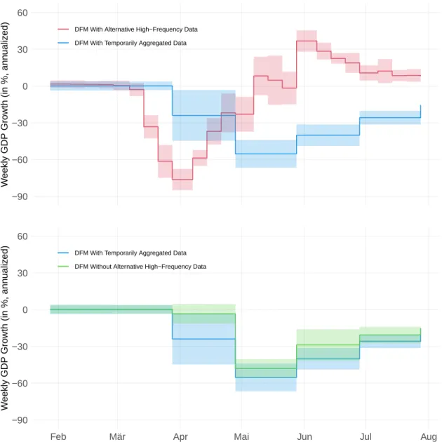
To further assess the importance of the alternative high-frequency data for capturing both the turning points as well as the extent of the Corona crisis, we compare the real-time version of the GDP indicator for three different data sets. The upper panel of Figure 6 shows the weekly GDP indicator including all data as previously (red line) in comparison with the indicator including all data, but with the alternative high-frequency data aggre- gated to monthly frequency (blue line).

The indicator using the data in weekly frequency registers the crisis much earlier. It also indicates a deeper crisis than the indicator with

7

In order to ease comparison between the weekly updated indicator and the monthly updated indicator,

both indicators are displayed by stepwise lines.

the monthly aggregated data. Further, it has smaller confidence intervals which implies that the more timely availability of the alternative data reduces the nowcast uncertainty.

−90

−60

−30 0 30 60

W eekly GDP Gro wth (in %, ann ualiz ed)

DFM With Temporarily Aggregated Data

−90

−60

−30 0 30 60

Feb Mär Apr Mai Jun Jul Aug

W eekly GDP Gro wth (in %, ann ualiz ed)

DFM Without Alternative High−Frequency Data

Figure 6: Real-Time Version of the GDP indicator for Different Data Sets. The figure shows the real-time version of the weekly GDP indicator based on three alternative data sets: the full data set including the alternative high-frequency data, the full data set but with the alternative high-frequency data aggregated to monthly frequency, and a data set where the alternative high- frequency data are excluded altogether. All indicator versions are displayed with 95%-confidence intervals.

The temporarily aggregated alternative data are available at the beginning of the follow-

ing month together with most of the macroeconomic data in our sample. Therefore, the

data are lagging the actual fluctuations of economic activity, but they might still contain

valuable additional information. To inquire this, the lower panel of Figure 6 compares the

indicator version including the temporarily aggregated alternative data (in blue) with a

GDP indicator version where no alternative high-frequency data are included at all (in

green). While both indicator versions register the crisis at the end of March, the indicator with the temporally aggregated alternative data reacts much stronger than the indicator without the alternative data. Hence, the alternative high-frequency data contain useful information beyond their timeliness. Also, the confidence interval around the indicator with the temporally aggregated alternative data is smaller than the one around the in- dicator without the alternative data. This implies that the presence of the alternative data results in a decrease in nowcast uncertainty, even if they are available at a monthly frequency only. Overall, the findings suggest that the alternative high-frequency data are very helpful for capturing the economic fluctuations during the Corona crisis.

3.3 Nowcast Exercise

This section studies the usefulness of our mixed-frequency DFM by means of a pseudo real-time out-of-sample nowcast exercise for the quarter-on-quarter growth rate of real GDP. The nowcast evaluation runs from 2005Q1 to 2020Q2 and is split into crisis periods and non-crisis periods, as discussed in Section 3.1.

The nowcast performance of the mixed-frequency DFM is evaluated for different horizons.

Specifically, we nowcast GDP growth of any quarter in the evaluation period from 12 weeks before its release (= “12-week nowcast horizon”) up to and including the last week before its release (= “1-week nowcast horizon”). This allows us to track closely how forecast errors evolve as new data get released over time.

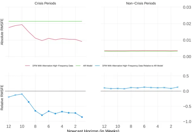
Figure 7 shows, for each of the 12 nowcast horizons, the root mean squared forecast errors (RMSFEs) of the DFM, using the full data set listed in Table 2, against an au- toregressive (AR) model of order one with intercept.

The relative RMSFE for horizon h in the lower panel of the figure is defined as ln(RMSFE

) − ln(RMSFE

), where RMSFE

(RMSFE

) is the RMSFE resulting from the DFM (AR model) nowcasts for h = 1, . . . , 12.

Unsurprisingly, the RMSFEs of both the DFM and the AR model turn out to be substantially higher for the crisis periods than for the non-crisis periods; the strong cyclical downturns and rebounds included in the crisis periods are difficult to nowcast.

The important insight is that during crisis periods, the DFM outperforms the AR model over all nowcast horizons in terms of RMSFE. The relative RMSFE improvement over the AR model increases from around 20 percent for the 12-week horizon (relative RMSFE of -0.2) to around 85 percent for the 1-week horizon (relative RMSFE of -0.85). We test for equal predictive accuracy using the test proposed by Diebold and Mariano (1995) and Giacomini and White (2006, ch. 3.4) in its one-sided version with a 10%-significance level.

8

A simple autoregressive model has been a common benchmark in previous studies. Note that the RMSFE of the AR model does not change over the nowcast horizons, since quarterly GDP is released every 12 weeks and, hence, the first lag of GDP is available for the 12-week nowcast horizon.

9

We show the log-difference of the two RMSFEs instead of their ratio, as the former is invariant to which

of the two RMSFEs is used as the basis.

Significantly greater predictive accuracy of the forecasts stemming from the DFM is in- dicated by dots in the lower panels of the figure, whereas insignificance is indicated by crosses. As can be seen from the lower left panel, during crisis periods the DFM sig- nificantly outperforms the AR model in terms of predictive accuracy for most nowcast horizons. In contrast, during non-crisis periods both models perform rather equally.

Crisis Periods Non−Crisis Periods

Absolute RMSFERelative RMSFE

12 10 8 6 4 2 12 10 8 6 4 2

0.00 0.01 0.02 0.03

−1.0

−0.5 0.0 0.5

Nowcast Horizon (in Weeks)

DFM With Alternative High−Frequency Data AR Model DFM With Alternative High−Frequency Data Relative to AR Model

Figure 7: DFM With Alternative High-Frequency Data Against AR Model. The figure shows the RMSFEs from nowcasting quarter-on-quarter real GDP growth in a pseudo real-time out-of-sample exercise. The nowcast horizon ranges from 12 weeks before GDP release up to and including the last week before release. The evaluation spans 2005Q1–2020Q2. The crisis periods include the Great Recession, the European sovereign debt crisis, the Swiss franc shock, and the Corona crisis. The dots in the lower panels indicate differences in nowcast performance that are statistically significant at a 10%-level, according to a one-sided Diebold and Mariano (1995) test.

Crosses indicate statistically insignificant differences.

A main methodological contribution of this paper is to provide a mixed-frequency DFM which can easily account for serial correlation in the errors of the factor measurement equation, despite several mixed frequencies, missing observations, ragged edges and data histories of different lengths (see Section 2.2). It turns out that this feature is indeed important for achieving a good nowcast performance in our application. This is discussed in Appendix A.8.

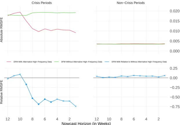
The DFM presented in Figure 7 uses the full data set, which includes the alternative high-

frequency data as well as the standard financial and macroeconomic series. We want to

know whether the use of the alternative high-frequency data, in addition to the standard

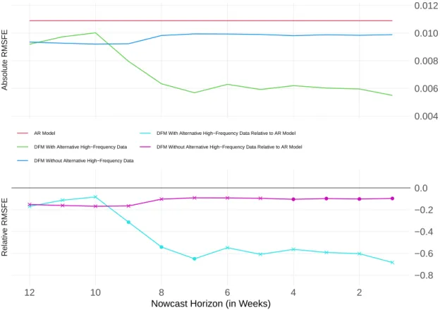
variables, actually helps to improve the nowcast performance. For this purpose, Figure 8 depicts the RMSFEs of the DFM including the full data set against the RMSFEs of the DFM, excluding the alternative high-frequency series. The DFM using the full data set clearly outperforms the DFM without the alternative high-frequency data, although only in crisis periods as can be seen from the lower left panel of the figure. Note that, for the 4- to 1-week nowcast horizons, the nowcast error difference between the two specifications is close to the chosen significance threshold with p-values being between 11 and 12 percent.

Crisis Periods Non−Crisis Periods

Absolute RMSFERelative RMSFE

12 10 8 6 4 2 12 10 8 6 4 2

0.000 0.005 0.010 0.015 0.020

−0.75

−0.50

−0.25 0.00 0.25

Nowcast Horizon (in Weeks)

DFM With Alternative High−Frequency Data DFM Without Alternative High−Frequency Data DFM With Relative to Without Alternative High−Frequency Data

Figure 8: DFM With and Without Alternative High-Frequency Data. Notes: See Figure 7.

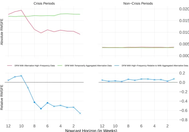
Further, we are interested in knowing whether the value of the alternative data for now-

casting GDP comes from its timeliness, or whether the data are even valuable if they are

sampled at a monthly frequency only. Figure 9 shows the RMSFEs of the DFM including

the full data set against the RMSFEs of the DFM including the full data, but with all

data aggregated to the monthly frequency. These temporarily aggregated observations are

available in the first week of the next month (together with, for instance, the monthly busi-

ness tendency surveys). The lower left panel reveals that the higher frequency increases

the nowcast performance for crisis periods. Note that, for the 5- to 1-week nowcast hori-

zons, the difference between the two specifications is again close to the chosen significance

threshold with p-values being between 11 and 13 percent.

Crisis Periods Non−Crisis Periods

Absolute RMSFERelative RMSFE

12 10 8 6 4 2 12 10 8 6 4 2

0.000 0.005 0.010 0.015 0.020

−0.8

−0.6

−0.4

−0.2 0.0 0.2

Nowcast Horizon (in Weeks)

DFM With Alternative High−Frequency Data DFM With Temporarily Aggregated Alternative Data DFM With High−Frequency Relative to With Aggregated Alternative Data

Figure 9: DFM With and Without Temporal Aggregation. Notes: See Figure 7.

In a further step, we compare the nowcast accuracy by joining the crisis and non-crisis periods to one single evaluation phase from 2005Q1 to 2020Q2. As can be seen from the blue line in the lower panel of Figure 10, the DFM including the full data set outperforms the AR model in terms of RMSFE for all horizons. The difference in the nowcast per- formance is statistically significant for the 9- to 7-week horizons and at least close to the chosen significance level for the 6- to 1-week horizons (p-values at 11 percent). The DFM excluding the alternative high-frequency data also outperforms the AR model (see pink line in the lower panel), although to a much smaller extent as the full data DFM. The same holds true for the DFM with the data aggregated to the monthly frequency (not shown in the figure). It is noteworthy that the differences in nowcast performance during the crisis periods almost entirely drive the RMSFE results for the joint evaluation phase, although the crisis periods account only for 12 quarters of the total 79 quarters during 2005Q1 to 2020Q2.

In order to verify the robustness of the results, Appendix A.7 presents Figures 7 to 10

with mean absolute percentage errors (MAPEs) instead of RMSFEs. The MAPE results

turn out to be similar to the RMSFE results and all conclusions remain unchanged.

Absolute RMSFERelative RMSFE

12 10 8 6 4 2

0.004 0.006 0.008 0.010 0.012

−0.8

−0.6

−0.4

−0.2 0.0

Nowcast Horizon (in Weeks)

AR Model

DFM With Alternative High−Frequency Data DFM Without Alternative High−Frequency Data

DFM With Alternative High−Frequency Data Relative to AR Model DFM Without Alternative High−Frequency Data Relative to AR Model

Figure 10: Joint Evaluation for Crisis and Non-Crisis Periods. Notes: See Figure 7.

4 Conclusion

In this paper, we propose a novel dynamic factor model for high- and mixed-frequency

data with stochastic volatility and serial correlation in the measurement errors. The model

consists of three interdependent state-space blocks: data augmentation, dynamic factor

and stochastic volatility, where the former block is novel in the DFM literature. Previous

mixed-frequency DFMs have disregarded unobserved information in the mixed-frequency

data and have estimated a dynamic factor conditional on observed data only, typically

using a modified Kalman filter. In contrast, we propose to estimate all unobserved in-

formation conditional on observed data in the data augmentation block and to estimate

the dynamic factor conditional on the observed as well as the estimated latent data in

the dynamic factor block. Importantly, the augmentation from sparse observed data to a

balanced panel with observed and latent data information allows us to quasi-difference the

measurement equation of the dynamic factor. Thereby, our DFM can easily account for

serial correlation in the factor measurement errors despite mixed frequencies, publication

lags, data histories of different lengths and missing observations in the data. This allows

the common factor to have less explanatory power for the mixed-frequency series over

a longer period of time while having high explanatory power during other periods. In

contrast to previous literature, we take a fully Bayesian approach to estimate the model,

where the joint posterior distribution is simulated with Gibbs sampling. A further con-

tribution of the paper is that we extend the sampling procedure of Chan and Jeliazkov

(2009) to the case of mixed-frequency data and use it for the estimation of the latent data, the dynamic factor and the stochastic volatility. This extension is done by integrating the temporal aggregation scheme originally proposed by Mariano and Murasawa (2003) into the sampler.

As an empirical application, we construct a weekly GDP indicator using a broad set of daily, weekly, monthly and quarterly series. The set includes a variety of so-called alter- native high-frequency data, such as daily credit card transactions, smartphone mobility tracking, and Google trends search queries. Our model is well suited to extract the busi- ness cycle information in these data. We look especially at four periods of sudden and strong economic fluctuations, namely the Great Recession, the European sovereign debt crisis, the Swiss franc shock and the Corona crisis. It turns that the weekly indicator tracks economic activity nicely during the aforementioned periods. The economy went down and up again so quickly during these periods that looking at monthly or quarterly figures only does not reveal the full dimension of the fluctuations. A special finding for the Corona crisis is that GDP growth fell deeply into negative territory already before the government imposed a lockdown, as consumers and producers reduced their activities in light of the pandemic. This qualifies the relevance of the lockdown for the negative economic consequences of the crisis. We take a further look at the Corona crisis and study the real-time behavior of the weekly GDP indicator during this period. Although the indicator is generally subject to revisions as more and more data become available over time, it captures the sudden and steep economic downturn and the nearly equally steep rebound during the the year 2020 quite timely and accurately in real time. We find that this is mainly due to the inclusion of the alternative high-frequency data. Our analysis further yields that even when using these data in monthly intervals only, their inclusion would still have helped to register the downturn more timely than when just using stan- dard data. However, the main benefit comes from using the data at a high frequency.

We complement the empirical application with a pseudo real-time out-of-sample now- cast exercise for quarterly GDP from 2005Q1 to 2020Q2. It turns out that our mixed- frequency DFM significantly outperforms an AR benchmark model during crisis periods.

The RMSFE decreases by between 20 and 85 percent for horizons from 12 weeks to one

week before GDP release. Even when including the alternative data in monthly intervals

only, they help to improve the forecast accuracy. In contrast, we find no significant im-

provements for non-crisis periods. We conclude that alternative high-frequency data can

be very helpful when the economy moves strongly and suddenly, but they just add noise

during stable times. On a last note, the differences in nowcast performance during the

crisis periods turn out to be so big that they dominate the results for a joint evaluation of

crisis and non-crisis periods. This is despite the fact that the crisis quarters only account

for 15 percent of all quarters in the evaluation phase. The ultimate lesson here is: when

constructing new nowcast models, it is of utmost importance to focus on a good perfor-

mance for major economic downturns and upturns, while normal economic times can be handled equally well with existing simple models.

References

Aruoba, S. B., Diebold, F. X., and Scotti, C. (2009). Real-Time Measurement of Business Conditions. Journal of Business & Economic Statistics, 27(4):417–427.

Aßmann, C., Boysen-Hogrefe, J., and Pape, M. (2016). Bayesian Analysis of Static and Dynamic Factor Models: An Ex-Post Approach Towards the Rotation Problem. Journal of Econometrics, 192(1):190–206.

Bai, J. and Wang, P. (2015). Identification and Bayesian Estimation of Dynamic Factor Models. Journal of Business & Economic Statistics, 33(2):221–240.

Bańbura, M., Giannone, D., and Reichlin, L. (2011). Nowcasting. In Clements, M. P.

and Hendry, D. F., editors, The Oxford Handbook on Economic Forecasting, chapter 2, pages 193–224. Oxford University Press, Oxford.

Bańbura, M. and Modugno, M. (2014). Maximum Likelihood Estimation of Factor Models on Datasets with Arbitrary Pattern of Missing Data. Journal of Applied Econometrics, 29(1):133–160.

Camacho, M. and Perez-Quiros, G. (2010). Introducing the Euro-Sting: Short-Term In- dicator of Euro Area Growth. Journal of Applied Econometrics, 25(4):663–694.

Carter, C. K. and Kohn, R. (1994). On Gibbs Sampling for State Space Models.

Biometrika, 81(3):541–553.

Chan, J., Leon-Gonzalez, R., and Strachan, R. W. (2018). Invariant Inference and Ef- ficient Computation in the Static Factor Model. Journal of the American Statistical Association, 113(522):819–828.

Chan, J. C. and Jeliazkov, I. (2009). Efficient Simulation and Integrated Likelihood Es- timation in State Space Models. International Journal of Mathematical Modelling and Numerical Optimisation, 1(1-2):101–120.

Chib, S. and Greenberg, E. (1994). Bayes Inference in Regression Models With ARMA (p, q) Errors. Journal of Econometrics, 64(1-2):183–206.

Diebold, F. X. and Mariano, R. S. (1995). Comparing Predictive Accuracy. Journal of Business & Economic Statistics, 13(3):253–263.

Doz, C., Giannone, D., and Reichlin, L. (2011). A Two-Step Estimator for Large Approx-

imate Dynamic Factor Models Based on Kalman Filtering. Journal of Econometrics,

164(1):188–205.

Eckert, F. and Mikosch, H. (2020). Mobility and Sales Activity During the Corona Crisis:

Daily Indicators for Switzerland. Swiss Journal of Economics and Statistics, 156(1):1–

10.

Eraslan, S. and Götz, T. (2020). An Unconventional Weekly Economic Activity Index for Germany. Deutsche Bundesbank Technical Paper.

Frühwirth-Schnatter, S. (1994). Data Augmentation and Dynamic Linear Models. Journal of Time Series Analysis, 15(2):183–202.

Giacomini, R. and White, H. (2006). Tests of Conditional Predictive Ability. Economet- rica, 74(6):1545–1578.

Giannone, D., Reichlin, L., and Small, D. (2008). Nowcasting: The Real-Time Informa- tional Content of Macroeconomic Data. Journal of Monetary Economics, 55(4):665–676.

Guggia, V., Indergand, R., and Wegmüller, P. (2020). Neuer Index zur Wöchentlichen Wirtschaftsaktivität (WWA). Konjunkturtendenzen SECO Winter 2020/21.

Kim, C.-J. and Nelson, C. R. (2017). State-Space Models with Regime Switching: Classical and Gibbs-Sampling Approaches with Applications. The MIT Press.

Kim, S., Shepherd, N., and Chib, S. (1998). Stochastic Volatility: Likelihood Inference and Comparison With ARCH Models. Review of Economic Studies, 65(3):361–393.

Lewis, D. J., Mertens, K., Stock, J. H., and Trivedi, M. (2020). Measuring Real Activity Using a Weekly Economic Index. Federal Reserve Bank of New York, 920.

Marcellino, M., Porqueddu, M., and Venditti, F. (2016). Short-Term GDP Forecasting With a Mixed-Frequency Dynamic Factor Model With Stochastic Volatility. Journal of Business & Economic Statistics, 34(1):118–127.

Mariano, R. S. and Murasawa, Y. (2003). A New Coincident Index of Business Cycles Based on Monthly and Quarterly Series. Journal of Applied Econometrics, 18(4):427–

443.

Primiceri, G. E. (2005). Time Varying Structural Vector Autoregressions and Monetary Policy. The Review of Economic Studies, 72(3):821–852.

Stock, J. H. and Watson, M. W. (2002). Macroeconomic Forecasting Using Diffusion Indexes. Journal of Business & Economic Statistics, 20(2):147–162.

Tanner, M. A. and Wong, W. H. (1987). The Calculation of Posterior Distributions by Data Augmentation. Journal of the American Statistical Association, 82(398):528–540.

Wallis, K. F. (1986). Forecasting With an Econometric Model: The ‘Ragged Edge’ Prob-

lem. Journal of Forecasting, 5(1):1–13.

A Appendix

A.1 Temporal Aggregation

Temporal aggregation of the high frequency factor f

to any lower frequency factor f

is straightforward for stock variables such as interest rates or business tendency surveys. In these cases, temporal aggregation is simply given by an average:

f

=

k−1

X

i=0

λ

f

, where λ

=

and where k denotes how many times the high frequency occurs within the low frequency (e.g., k = 3 for aggregation of monthly to quarterly data). The case of flow variables, such as GDP or retail sales, is slightly more complicated. Since these variables typically enter forecasting models in growth rates, any temporal aggregation involves nonlinearities.

An approximation based on geometric instead of arithmetic means has been proposed by Mariano and Murasawa (2003) and has since been widely adopted (see, e.g., Bańbura et al., 2011, and Marcellino et al., 2016):

f

=

s

X

i=0

λ

f

, where λ

=

and where the number of distributed lags is given by s = 2(k − 1). The geometric mean based aggregation implies a triangular weighting scheme that accounts for the statisti- cal overhang occuring during the aggregation of growth rates. This is illustrated in the following: Let X be a flow variable and let

log X

= 1

3 (log X

+ log X

+ log X

).

Growth in the second quarter is then given by logX

− log X

=

1

3 (log(X

+ log X

+ log X

) − 1

3 (log X

+ log X

+ log X

)

= 1

3 (log X

− log X

) + 1

3 (log X

− log X

) + 1

3 (log X

− log X

).

Next, introduce additional terms into the equation:

logX

− log X

= 1

3 (log X

− log X

+ log X

− log X

+ log X

− log X

)+

1

3 (log X

− log X

+ log X

− log X

+ log X

− log X

)+

1

3 (log X

− log X

+ log X

− log X

+ log X

− log X

).