Earnings Differences between Chinese andIndian Wage Earners, 1987–2004

Earnings Differences between Chinese and Indian Wage Earners, 1987–2004

Olivier Bargain

Sumon Kumar Bhaumik Manisha Chakrabarty Zhong Zhao

DISCUSSION PAPER SERIES

Forschungsinstitut zur Zukunft der Arbeit Institute for the Study of Labor

January 2008

Earnings Differences between Chinese and Indian Wage Earners, 1987–2004

Olivier Bargain

University College Dublin, CHILD and IZA

Sumon Kumar Bhaumik

Brunel University, WDI and IZA

Manisha Chakrabarty

Indian Institute of Management

Zhong Zhao

IZA

Discussion Paper No. 3284 January 2008

IZA P.O. Box 7240

53072 Bonn Germany

Phone: +49-228-3894-0 Fax: +49-228-3894-180

E-mail: iza@iza.org

Any opinions expressed here are those of the author(s) and not those of IZA. Research published in this series may include views on policy, but the institute itself takes no institutional policy positions.

The Institute for the Study of Labor (IZA) in Bonn is a local and virtual international research center and a place of communication between science, politics and business. IZA is an independent nonprofit organization supported by Deutsche Post World Net. The center is associated with the University of Bonn and offers a stimulating research environment through its international network, workshops and conferences, data service, project support, research visits and doctoral program. IZA engages in (i) original and internationally competitive research in all fields of labor economics, (ii) development of policy concepts, and (iii) dissemination of research results and concepts to the interested public.

IZA Discussion Papers often represent preliminary work and are circulated to encourage discussion.

Citation of such a paper should account for its provisional character. A revised version may be available directly from the author.

January 2008

ABSTRACT

Earnings Differences between Chinese and Indian Wage Earners, 1987-2004

This paper is one of the first comprehensive attempts to compare earnings in urban China and India over the recent period. While both economies have grown considerably, we illustrate significant cross-country differences in wage growth since the late 1980s. For this purpose, we make use of comparable datasets, estimate Mincer equations and perform Oaxaca-Blinder decompositions at the mean and quantile decompositions at different points of the wage distribution. The initial wage differential in favour of Indian workers, observed in the middle and upper part of the distribution, partly disappears over time. While the 1980s Indian premium is mainly due to higher returns to education and experience, a combination of price and endowment effects explains why Chinese wages have caught up, especially since the mid-1990s. The price effect is only partly explained by the observed convergence in returns to education; the endowment effect is driven by faster increase in education levels in China and significantly accentuates the reversal of the wage gap in favour of this country for the first half of the wage distribution.

JEL Classification: O15, J24, O53, P52

Keywords: China, India, earnings, returns to education, quantile regression, Oaxaca-Blinder decomposition

Corresponding author:

Olivier Bargain

Departments of Economics University College Dublin Belfield, Dublin 4

Ireland

E-mail: olivier.bargain@ucd.ie

* The authors have benefited from conversations with Gary Fields, Richard Freeman, Jim Albrecht and with participants to the IARIW-NBS conference (Beijing, September 2007). They remain grateful to Blaise Melly for the Stata code on the QR decomposition algorithm, and to the IZA and the CHIPS project for providing the Indian and Chinese data, respectively. Bargain and Bhaumik would like to

1. Introduction

A growing literature compares average earnings or wage distributions across countries and investigates how standard human capital factors can explain these wage differentials, relying in particular on the well-known Oaxaca-Blinder decomposition or some of its extensions. For instance, Blau and Khan (1996) compare the distributions of male wages across ten industrial countries and study to which extent differences are explained by returns to education.

Bourguignon et al. (2007) extend the Oaxaca-Blinder technique to decompose differences in household income distributions, and therefore household inequality measures, between the US and Brazil. Almeida dos Reis and Paes de Barros (1991) study changing wage distributions across regions in Brazil. Donald et al. (2000) simulate counterfactual density functions to decompose differences in wage distributions between the USA and Canada.

It is tempting to compare India and China along these lines. With respectively 1.3 and 1.1 billion inhabitants, these countries represent the largest pool of workers in the world. India and China have also experienced a similar timing of economic take-off,¹ and have both expanded by 50% in real terms over the 1990s thanks to market-oriented reforms. Their similarities make them natural comparators. While many aspects of their rapid growth have been explored in the literature, it seems equally important to understand how growth has affected wage progression and how these countries compare in this respect. Wage determinants have been analysed for each countries separately, including numerous estimations of returns to education for various time periods. ² Yet, no systematic attempt has been made to compare wage distributions in India and China as well as their determinants.

Focusing on the urban sector in both countries, this paper attempts to provide a comprehensive description of Indo-Chinese wage differentials since the late 1980s. We address the cross-country comparison by gathering earnings data with comparable variable definitions across countries and for comparable periods. We also make use of the standard Mincer equation to perform Oaxaca-Blinder decompositions of the mean wage difference as well as recently developed quantile decompositions. This way, we examine the extent to which Indo-Chinese wage differences can be explained by differences in workers’

characteristics (experience, education, etc.) and returns to these characteristics, both on average and for the whole wage distribution.³

We find that the Indo-Chinese wage gap, which was in favour of Indian wage earners in the late-1980s, has declined over time. In the late 1980s and first half of the 1990s, there is no systematic difference in composition between Indian and Chinese wage earners, and the wage gap is mainly explained by a price effect driven by much higher returns to education in India.

Over this period, however, returns to characteristics start to decrease in the upper earnings quantiles. In the late 1990s/early 2000s, a rapid increase in Chinese earnings leads to a reversal of the wage gap for most of the distribution. This is due to a combination of price and endowment effects. The price effect is only partly on account of rapidly increasing

1 Both countries have experienced a development strategy relying on manufacturing industry in the 1950s/60s, deregulation in the 1980s and restructuration of the economies towards more balanced strategies in the recent years.

2 Papers in which returns to education were estimated include Byron and Manaloto (1990), Liu (1998), Knight and Song (2003), Zhang et al. (2005) and Appleton et al. (2005) for China, and Saha and Sarkar (1999), Kingdon and Unni (2001), Duraisamy (2002) and Kijima (2006) for India.

3 Note that we do not address the question of income inequality since this would require considering household income rather than individual wages. The extension of the decomposition approach to household income distributions involves at least two additional dimensions (other than observed characteristics and returns to these characteristics), namely occupational status of household members and household composition. Bourguignon et al. (2007) suggest one of the first regression-based approaches in this direction.

returns to education in China. Interestingly, a faster improvement in the average educational endowments of the Chinese wage earners also contributes to the reversal of the wage gap in the first half of the earnings distribution. Overall, it seems that the more profound changes that have occurred in China over the past 25 years drive the bulk of the evolution in the Indo- Chinese wage differential.

The rest of the paper is structured as follows. In section 2, we report the nature of the data, the associated descriptive statistics and first international comparisons of wage distributions.

Earnings estimations, and returns to education and to experience in particular, are presented and discussed briefly in section 3. Sections 4 and 5 report the results of the decomposition analysis, respectively at the mean and for the entire distribution. Section 6 concludes.

2. Data Description and Wage Differential

Our empirical exercise is based on earnings data for regular wage earners in India and China.

The data on the Indian wage earners are obtained from the 1987, 1993 and 2004 rounds of the National Sample Survey (NSS). These pan-Indian surveys are organised by the Central Statistical Organisation, and they use a stratified random sampling scheme to collect the data.

The stratification is along geographical lines, with each state, as well as each district within a state, getting adequate representation (see Kijima, 2006). The Employment and Unemployment Schedule of the NSS is the only source of information for earnings and worker characteristics in India. It is stylised to exclude from the sample self-employed and casual workers, such that the sample only includes wage earners who work full time and do not attend school. In addition, possibly to minimise measurement error, it is customary to restrict the sample to urban workers who account for 85% of all wage earners in the sample (see Kijima, 2006).

The Chinese data are obtained from the 1988, 1995 and 2002 waves of the China Household Income Project (CHIP).⁴ Based on the large sample used by the National Bureau of Statistics, each of the three surveys gathers information from over 20,000 individuals, covering both rural and urban regions in eleven provinces in China and resembling the actual distribution of populations across these regions (see Demurger et al., 2006).⁵ In order to make the Chinese sample comparable with the Indian sample, we restrict the former to urban wage earners working full time, thereby making the sample similar to the one used by Liu (1998), Knight and Song (2003) and Zhang et al. (2005).

Both surveys provide information on earnings, age, education and gender of labour force participants, plus industry types and country-specific variables. We further restrict both samples to 21-60 year olds. In order to make the earnings data comparable across the countries and the years, we transform all (weekly) wages into 2000 PPP USD equivalent, using the World Development Indicators on consumer price indices and PPP conversion factors.⁶ Finally, we harmonise education variables. While the NSS/Indian survey and 1988 wave of the CHIP/Chinese data include information on the levels of education alone, the

4 The CHIP project was jointly set up in 1987 by the Institute of Economics of the Chinese Academy of Social Sciences, the Asian Development Bank and the Ford Foundation; it also received support from the East Asian Institute of Columbia University.

5 Provinces are Beijing, Shanxi, Liaoning, Jiangsu, Anhui, Henan, Hubei, Guangdong, Sichuan, Yunnan and Gansu. The 1988 data covers 10 provinces. In 1995, Sichuan province was added in the survey. In 2000, Chongqing was separately from Sichuan and became a provincial-level city itself but is here treated as part of Sichuan. Note that Zhang et al. (2005) use data on Beijing, Shanxi, Liaoning, Zhejiang, Guangdong, Sichuan, and argue that these six provinces are broadly representative of China’s rich regional variation.

6 Limitations to this adjustment are discussed in the concluding section. Details about the construction of PPP- adjusted earnings measures and the comparable educational variables are available upon request to the authors.

1995 and 2002 waves of CHIP data include both the number of schooling years and education levels. Then, we construct four education categories – no education or primary education, middle secondary education, high secondary education, and college education – that are comparable across countries and periods.⁷ Hereafter, period 1 refers to year 1987 for India and 1988 for China, period 2 to 1993 and 1995 respectively, period 3 to 2004 and 2002.

This is not a perfect time comparison but the best that could be done with available data.⁸ Descriptive statistics for the CHIP/Chinese data and the NSS/Indian data are reported in Tables 1a and 1b, for men and women respectively. They indicate that in all three periods, Chinese wage earners in our sample are older on average than their Indian counterparts, and hence have larger potential experience. Women constitute a significantly greater proportion of the wage earning work force in China – around half of the workers – than in India, perhaps reflecting higher educational attainment of an average Chinese woman;⁹ or the socialist ideology that promotes equal employment opportunity for men and women.

It is evident that while India had an educational advantage in the late 1980s, the situation has changed rapidly since 1990s. In 1987-88, i.e., period 1 of our analysis, 23% (32%) of the male (female) wage earners were college graduates in India compared to only 18% (9%) in China.¹⁰ By 2002-04, however, the picture had changed remarkably, with 39% (34%) of Chinese male (female) wage earners achieving a college degree. Moreover, while almost all of the Chinese workers had at least middle secondary education in the last period, 29% of women and 19% of men still had only primary or no education in India. The rapid skill increase in China is in line with the significant shift in the structure of this economy in the late 1990s – with high technology industries and services progressively accounting for greater share of value added and employment – and is also driven by strong political impulses.¹¹ As we shall see, higher educational endowment in China in the recent period has influenced significantly the wage differential across the two countries.

Tables 1a and 1b also report industry types, which are made comparable across countries.

Manufacturing remains the largest sector in terms of male labour force in both countries, with a declining share over time. As expected, it represents a larger proportion of the labour force in China and also employs a large share of women in this country. Services are the main employer for women in both countries, with a very large share in India and an increasing trend over time.¹² The size of public administration has become very comparable across countries in the last period.

7 The use of education categories, while somewhat unusual in the Chinese context, can be found in other studies as well (e.g., Liu, 1998). We have also translated education levels into years of education when it was missing;

for India, the exercise is complicated by the fact that there is variation across states and we follow the approach of Kijima (2006). This is used in particular to obtain a proxy measure for experience, computed as age minus schooling minus six (years prior to school enrolment).

8 We initially had a better period match using the China Health and Nutrition Survey, but sample sizes were too small.

9 Female literacy rate in China was 86% in 2002, compared with 48% in India in 2003.

10 This is in line with the fact that growth in India has relied significantly on expansion of the skill-intensive service sector (in particular business services, communication services and banking) and also skill-based manufacturing industries (like auto ancillaries and pharmaceuticals). This is in contrast with the growth path in China, and notably that of the manufacturing sector which was primarily labour-intensive and did absorb surplus agricultural labour.

11 In the recent period, it is a manifestation of a bank-financed investment of RMB 200 billion (about USD 25 billion) in universities since 1998, which supplemented the government’s budgetary support of about RMB 150 billion (USD 20 billion) for secondary and higher education (2000 figures).

12 For the whole selected sample of men and women, the service sector represents 23% of the labour force in India and 17% for China in the mid 1990s, which can be compared to the figures provided by the KILM database of the ILO (20% and 15% respectively).

Table 1a: Descriptive statistics (men)

Table 1b: Descriptive statistics (women)

Tables 1a and 1b finally report mean weekly earnings of Indian and Chinese wage earners at each period. It is easily verified that the compounded annual growth rate of average earnings between periods 1 (1987-88) and 3 (2002-04) was around 3% in India and 7% in China. At the same time, the GDP per capita for India (China) was 1569 (1528) in period 1 and 2553 (4568) in period 3, measured in 2000 PPP USD, which gives a compounded growth rate of around 3.5% (8%) on average per year. Thus the difference in wage progression between the two countries reflects to some extent differences in overall economic performance; this should appear in some of our results below.¹³

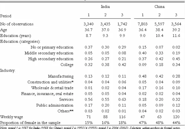
To go beyond average figures, we compute log earnings (in 2000 PPP USD) at different quantiles for each country, as depicted in the two left hand side quadrants of Figure 1. The graphs reflect the fast earnings growth in China and the very modest changes in India previously encountered. Notice that the wage progression in India benefits mostly to the second half of the distribution. In China, wage growth is larger for higher quantiles between periods 1 (1987-88) and 2 (1993-95) but is more equally shared between period 2 and 3 (2002-04). The right hand side quadrant is simply the difference of the two latter, i.e. it plots the Indo-Chinese difference in earnings. It is positive for nearly all deciles of the earnings distribution in periods 1 and 2; however, by period 3, the earnings gap had turned in favour of China for the lower half of the distribution, and was significantly reduced for the upper deciles.

Figure 1: Log-wage Distributions

China

2.50 3.00 3.50 4.00 4.50 5.00 5.50 6.00

10% 30% 50% 70% 90%

Quantiles

log wage

period 1 (1987-88) period 2 (1993-1995) period 3 (2002-2004)

India-China Gap

-0.60 -0.40 -0.20 0.00 0.20 0.40 0.60 0.80 1.00

10% 30% 50% 70% 90%

Quantiles

log wage difference

India

2.50 3.00 3.50 4.00 4.50 5.00 5.50 6.00

10% 30% 50% 70% 90%

Quantiles

log wage

3. Earnings equations

We then proceed with the estimation of standard Mincer equations using comparable data and specifications. Following the bulk of the literature, we estimate, for each country and for men and women separately, equations of the form:

ε δ

γ α

α

α ^{+ + +}

∑

∑

=

j

j j

i

i

iEDUC CONTROLS

EXP EXP

Y _{0 1 2} ²

ln (1)

13 The exercise suggested in this paper simply attempts to quantify how much of the cross-country wage differential can be explained by human capital factors as traditionally available in micro data (e.g. education, experience, etc.) and returns to these characteristics; yet, workers’ skills are only part of the economic factors explaining the productivity of labour. Fully explaining differences in productivity between countries is beyond the scope of this paper and a broader picture would attempt to reconcile micro and macro aspects. We simply refer here to Bosworth and Collins (2007) for a recent study using growth accounting to compare India and China.

where Y is (weekly) earnings, EXP is potential experience as previously defined, and EDUC is a vector of dummies capturing three different education levels (‘no or primary education’ is the omitted category). Control variables include industry types as previously described (‘public administration’ is the omitted category). Country-specific controls are also added at this stage, including regional dummies, Han ethnicity and membership of the communist party (for China); religion dummies and caste-specific public sector jobs (for India).

The Mincer equation (1) is estimated using ordinary least square (OLS). In addition, we estimate the effects of covariates on earnings at different points of the conditional distribution using quantile regression (QR) (Koenker and Bassett, 1978). Results are typically reported for three points only, namely the 25^th centile, the median and the 75^th centile. Note that we do not account, in our estimation, for selection bias, i.e., the possibility that the workers in our sample did not become wage earners randomly but on account of some individual and household characteristics.¹⁴

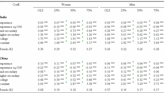
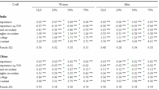
Estimates are reported in Tables A1 to A3 in the Appendix for both countries and for men and women separately. We present only results for the main variable of interests which are common determinants of earnings in both countries, including experience and education.¹⁵ Corresponding coefficients are mostly significant and R-square values indicate a reasonable degree of fit, of a comparable order to findings by Appleton et al. (2005) and Zhang et al (2005) in the case of China and Duraisamy (2002) and Kijima (2006) for India. These studies provide rich discussions about wage determinants and links to policy and historical developments in the 1980s and 1990s in both countries. Then, to avoid redundant analysis, we simply focus hereafter on returns to experience and education for the sake of the cross- country comparison over time.

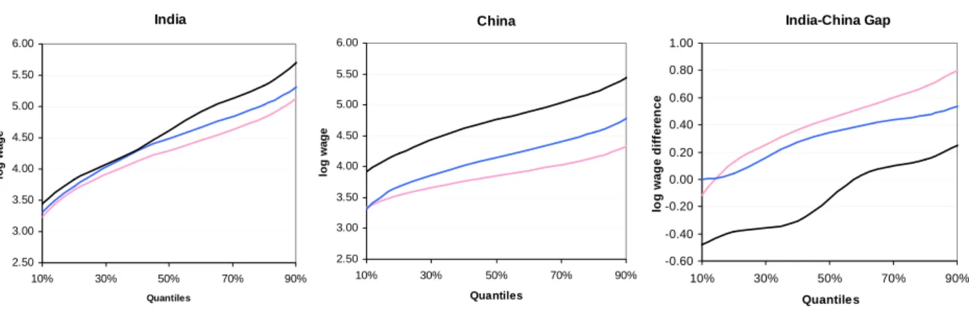
Firstly, we use OLS estimates to compute the experience-earnings profile, as plotted in Figure 3. As observed in most countries, this relation has an inverted-U shape. Important changes occur in China, with a substantial increase between late 1980s and the mid-1990s followed by a sharp decline until 2002; very similar profiles are depicted in Appleton et al.

(2005). Knight and Song (2003) argue that the rapid increase between 1988 and 1995 may have been on account of the more experienced workers appropriating a greater than proportionate share of the (ostensibly performance-based) bonuses that were legitimised in the 1980s. Over-rewarding seniority seems to be a central feature of the pre-reform wage structure, resulting in higher returns to experience than in several industrialised countries like the UK, the US or Australia in the 1980s and 1990s (Meng and Kidd, 1997). Appleton et al.

(2005) argue that the strong correction that occurred after 1995 was due to the fact that senior workers were the most at risk from retrenchment by enterprises attempting to increase profitability and by the government’s initiative to reform and restructure state-owned enterprises.¹⁶ Figure 3 indicates that return to experience was higher, on average, in India than in China, except in period 2 and for women with up to 30 years of experience. Returns to experience seem fairly constant in India over time and the cross-country difference in returns between the two countries is, as a result, essentially driven by the aforementioned trend in

14 Individual workers in developing countries with surplus labour often do not have the ability to choose between forms of employment; choice of sectors and types of occupation is often accidental and driven by patterns of labour demand (Fields, 2005). Note also that introducing selection in QR decomposition is as yet not common practice (among a few exceptions, see Albrecht et al., 2006, who account for female participation decisions).

15 Complete results are available upon request to the authors.

16 As explained by Knight and Song (2003), the fact that the profile peaked earlier in 1995 and fell dramatically for older workers is consistent with a move to a more productivity-based and a less bureaucratically-based earnings structure. The authors also extensively discuss changes in labour market policy and economic structure in China during the 1980s and 1990s and their impact on wage settlements.

Chinese returns. In particular, the adjustment occurring in China between periods 2 and 3 is expected to appear in our decomposition results and play in favour of Indian wages.

Figure 2: Wage Progression

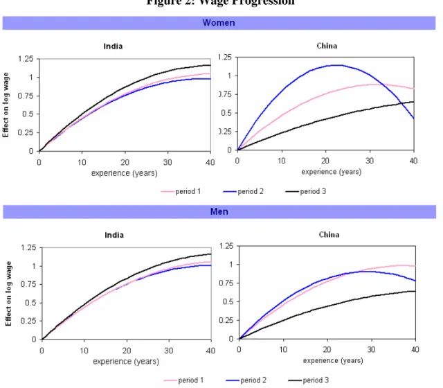
Next, we focus on returns to education obtained using both OLS and QR estimations. Results are qualitatively consistent with earlier estimates for both countries (see footnote 2).¹⁷ In Tables A1 to A3 in the Appendix, QR estimates indicate that returns increase consistently with the education level, for both countries, for all time periods, and for all earnings quantiles.

Significant differences between China and India appear in the levels of returns to education and their evolution over time. To make it clear, we plot in Figure 4 the cross-country net difference in returns at each period, for the mean, 25^th centile, median and 75^th centile.

Returns to education are higher in India at all periods and for both men and women, particularly for higher secondary and college education.¹⁸ Estimates of Tables A1 to A3 show that returns seem to rise very slowly in India between periods 1 and 2 and even decrease slightly for secondary education between periods 2 and 3. At the same time, returns in China rose by and large, especially for college education and, to a lesser extent, higher secondary

17 Estimates reported in Tables A1 to A3 are not directly comparable to those of studies using years of schooling as opposed to discrete educational categories (for instance Zhang et al., 2005, for China). However, results are broadly reconciled if we use an alternative specification using schooling years.

18 These very high returns are partly on account of the rent people with higher education can charge and partly on account of the pattern of industrialisation specific to India, that is, service sector and skill intensive sector driven, as opposed to mass manufacturing driven.

education.¹⁹ Men’s returns increased gradually over the whole period under study while women’s returns rose especially between periods 2 and 3. These trends result in the differences highlighted in Figure 4, showing that returns to education in China partly catch up over the whole period, with a gradual catch up for men. In the case of women, the Indian advantage almost stagnates between period 1 and 2 – it increases very slightly on average and for the first half of the wage distribution – but decreases significantly between the mid-1990 and the early 2000s. For both men and women alike, the catching up in Chinese returns to education is especially fast for lower quantiles, which, according to estimates of Tables A1 and A3, is due to increase in Chinese returns but also to decrease in Indian returns at the 25^th centile. We can anticipate that in the QR decomposition exercise (cf. section 5), this trend shall contribute to improve the relative situation of Chinese wage earners, especially in the lower part of the distribution.

Figure 3: Indo-Chinese Difference in Returns to Education

19 These results are consistent with increased demand for skilled labour (in particular due to skill-biased technological change) and with the hypothesis of an increasingly competitive labour market, in connection to the stated policy of the Chinese government to closely link productivity and earnings of wage earners since the 1980s (see Liu, 1998; Mauer-Fazio, 1999; Knight and Song, 2003); other aspects may have come into play, including the liberalization of controls on migration that increased the supply of low-skill labour in urban areas (see Appleton et al., 2005, for a discussion). See Zhang et al. (2005) for a complete analysis of the evolution of returns to education over time in China.

4. Decomposing the mean wage differential between India and China

First, we follow the standard approach of Oaxaca (1973) and Blinder (1973) to decompose the average difference in log earnings between India (I) and China (C) as:

C C I C

I I C

I Y X X X

Y

Ln −ln ≡ '(βˆ −βˆ )+( − )'β^ˆ (2) where Y denotes weekly earnings, X is a vector of individual characteristics affecting earnings (experience, education, etc.), β is a vector of returns to these characteristics. As indicated in equation (2), the decomposition makes use of the sample mean values of all characteristics and of the OLS estimates for the returns to these characteristics. The first term on the right hand side of this equation is typically interpreted as the part of the wage difference in means that is associated with differences in returns to individual characteristics across the two distributions (the coefficient or price effect). The second term is the impact of differences in mean characteristics of the two samples for identical returns (the endowment effect).²⁰

Note that estimates used for this purpose are drawn from a slightly different estimation as the one previously discussed. In effect, the decomposition of inter-country differences in (log) earnings requires using a common specification for both countries and necessarily excludes the country-specific factors previously included in the list of controls. ²¹

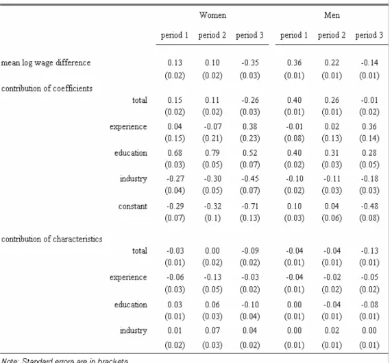
Results are reported in Table 2. The difference in mean (log) wages across countries and its evolution over time reflect the early statistical results of Section 2: the wage differential initially in favour of India has decreased over time and changed sign in the last period. For the first period (late 1980s), Table 2 shows that most of the difference seems to be explained by a price effect in favour of India, mostly driven by higher returns to education in this country. In the second period (mid-1990s), very little change seems to occur for the mean wage difference in the case of women. For men, however, the aforementioned increase in Chinese returns to education is responsible for a small change in the coefficient effect and, as a result, a decrease in the average Indo-Chinese wage difference.²² The difference in characteristics between Indian and Chinese workers plays no role for women and gives only a very small (and significant) advantage to Chinese wage earners in the case of men.

In the third period, the reversal of the wage gap in favour of China is mostly on account of a significant change in the coefficient effect, reinforced nonetheless by a significant change in endowment effect due to rapidly increasing education levels in China in the late 1990s/ early 2000s. The change in price effect is a combination of a strong decrease in returns to experience in China, more than compensated by the increased returns to education in this country (as documented in the previous section) and by a significant rise in the constant

20 The decomposition relies critically on the counterfactual mean X_I'β^ˆ_C, which represents a statistical estimate of the mean wage that people with the characteristics observed in the Indian distribution would have if remunerated according to the returns prevailing in China. It is clear, therefore, that this decomposition is a purely statistical exercise, since the counterfactual component does not account for economic response – either in partial or general equilibrium – to the “change” in returns. This is nonetheless a useful tool to quantify the respective roles of price versus composition effects as well as the specific role of key variables like experience or education.

21 The fit of the regression used for the decomposition are consequently smaller than what is reported in Tables A1 to A3 in the Appendix. For instance, OLS estimates for the first period give a R-square of .46 with specific controls and .45 without, in the case of India, and respectively .30 and .17 for China. The loss in goodness-of-fit is more important in China since regional dummies and communist party membership have significant impact on earnings (cf. Appleton et al., 2005, and Zhang et al., 2005).

22 We have checked that results were not exceedingly sensitive to the omitted group among educational dummies. Robustness check has also been conducted by using schooling years instead of education categories.

term.²³ Results are qualitatively the same for men and women, with small differences in levels and, precisely, slightly higher Indo-Chinese differentials for men.

Table 2: Decomposition of the Mean Indo-Chinese Wage Differential

5. Quantile Regression Decomposition

Since mean characteristics and returns to these characteristics can vary significantly across quantiles for a heterogeneous sample of individuals, it has become stylised in the literature to complete the previous exercise by a decomposition of differences in the entire distribution of wages. Precisely, we suggest hereafter to decompose the differential wage distribution illustrated in Figure 1 into endowment and coefficient effects, in a similar way as was done for the mean difference in equation (2).

A number of decomposition procedures have been suggested to untangle the sources of differences in wage distributions. Popular methods used in the wage inequality literature include the “plug-in” procedure of Juhn et al. (1993) based on parametric regressions, and the

23 The contribution of the intercept is difficult to interpret as it relates to the pay of those possessing the characteristics of the omitted categories (no experience, primary education, public administration). However, the cross-country difference in intercept must simply reflect a faster growth of the average labour productivity in China (at least, the part of it which is not capture by difference in returns to skill). This point is discussed further in the concluding section.

However, the increase in the constant term, especially between strong 1995 and 2002, also comes up in the estimations of Appleton et al. (2005, table 2) who use a slightly different specification. See the concluding section for further discussion.

semi-parametric procedure of DiNardo et al. (1996) based on sample reweighting. More recently, quantile-based decomposition methods have been suggested by Machado and Mata (2005) and Gosling et al. (2000). As demonstrated by Autor et al. (2005), the Machado-Mata approach nests most of the usual approaches and has been increasingly used in recent empirical applications.²⁴ The general idea is to estimate the whole conditional distribution by quantile regression and then to integrate this conditional distribution over the range of covariates in order to obtain an estimate of the unconditional distribution. It is then possible to estimate counterfactual unconditional distributions to perform usual decompositions, and in particular the two following counterfactuals: (i) the Chinese (log) earnings density function that would arise if Chinese wage earners had the same characteristics as their Indian counterparts (used to compute coefficient effects); and (ii) the density function that would arise if the Indian wage earners had the same returns to characteristics as the Chinese workers (used to compute endowment effects).

However, the Machado-Mata estimator is simulation-based, i.e. it combines quantile regression and bootstrapping to generate the two counterfactual density functions, so that estimations are quite slow. Also, ways to estimate the variance consistently have not been suggested. Recently, Melly (2006) has proposed to use moment conditions in order to derive an analytical estimator for the parameters of interest.²⁵ This estimator is faster to compute and can be used, in turn, to bootstrap results to provide standard errors. We opt for this approach in this paper.

Unfortunately, none of the above methods can be used to divide up the composition effect into the contribution of each single covariate, as can be done for the mean decomposition using the conventional Oaxaca-Blinder method (cf. Table 2). Machado and Mata (2005) suggest using an unconditional reweighting procedure to compute the contribution of covariate X to the composition effect. Unfortunately, as recently stated by Firpo et al (2007), doing so also changes the distribution of other covariates that are correlated with X.

Consequently, in what follows, we simply provide the decomposition of the total endowment and price effects without looking at the specific role of each covariate.

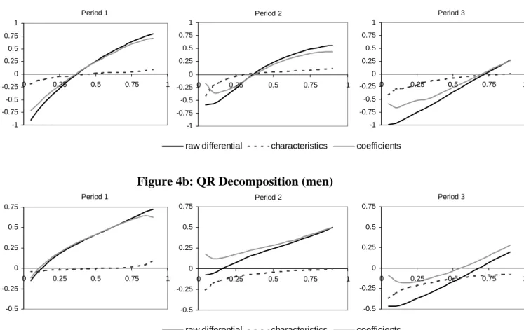
Figures 4a and 4b report the results of the decomposition for all three periods, obtained using the estimator of Melly (2006). Complete decomposition results for the median and the 25^th and 75^th deciles are reported in Table B in the Appendix together with bootstrapped standard errors.

Figures 4a and 4b firstly recall the overall trend encountered in Figure 1: a positive premium for Indian workers is observed in the first period, higher for men than women, and declines over time so that in the last period, Indian wage earners are better off than their Chinese counterpart only at the top of the distribution. The graphs also confirm results from the Oaxaca-Blinder decomposition: the positive wage gap in favour of India is mostly the result of the coefficient effect in the two first periods; there is no significant endowment effect except at the bottom of the distribution. There is little change between periods 1 and 2; we observe only a small narrowing of the cross-country wage gap, especially for top earners – which may be due to increased returns to seniority in China at this period, as previously explained – and stronger for men.

24 A detailed description of the estimator and an example of application is provided by Albrecht et al. (2003). Its asymptotic properties are studied in Albrecht et al. (2006) and Melly (2006).

25Results are numerically identical to those obtained with the Machado-Mata estimator if the number of simulations used in the latter procedure goes to infinity.

Things change in the third period with a strong decrease in the Indo-Chinese wage gap and a reversal in favour of China for the first three-quarter of the distribution. This shift is due to a combination of price and endowment effects, but the picture is naturally more complex than for the previous mean wage decomposition. Returns to characteristics now play in favour of China for the first half (two-third) of the male (female) distribution. This is partly explained by the rapid increase in Chinese returns to education, especially in lower quantiles (see Figure 3); yet, as previously documented, returns are still higher in India in the last period, which conveys that other factors must have come into play to explain the reversal.²⁶ The endowment effect is particularly strong for men and is unambiguously due to relatively higher education levels in China, especially in the lower part of the distribution. Table B in the Appendix confirms that this effect is significantly different from zero up to, at least, the 75^th centile.

Figure 4a: QR Decomposition (women)

Period 2

-1 -0.75 -0.5 -0.25 0 0.25 0.5 0.75 1

0 0.25 0.5 0.75 1

raw differential characteristics coefficients Period 1

-1 -0.75 -0.5 -0.25 0 0.25 0.5 0.75 1

0 0.25 0.5 0.75 1

Period 3

-1 -0.75 -0.5 -0.25 0 0.25 0.5 0.75 1

0 0.25 0.5 0.75 1

Figure 4b: QR Decomposition (men)

Period 2

-0.5 -0.25 0 0.25 0.5 0.75

0 0.25 0.5 0.75 1

raw differential characteristics coefficients Period 1

-0.5 -0.25 0 0.25 0.5 0.75

0 0.25 0.5 0.75 1

Period 3

-0.5 -0.25 0 0.25 0.5 0.75

0 0.25 0.5 0.75 1

Arguably, our estimates render only the average effect of each economic sector while compositions of characteristics and returns to these characteristics may vary from one sector to another. For this reason, we finally focus on two sectors in which each country is known to have comparative advantages, namely the manufacturing sector for China and the service sector for India.²⁷ These two sectors are large in both economies;²⁸ each of them is also sufficiently heterogeneous with respect to educational attributes or experience of the labourers. Focusing on these sectors then enable us to abstract to some extent from

26 As in the OLS decomposition, these unexplained factors must be capture in the intercepts.

27 According to Bosworth and Collins (2007), the post-1993 acceleration in growth in China was concentrated mostly in industry, which contributed nearly 60% of China’s aggregate productivity growth. In contrast, 45% of the growth in India in the second sub-period came in services.

28 In 2004, the share of the manufacturing (service) sector in the GDP was 39% (33%) in China and 16% (50%) in India.

unobserved industry effects and, at the same time, undertake the comparative analysis without loss of generality.

Results of the decomposition are reported in Figures 5a and 5b for men only (results for women are available upon request). They are qualitatively the same as for the whole urban economy. While endowment effects are virtually the same as before, there are only small differences in levels of the coefficient effects, and consequently of the overall wage gap; this certainly reflects different average productivity levels between countries. We take this result as an interesting robustness check of our more general findings but it also raises new questions that we keep for future research.

Figure 5a: Decomposition (manufacturing, men)

Period 2

-0.5 -0.25 0 0.25 0.5 0.75

0 0.25 0.5 0.75 1

raw differential characteristics coefficients Period 1

-0.5 -0.25 0 0.25 0.5 0.75

0 0.25 0.5 0.75 1

Period 3

-0.5 -0.25 0 0.25 0.5 0.75

0 0.25 0.5 0.75 1

Figure 5b: Decomposition (services, men)

Period 2

-0.75 -0.5 -0.25 0 0.25 0.5 0.75

0 0.25 0.5 0.75 1

raw differential characteristics coefficients Period 1

-0.75 -0.5 -0.25 0 0.25 0.5 0.75

0 0.25 0.5 0.75 1

Period 3

-0.75 -0.5 -0.25 0 0.25 0.5 0.75

0 0.25 0.5 0.75 1

5. Concluding Remarks

Despite the near simultaneous rise of China and India as major economic powers, there are few comparative studies of the two countries in terms of wage progression. In this paper, we undertake a comprehensive analysis of the Indo-Chinese wage differential in the urban sector between the late 1980s and the early 2000s. We attempt to describe how earnings distributions compare between countries at three points in time and to which extent ‘classical’

factors (education, experience) explain these differences.

Results can be summarized as follows. While Indian wages were higher in the late 1980s, faster productivity growth in China translates into faster wage progression such that, by the early 2000s, the wage gap is reversed in favour of this country at all levels except top earners.

Estimate-based decompositions of the mean wage difference show that the narrowing of the Indo-Chinese earnings gap is partly explained by rapidly rising returns to education in China in the late 1990s, especially at the bottom of the distribution. Interestingly, the reversal of the earnings gap for a large part of the distribution is accentuated by an increase in educational endowments in China. This shows that to some extent, voluntary policy impulse by the Chinese government have had an important effect, especially in improving the earnings capacity of the lower wage workers.

A critical aspect of the present study concerns the wage level comparisons between countries and at different periods. The PPP adjustments we made rely on estimates – taken from the World Development Indicators (WDI) – that were the only ones available until the recent period but which have been broadly criticised.²⁹ At the time we write this conclusion, preliminary results of the most recent 2005 round of International Comparison Program (ICP) just got published.³⁰ Milanovic (2007) provides an enlightening discussion about the new improvements and the consequences on measures of world inequality. The ICP preliminary report reveals in particular that the GDPs per capita of India and China were revised downward by 39.9% and 38.8% respectively compared to 2005 WDI. The reassuring aspect for the present study is that this correction is of very similar magnitude for both countries.

Anyhow, while it can be argued that absolute comparisons of earnings we made are dependent on the PPP adjustment method retained in the analysis, all other results and especially the dynamics of the wage differential on average and along the entire distribution remain valid.

A more puzzling aspect is the role of the intercept in the price effects highlighted in our decomposition. Especially between periods 2 and 3, intercepts have increased in both countries but much faster in China. Even if these terms are arbitrarily defined (in reference to the omitted categories) and difficult to interpret in absolute terms, the cross-country differences may be seen as reflecting unexplained productivity differences and in particular the faster growth in labour productivity in China. Additional variables that could explain some of this ‘average’ effect may not be easily introduced in this type of regression.³¹ This is in particular the case of institutional changes during the 1990s reform of state-owned enterprises in China; better ‘average’ performances in China are also attributed to higher capital intensity in the production processes and the more rapid TFP growth since the mid- 1990s.³² This could be seen as a limit to the exercise suggested in this paper. We believe, however, that the vocation of Mincer equation is maybe more to isolate the role of classical human capital variables (and their relative role in explaining wage differential across countries) than to explain labour productivity comprehensively. Nonetheless, and despite

29 Estimates of Chinese PPP exchange rates are based on a 1986 research study while estimates for India were based on extrapolations of the 1985 results of the International Comparison Program. See Milanovic (2007) for more details on these early estimates. See Dowrick and Akmal (2002) and Pogge and Reddy (2003), among others, on critical discussion on estimates of PPP exchange rates and the way those impede international comparisons and world inequality measures.

30 2005 International Comparison Program: Preliminary Results, 17 December 2007. Available at http://web.worldbank.org/WBSITE/EXTERNAL/DATASTATISTICS/ICPEXT/0,,menuPK:1973757~pagePK:

62002243~piPK:62002387~theSitePK:270065,00.html.

31 As argued in the text, one of the difficulty is the necessity to use a common set of covariates in Oaxaca- Blinder decompositions, which prevents from using important country-specific variables and necessarily reduce the fit of the Mincer model at use.

32 According to Bosworth and Collins (2007), slower TFP growth in India (compared to China and compared to the previous period) is due in part to rigid labour laws, which prevent the most efficient use of workers, and to a lack of modern infrastructure. Note also that our results in the last section, and in particular similar results in industry and service, convey that the rising tide lifts all boats in China. Even in the service sector, China seems to be more productive in the recent period (cf. also Bosworth and Collins, 2007), which drives the pattern in the Indo-Chinese differential of Figure 5b.

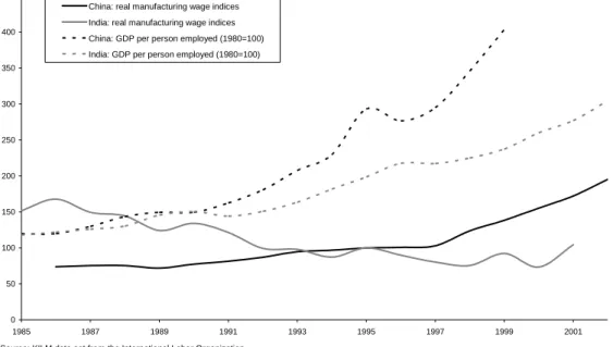
these difficulties, further research should attempt to better link micro and macro explanations to labour productivity. In Figure 6, we simply illustrate this point by plotting manufacturing wage indices and the GDP/capita for both countries over time. These alternative measures clearly show that the cross-country productivity gap has reversed in favour of China in the late 1980s, quickly followed by a reversal of the wage gap, and that these gaps have increased since then.

Figure 6: Other Indo-Chinese Comparisons of Wages and Labour Productivity

0 50 100 150 200 250 300 350 400 450

1985 1987 1989 1991 1993 1995 1997 1999 2001

China: real manufacturing wage indices India: real manufacturing wage indices China: GDP per person employed (1980=100) India: GDP per person employed (1980=100)

Source: KILM data set from the International Labor Organization

References

Albrecht, J., A. Bjorklund and S.C. Vroman. (2003): “Is there a glass ceiling in Sweden?”

Journal of Labor Economics, 21, 145-77.

Albrecht, J., A. van Vuuren and S.C. Vroman (2006): “Counterfactual distribution with sample selection adjustments: econometric theory and an application to the Netherlands”, Mimeo, Georgetown University, Washington, D.C.

Almeida dos Reis, J.G. and R. Paes de Barros (1991): “Wage inequality and the distribution of education: A study of the evolution of regional differences in inequality in metropolitan Brazil”, Journal of Development Economics, 36, 117–143

Appleton, S., L. Song, Lina and Q. Xia, (2005): “Has China crossed the river? The evolution of wage structure in urban China during reform and retrenchment”, Journal of Comparative Economics, 33:4, 644-663.

Autor, D, L. Katz and M. Kearney (2005): “Rising wage inequality: the role of composition and prices,” Working paper no. 11628, National Bureau of Economic Research, Cambridge, Massachusetts.

Blau, F. and L. Khan (1996): “International differences in male wage inequality: Institutions versus market forces”, Journal of Political Economy, 104(4), 791–837 (1996)

Blinder, A. S. (1973): “Wage discrimination: Reduced form and structural variables,”

Journal of Human Resources, 8, 436-455.

Bosworth, B. and S. A. Collins (2007): “Accounting for Growth: Comparing China and India”, Working Paper 12943, 2007, National Bureau of Economic Research, Cambridge, Massachusetts.

Bourguignon, F, F. Ferreira and P. Leite (2007): “Beyond Oaxaca–Blinder: Accounting for differences in household income distributions”, Journal of Economic Inequality, forthcoming.

Byron, R.P. and E.Q. Manaloto (1990): “Returns to education in China”, Economic Development and Cultural Change, 38(4), 783-796.

Demurger, S., M. Fournier, L. Shi and W. Zhong (2006): “Economic liberalisation with rising segmentation on China’s urban labour market”, Working paper no. WP 2006-46, ECINEQ – Society for the Study of Economic Inequality, Spain.

DiNardo, John, Fortin, Nicole, Lemieux, Thomas (1996): “Labor market institutions and the distribution of wages, 1973–1992: A semi-parametric approach”, Econometrica 64(5), 1001–1044.

Donald, S., D. Green, and H. Paarsch (2000): “Differences in wage distributions between Canada and the United States: An application of a flexible estimator of distribution functions in the presence of covariates”, Review of Economic Studies, 67, 609–633.

Dowrick, S.and M. Akmal (2005), “Contradictory Trends in Global Income Inequality: A Tale of Two Biases”, Review of Income and Wealth, 51 (2), 201-229.

Duraisamy, P. (2002): “Changes in returns to education in India, 1983-1994: By gender, age cohort and location”, Economics of Education Review, 21(6), 609-622.

Fields, G. (2005): “A Guide to Multisector Labor Market Models”, World Bank, mimeo.

Firpo, S., N. Fortin and T. Lemieux (2007): “Decomposing wage distributions using recentered influence function regressions”, working paper.

Gajwani, K., R. Kanbur and X. Zhang (2006): “Patterns of spatial convergence and divergence in India and China”, Paper prepared for the Annual Bank Conference on Development Economics (ABCDE), St. Petersburg, January 18-19, 2006.

Gosling, Amanda, Machin, Steve, Meghir, Costas (2000): “The changing distribution of male wages in the UK”, Review of Economic Studies, 67, 635–686

Heckman, J. J. and X. Li (2004): “Selection bias, comparative advantage and heterogeneous returns to education: evidence from China in 2000”, Pacific Economic Review, 9:3, 155-171.

Hyslop, Dean R., Maré, Dadid C. (2005): “Understanding New Zealand’s changing income distribution, 1983–1998: A semi-parametric analysis”, Economica 72, 469–495 Juhn, C, M. Kevin, B. Pierce (1993): “Wage inequality and the rise in returns to skill”,

Journal of Political Economy, 101(3), 410–442

Kijima, Y. (2006): “Why did wage inequality increase? Evidence from urban India 1983-99”, Journal of Development Economics, 81:1, 97-117.

Kingdon, G.G. and J. Unni (2001): “Education and women’s labour market outcomes in India”, Education Economics, 9(2), 173-195.

Knight, J. and L. Song (2003): “Increasing urban wage inequality in China”, Economics of Transition, 11:4, 597-619.

Koenker, R. and G. Bassett (1978): “Regression Quantiles”, Econometrica, 46:33-50

Liu, Z. (1998): “Earnings, education, and economic reforms in urban China”, Economic Development and Cultural Change, 46:4, 697-725.

Machado, J. and J. Mata (2005): “Counterfactual decomposition of changes in wage distributions using quantile regression”, Journal of Applied Econometrics, 20:4, 445- 465.

Maurer-Fazio, M. (1999): “Earnings and education in China's transition to a market economy Survey evidence from 1989 and 1992”, China Economic Review, 10:1, 17-40.

Melly, B. (2005): “Decomposition of differences in distribution using quantile regression”, Labour Economics, 12, 577-590.

Melly, B. (2006): “Estimation of counterfactual distributions using quantile regression”, working paper, university of St Gallen, SIAW.

Meng, Xin, Kidd, Michael P. (1997): “Labor market reform and the changing structure of wage determination in China’s state sector during the 1980s”, Journal of Comparative Economics 25, 403–421.

Milanovic, B. (2007): “An even higher global inequality than previously thought: A note on global inequality calculations using the 2005 ICP results”, mimeo.

Nguyen, B. T., J. Albrecht, S. C. Vroman and D. Westbrook (2007): “A quantile regression decomposition of urban-rural inequality in Vietnam”, Journal of Development Economics, 83:2, 466-490

Oaxaca, R. (1973): “Male-female wage differentials in urban labor markets”, International Economic Review 14, 693-709.

Pogge, T. W. and S. Reddy (2003), “Unknown: the extent, distribution, and trend of global income poverty”, July 26. Available at http://www.columbia.edu/~sr793/povpop.pdf.

Saha, B. and S. Sarkar (1999): “Schooling, informal experience, and formal sector earnings:

A study of Indian workers”, Review of Development Economics, 3(2): 187-199.

Wu, X. and W. Xie (2003): “Does the market pay off? Earnings returns to education in urban China,” American Sociological Review, 68(3), 425-442.

Zhang, J., Y. Zhao, A. Park and X. Song (2005): “Economic returns to schooling in urban China, 1988 to 2001”, Journal of Comparative Economics, 33:4, 730-752.

Appendix

Table A1: Estimates of Mincer equation (period 1: 1987-88)

Table A2: Estimates of Mincer equation (period 2: 1993-95)

Table A3: Estimates of Mincer equation (period 3: 2002-2004)

Table B: QR Decomposition