Addressing NGS Data Challenges: Efficient High Throughput Processing and Sequencing Error Detection

(1)

Addressing NGS Data Challenges: Efficient High Throughput Processing and Sequencing Error Detection

Inaugural-Dissertation

zur

Erlangung des Doktorgrades

der Mathematisch-Naturwissenschaftlichen Fakultät der Universität zu Köln

vorgelegt von

Amit Kawalia

aus Para Bass Suila, Alwar, Rajasthan (India)

Köln, 2016

(2)

(3)

Berichterstatter: Prof. Dr. Peter Nürnberg (Gutachter) Prof. Dr. Michael Nothnagel

Prüfungsvorsitzender: Prof. Dr. Hartmut Arndt Beisitzer: Dr. med. Holger Thiele

Tag der mündlichen Prüfung: 18/01/2016

(4)

(5)

Abstract

Next generation sequencing (NGS) technologies have facilitated the identification of disease causing mutations, which has significantly improved patient’s diagnosis and treatment. Since its emergence, NGS has been used in many applications like genome sequencing, DNA resequencing, transcriptome sequencing and epigenomics, to unfold the various layers of genome biology. Because of this broad spectrum of applications and recent decrement in cost, usage of NGS has become a routine approach to address many research as well as medical questions. It is producing huge amounts of data, which necessitate highly efficient and accurate computational analysis as well as data management.

This thesis addresses some of the challenges of NGS data analysis, mainly for targeted

DNA sequencing data. It describes the various steps required for data analysis including

their significance and potential negative effects on consecutive downstream analysis

and so on the final variant lists. In order to make the analysis more accurate and

efficient, an extensive testing of different bioinformatics tools and algorithms was

preformed and a fully automated data analysis workflow was developed. This workflow

is implemented and optimized on high performance computing (HPC) systems. I describe

different design principles and parallelization strategies that enable proper exploitation

of HPC resources to achieve high throughput of data analysis. Besides correcting for

known sequencing errors by using existing tools, this work is also aimed at the detection

of a new class of systematic sequencing errors called recurrent systematic sequencing

errors. I present an approach for the exploration of this class of errors and describe the

probable causes and patterns behind them. This includes some known and novel

patterns observed during this work. Furthermore, I provide a tool to filter the false

variants due to these errors from any variant list. Overall, the work performed during

this thesis has been already used (and will be used in future as well), to provide accurate

and efficient data analysis, which enables exploration of the genetic background of

various diseases.

(6)

(7)

Zusammenfassung

Die Next-Generation-Sequencing-(NGS)-Technologien haben die Identifizierung krankheitsverursachender Mutationen erleichtert, wodurch die Diagnose und Behandlung von Patienten deutlich verbessert wurde. Seit seiner Einführung wird NGS in vielen Anwendungsbereichen, wie Genom-Sequenzierung, DNA-Resequenzierung, Transkriptom-Sequenzierung und Epigenomik, eingesetzt, um die verschiedenen Ebenen der Biologie des Genoms zu entschlüsseln. Aufgrund dieses breiten Anwendungsspektrums und der aktuellen Kostensenkung ist die Verwendung von NGS zu einem Routineverfahren zur Bearbeitung vieler forschungsbezogener und medizinischer Fragestellungen geworden. Dadurch werden große Datenmengen erzeugt, die hoch effiziente und exakte computergestützte Analysen sowie ein entsprechendes Datenmanagement notwendig machen.

Diese Dissertation widmet sich einigen der mit der NGS-Datenanalyse verbundenen Herausforderungen, vor allem in Bezug auf die gezielte DNA-Sequenzierung ausgewählter genomischer Bereiche („targeted sequencing“ genannt). Sie beschreibt die verschiedenen für die Datenanalyse erforderlichen Schritte, ihre Bedeutung und potentiellen negativen Effekte auf anschließende Folgeanalysen und damit auf die finalen Variantenlisten. Um die Analyse exakter und effizienter zu machen, wurden umfassende Tests verschiedener bioinformatischer Tools und Algorithmen durchgeführt und ein vollautomatischer Analyse-Workflow entwickelt. Dieser Workflow ist auf Hochleistungsrechensystemen (HPC Systemen) implementiert und für diese optimiert worden. Ich beschreibe verschiedene Entwurfsprinzipien und Parallelisierungsstrategien, um eine gute Nutzung der Ressourcen eines HPC-Systems und hohen Durchsatz in der Datenanalyse zu erreichen. Neben der Korrektur bekannter Sequenzierungsfehler durch vorhandene Tools, widmet sich diese Arbeit auch der Detektion einer neuen Klasse systematischer Sequenzierungsfehler, „wiederkehrende systematische Fehler“ genannt.

Ich präsentiere ein neues Verfahren, um diese Fehlerklasse zu untersuchen und

beschreibe die ihr wahrscheinlich zugrundeliegenden Ursachen und Muster. Dabei

(8)

beobachtete ich einige bekannte und neue Muster. Weiterhin stelle ich ein Tool zur

Verfügung, um von diesen Fehlern verursachte falsche Varianten aus beliebigen

Variantenlisten zu filtern. Die während dieser Doktorarbeit durchgeführten und hier

präsentierten Arbeiten wurden bereits (und werden weiterhin) verwendet, um exakte

und effiziente Datenanalyse durchzuführen, die die Erforschung des genetischen

Hintergrundes verschiedenster Krankheiten ermöglicht.

(9)

Acknowledgement

I am very grateful to my supervisors Peter Nuernberg and Susanne Motameny who have given me an opportunity to work in the very exciting and challenging field of Next Generation Sequencing during this thesis. Special thanks to Susanne Motameny for extensive proofreading, moral support and guidance throughout my thesis. I also want to thank Holger Thiele who involved me in some other interesting projects and also supported me during the whole period. I would also like to thank Michael Nothnagel for his guidance, suggestions and for reviewing this work. Furthermore, I would like to thank Kamel Jabbari and Wilfried Gunia for their guidance and many fruitful conversations, both scientific and non-scientific. It has been a great pleasure to work with all of them.

Without their support and guidance throughout my work, this thesis would not have been accomplished.

I am also thankful to all other colleagues and my friends for their assistance and support.

I am also grateful to my parents and brother who believed in me and supported me

throughout my career. I cannot thank my wife enough who patiently supported and

helped me during my “low days” and tolerated my craziness.

(10)

(11)

List of Figures

Figure 1.1 Overview of Illumina sequencing (figure from (Mardis, 2013)). ... 23

Figure 1.2 Overview of Exome Sequencing (on Illumina sequencer). ... 27

Figure 1.3 Applications of WES and its impact on human health improvement. ... 29

Figure 2.1 Effect of quality trimming on our in-house data. ... 48

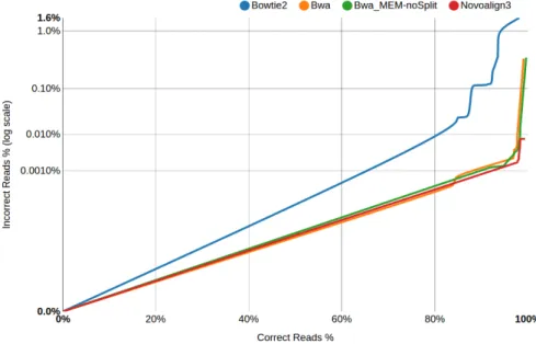
Figure 2.2 GCAT comparison of 4 different alignment algorithms. ... 52

Figure 2.3 Difference between the alignments produced by BWA-MEM and BWA-aln at n=7. ... 56

Figure 2.4 Difference between the alignments produced by BWA-aln at n=0.04, n=7 and n=10. ... 56

Figure 2.5 Improvement in the alignments after Indel realignment process. ... 61

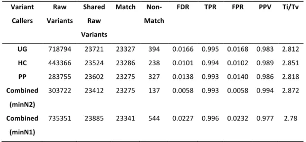
Figure 2.6 Overlap between raw variant lists of control sample NA12878 generated from 3 different variant callers. ... 64

Figure 2.7 Variant Qual score thresholds used during the comparison of individual callers and the integration approach. ... 65

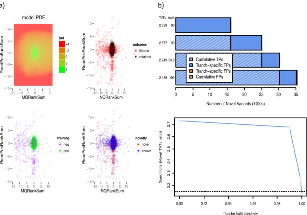
Figure 2.8 a) VQSR clustering based on 2 Annotations: ReadPosRankSum and MQRanksum. b) VQSR’s four- default tranches and their correlation with sensitivity and Ti/Tv ratio. ... 67

Figure 3.1 Automated workflow for exome sequencing data analysis. ... 80

Figure 3.2 Overview of HPC architecture. ... 82

Figure 3.3 Infrastructure surrounding the exome workflow. ... 83

Figure 3.4 Overview of workflow interaction with both CHEOPS and SUGI HPC systems. ... 84

Figure 3.5 Overview of workflow implementation at HPC. ... 85

Figure 3.6 Flow chart of the job submission function. ... 87

Figure 3.7 Performance of multi-threading with BWA-MEM and GATK HaplotypeCaller. ... 91

Figure 4.1 Alignment visualization of two systematic errors in a control sample (NA12878). ... 106

Figure 4.2 The four main components of the systematic error detection workflow. ... 110

Figure 4.3 Observed kmer construction from a sequence read. ... 111

Figure 4.4 Pileup format of aligned reads. ... 112

Figure 4.5 Distribution of errors throughout the genome captured by Prefix model (PM). ... 126

Figure 4.6 Distribution of errors throughout the genome captured by Suffix model (SM). ... 126

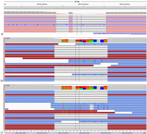
Figure 4.7 Alignment visualization by IGV in the MUC6 gene region. ... 128

Figure 4.8 Alignment visualization by IGV at location 11: 1016963 of MUC6 gene. ... 128

Figure 4.9 Sequence logos (from Weblogo tool) for 9mers at forward reference strand. ... 131

Figure 4.10 Alignment visualization of a systematic error by IGV. ... 132

Figure 4.11 MFE secondary structure of first (left) and last (right) 17mer from the list of top 25 17mers. 135

(14)

(15)

List of Tables

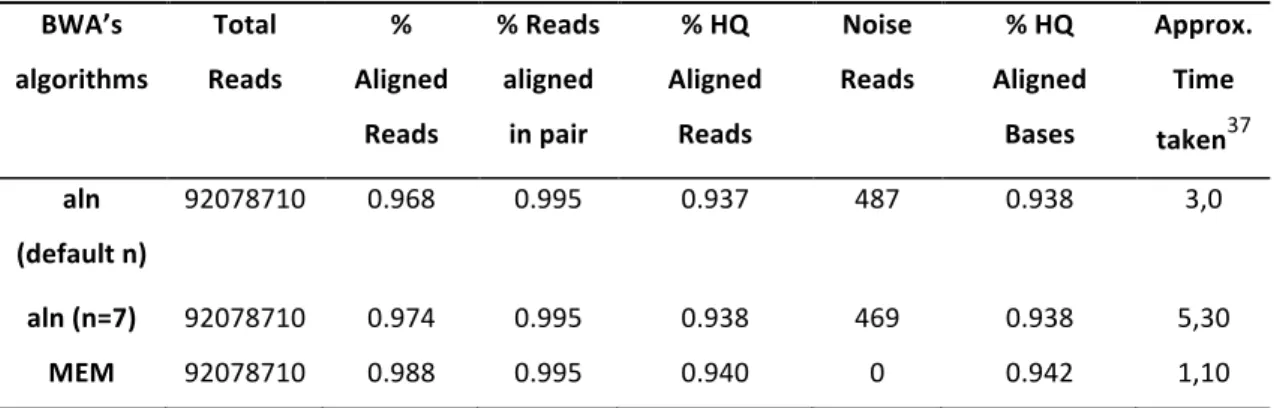
Table 2.1 Comparison between BWA’s alignment algorithms in context to reads alignment. ... 54

Table 2.2 Comparison between BWA’s alignment algorithms in context to called variants. ... 54

Table 2.3 Comparison of variants callers’ performance to the integrated approach. ... 64

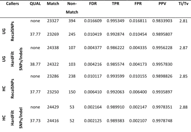
Table 2.4 Benchmarking results of different variant lists of control sample NA12878 with GIAB dataset. .. 73

Table 4.1 Statistics of generated 9mers from V2_IN. ... 121

Table 4.2 Overlap between the test dataset and the 3 other datasets. ... 121

Table 4.3 Overview of systematic errors in class 1: Platform dependent. ... 125

Table 4.4 Overview of systematic errors in class 2: Target enrichment dependent. ... 125

Table 4.5 List of genes having high RSEs and their paralogous genes. ... 129

Table 4.6 List of top 10 common motifs of length 3 (including known motifs occurrences) in RSEs associated 9mers in both upstream and downstream. ... 132

Table 4.7 List of top 25 17mers according to the nucleotide pairing probabilities (highest to lowest). ... 134

(16)

(17)

List of abbreviations

Abbreviation Term

AT Adenine Thymine

BAM Binary version of SAM

BP Base pair

BQSR Base Quality Score Recalibration

BWA Burrows-Wheeler Alignment

CHR Chromosome

CNV Copy Number Variation

CPU Central processing unit

DNA Deoxyribonucleic acid

DP Read depth

FDR False Discovery Rate

FN False negative

FP False positive

FPR False positive rate

GATK Genome Analysis Tool Kit

GB Gigabyte

GC Guanine Cytosine

HC Haplotype Caller

HDR High divergent region

HPC High Performance Computing

Indel Insertion or deletion

LCR Low complexity region

LIMS Laboratory Information Management System

MAF Minor allele frequency

MB Megabyte

MQ Mapping Quality

MSA Multiple Sequence Alignment

(18)

NGS Next Generation Sequencing

PCR Polymerase chain reaction

PM Prefix Model

PPV Positive prediction value

QC Quality Control

RAM Random-access memory

RSE Recurrent Systematic Error

SAM Sequence alignment format

SM Suffix Model

SNP Single Nucleotide Polymorphism

SSE Sequence Specific Error

STR Short tandem repeats

SV Structural Variation

TB Terabyte

TP True positive

TPR True positive rate

UG Unified Genotyper

VCF Variant Call Format

VQSR Variant Quality Score Recalibration

WES Whole Exome Sequencing

WGS Whole Genome Sequencing

XML Extensible Markup Language

(19)

Chapter 1 Introduction

Exploration of the causal gene variants underlying human diseases is one of the major interests of medical sciences. Recent advances in DNA sequencing technologies have enabled characterization of genomic landscapes of many diseases at significantly lower cost and in less time. The early identification of disease causing mutations has significantly improved patient’s diagnosis and treatment/therapy. Nowadays, DNA sequencing has become a routine work to address many research as well as medical questions in order to improve disease management.

The field of DNA sequencing has a very rich and diverse history (Rabbani, Mahdieh, Hosomichi, Nakaoka, & Inoue, 2012). The story of sequencing began, when Sanger’s studies of insulin first demonstrated that proteins are composed of linear polypeptides formed by joining amino acid residues (Hutchison, 2007; Sanger & Tuppy, 1951; Sanger, 1949). Shortly afterwards, the double-helical structure of DNA was proposed (Crick &

Watson, 1953), which raised the very significant question about DNA decoding (DNA to protein). However, due to the complexity of DNA, it took approximately 12 years to sequence the first gene (Holley et al., 1965).

In 1977, the first method for DNA sequencing through chain termination was developed

(Sanger, Nicklen, & Coulson, 1977). This method was quite slow and laborious which

prompted it’s automation (L. M. Smith et al., 1986). Automated Sanger sequencing

became the core technology of the Human Genome Project (HGP), funded in 1990, and

produced the first human genome draft sequences (Lander et al., 2001; Venter et al.,

2001). The HGP took 13 years to finish and was quite expensive which led to the

development of cheaper and faster next generation sequencing (NGS) technologies

(Mardis, 2008).

(20)

Introduction

NGS technologies, also known as high-throughput sequencing technologies, parallelize the sequencing process and produce millions of sequences simultaneously at relatively low cost. Taking advantage of these technologies, the 1000 Genomes Project could describe the genomes of 1,092 individuals from 14 populations. Aim of the project was to provide a catalogue of human genomic variation that was achieved by using a combination of low-coverage whole-genome and exome sequencing only in four years (Abecasis et al., 2012; The 1000 Genomes Project Consortium, 2010). After its emergence, NGS has been used in many applications to unfold the various layers of genetics and genome biology. In a research setting, it has been used for de novo genome sequencing, DNA resequencing, transcriptome sequencing and epigenomics.

Now, it has also become an asset of clinical diagnostic laboratories for patient care (Coonrod, Margraf, & Voelkerding, 2012).

Since the advent of NGS, there have been lots of improvements in the sequencing technologies like accuracy, read length and throughput. Moreover, the sequencing costs are also rapidly decreasing. Today NGS techniques are easily accessible and have become a preferred method in most of the research and diagnostics centres resulting in huge amount of sequencing data. The actual challenges are for the bioinformatics community to manage and analyse these data accurately and efficiently. In this work, I will address some of these issues that are relevant for targeted DNA sequencing. In the following sections, first I will provide an overview of NGS technologies. Then, I will provide an overview of targeted DNA sequencing methods and their applications in research and diagnostics. At last, I will briefly mention some data analysis terminologies followed by a description of the challenges of NGS data analysis and an overview of the thesis structure.

1.1 NGS technologies

There are many different platforms for massively parallel DNA sequencing: Roche/454

¹

, Illumina

²

, Ion Torrent

³

, PacBio RS

⁴

and Oxford Nanopore

⁵

. The first three: Illumina, 454

1

http://454.com/applications/index.asp This and other subsequent URLs are accessed on 26 August 2015.

(21)

NGS technologies

and Ion Torrent belong to the second generation sequencing technologies and are the most commonly used platforms in research and clinical labs today. The basic sequencing method of all of these platforms is sequencing by synthesis (SBS) (Hyman, 1988;

Turcatti, Romieu, Fedurco, & Tairi, 2008). In SBS methods, sequencing starts with a primer attached to the single stranded template DNA and proceeds with incorporation of a nucleotide base using a DNA polymerase. Every incorporated nucleotide is detected and the further extension, by means of the DNA polymerase, finally results in a complementary sequence to the template DNA (Berglund, Kiialainen, & Syvänen, 2011).

Although using the same SBS technology, these three platforms differ in the clonal amplification and nucleotide base detection process. Both 454 and Ion torrent use emulsion PCR amplification, whereas Illumina uses bridge amplification for the clonal amplification process (Margulies et al., 2005; Quail et al., 2012; Williams et al., 2006).

During the nucleotide base detection process, Illumina detects fluorescent signals emitted from nucleotide incorporation, whereas changes in pH and emission of light are detected by Ion torrent and 454 respectively (Mardis, 2008, 2013). Details of these technologies can be found in (Mardis, 2008, 2013; Metzker, 2010).

PacBio and Nanopore use recent sequencing technology known as third generation sequencing (Schadt, Turner, & Kasarskis, 2010). Both sequencing platforms perform single molecule sequencing in which sequencing is performed on single DNA molecule using single DNA polymerase without prior cloning or amplification step used in SBS methods. These techniques allow for more accurate sequencing in repetitive or low complexity regions (cf. Chapter 2) and are able to generate very long reads than the SBS technologies. However, currently these technologies are as matured as the second generation (e.g. Illumina) technologies, having high raw read error rates and low throughput. Moreover, there is a need to develop new sophisticated data analysis

2

http://www.illumina.com/systems/sequencing-platform-comparison.html

3

http://www.lifetechnologies.com/de/de/home/life-science/sequencing/next-generation- sequencing.html

4

http://www.pacb.com/products-and-services/pacbio-systems/

5

https://www.nanoporetech.com/

(22)

Introduction

algorithms, as these technologies posses different error profiles and different aspects of information in the generated sequencing data (Schadt et al., 2010). In our institute, we mainly use the Illumina sequencing technology and this work is also based on Illumina generated sequencing data. Thus, in the following section we provide a brief description of Illumina sequencing technology.

1.1.1 Illumina

Illumina is a widely used platform for DNA Sequencing, which uses clonal array formation and reversible terminator technology

⁶

(Bentley et al., 2008). Every DNA sequencing starts with library preparation (cf. Figure 1.1a) that includes DNA fragmentation, enzymatic trimming, fragment adenylation and adapter ligation (Mardis, 2013). After library construction, Illumina sequencing starts with cluster generation (the clonal amplification step) on the flow cell surface that includes binding of adapter ligated DNA templates to the oligos on the flowcell followed by repeated bridge amplifications (initiated by polymerases). This procedure results in clusters of co- localized clonal copies of each fragment (cf. Figure 1.1b). After that, each cluster is supplied with a polymerase and four fluorescently labelled nucleotide bases. Reversible terminator sequencing (cf. Figure 1.1c) starts with incorporation of all four bases in each cycle, but only adds one base per cycle at each cluster due to the blocking group attached at the 3’-OH position of the ribose sugar of the nucleotide base, which prevents incorporation of an additional base (Mardis, 2013). The incorporated nucleotide emits a fluorescent signal, which is detected and reported by image sensors.

Repetition of these cycles generates a sequence read from each cluster and thus yields millions of DNA sequences at the end. Illumina SBS technology supports both single-read and paired-end libraries. As the names suggest, single-read sequencing allows sequencing in one direction, whereas the paired-end approach performs sequencing from both ends of the DNA fragment. Nowadays, paired-end sequencing is mainly used as it provides better alignment across repetitive regions and also detects rearrangements such as insertions, deletions, and inversions.

6

http://www.illumina.com/documents/products/techspotlights/techspotlight_sequencing.pdf

(23)

NGS technologies

Figure 1.1 Overview of Illumina sequencing (figure from (Mardis, 2013)).

The Illumina platforms can be used for many different sequencing applications, such as whole-genome sequencing, de novo sequencing, candidate region targeted resequencing, DNA sequencing, RNA sequencing, and ChIP-Seq

⁷

. In order to support all of the mentioned applications adequately, Illumina provides four series of sequencers:

MiSeq, NextSeq, HiSeq, and HiSeqX, that vary in throughput, runtime, and cost. The selection of sequencer usually determined on the basis of the project’s requirements. At our institute, we use mainly HiSeq for exome sequencing and MiSeq for gene panel sequencing (or other target enrichment sequencing).

7

http://www.illumina.com/technology/next-generation-sequencing/sequencing-technology.html

(24)

Introduction

1.2 NGS applications

Next-generation sequencing has already many applications and it is still expanding. So far, it has been used in whole genome sequencing (WGS), targeted DNA sequencing (whole exome sequencing, gene panel sequencing, amplicon sequencing), transcriptome profiling (RNA-Seq), DNA-protein interactions (ChIP-Seq), etc. This thesis is focused on targeted DNA sequencing, thus only these applications will be described here.

1.2.1 Target enrichment methods

Though the sequencing cost has decreased significantly over the years and the goal of sequencing a whole genome for 1000 dollar is also achieved (at least partially

⁸

), still WGS is not routine work for most of the medium sized sequencing centres. Besides of high costs for obtaining approximately 30-fold coverage (i.e. sequencing each genomic position at least 30 times) of a human genome (generates approx. 90 Gb data in total), it needs a lot of computational resources to process and store this huge amount of data (Mamanova et al., 2010). Moreover, the whole genome contains both coding and non- coding part and due to the lack of annotations for the non-coding part, it is hard to interpret WGS data. Therefore, targeted enrichment methods are cost-effective alternates, allowing sequencing of selected genomic regions. There are mainly three different approaches to capture target regions: hybridization based, polymerase chain reaction (PCR) based and Molecular Inversion Probe (MIP). However, due to high cost and some coverage issues of MIP (Mamanova et al., 2010), hybridization or PCR based approaches are the commonly used methods for targeted DNA sequencing. I will describe these methods briefly here, a detailed comparison between them can be found in (Bodi et al., 2013; Kiialainen et al., 2011; Mamanova et al., 2010; Mertes et al., 2011).

PCR based capture

Polymerase chain reaction (PCR) based capturing of a genomic region of interest is a very traditional approach, which has already been used for Sanger sequencing. It has

8

It needs a specific setup of sequencers (HiSeq X Ten: http://www.illumina.com/systems/hiseq-x-

sequencing-system.html), which is very costly and out of the reach of medium sized sequencing centers.

(25)

NGS applications

also become ideal for the NGS applications that require to capture smaller targets approximately 10–100 kb in size (e.g. Gene panel sequencing). In brief, this approach starts with a target-specific primer design followed by a PCR reaction. This reaction can be a simple multiplex PCR (e.g. Ion AmpliSeq™ panels from Life Technologies, GeneRead DNAseq Gene Panels from Qiagen etc.), a micro-droplet PCR (RainDance), or array-based PCR (Access Array™ from Fluidigm) (Altmüller, Budde, & Nürnberg, 2014).

Hybridization based capture

These methods are faster and less costly than PCR based methods and used for the larger target size around 500 KB up to 65 MB (whole exome sequencing). They follow the basic principle of hybridization where baits (probes designed to match the target regions for sequencing) hybridize with a DNA library and pull down only fragments from the regions of interest. There are two different ways to execute this procedure: Micro- array based capture and solution based capture. In the first method, hybridization occurs on a micro-array chip where probes fixed to the chip surface hybridize to fragmented genomic DNA and immobilize complementary target sequences. On the contrary, solution based methods (Gnirke et al., 2009) use an excess of biotinylated DNA or RNA complementary probes (mobile probes in solution) to hybridize fragmented DNA. Then, streptavidin labelled magnetic beads are used to purify the target regions (Bodi et al., 2013). The solution based methods require less amount of DNA, and produce more uniform and specific sequences than the array-based method (Mamanova et al., 2010). Moreover, they do not need additional hardware (hybridization station) like the array-based methods. There are lots of commercial kits available based on this approach like SureSelect (Agilent), TruSeq (Illumina), SeqCap (NimbleGen), etc.

(Altmüller et al., 2014).

1.2.2 Whole exome sequencing (WES)

The ultimate goal of medical research is the identification of disease causing mutations to find therapeutic treatments or cures. It is known that the majority of the disease- causing mutations are located in coding and functional regions of the genome (Botstein

& Risch, 2003; Ng et al., 2009; Majewski, Schwartzentruber, Lalonde, Montpetit, &

(26)

Introduction

Jabado, 2011). Hence, sequencing of the complete coding regions (known as exome) has the potential to uncover causal mutations of genetic disorders (mostly monogenic), as well as predisposing variants in common diseases and cancers (Rabbani, Tekin, &

Mahdieh, 2014). Additionally, the exome constitutes only about 1% of the human genome. Therefore, it suffices to sequence approximately 64 MB, making exome sequencing a cost and time effective alternative for WGS (Ng et al., 2010).

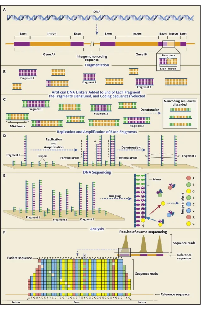
Overview of exome sequencing

In general, the sequencing process can be grouped into 3 stages: library preparation,

sequencing and imaging, and data analysis (Metzker, 2010). Library preparation is the

construction of the DNA templates required for DNA sequencing (Roe, 2004). It starts

with DNA isolation and fragmentation (cf. Figure 1.2-A and 1-B), followed by end- repair

and adapter ligation (cf. Figure 1.2-C) (Salomon & Ordoukhanian, 2015; Van Dijk,

Jaszczyszyn, & Thermes, 2014). Then, the library enrichment for exons (discard the

noncoding part) is performed by using target enrichment methods (mostly hybridization

based approaches (cf. Section “Hybridization based capture”)). Thereafter, PCR

amplification is usually performed to produce a sufficient amount of DNA template. As

the final product, library preparation generates the template molecules for amplification

on the flow cell surface (cf. Figure 1.2-D). After clonal amplification of the DNA

templates into clusters of identical molecules, sequencing starts on the flow cell with a

series of cycles. In each cycle, a complementary nucleotide labelled with one of four

coloured fluorescent dyes is added to each cluster of identical molecules (cf. Figure 1.2-

E). After identification of the fluorescent indicator of each cluster (by using a laser and

camera coupled to a microscope), the fluorescent indicator is removed, and the cycle is

repeated. Repetition of these cycles generates a sequence read of desired length

(usually 75 to 150 bp). During data analysis, sequence reads are aligned to a reference

DNA sequence followed by a genotype call for each position by using different

bioinformatics tools (cf. Figure 1.2-F) (Biesecker & Green, 2014). The nucleotide

detection procedure described above is for Illumina sequencing. Other technologies like

Ion Torrent or 454 can perform exome sequencing. Their sequencing procedures differ

mainly in clonal amplification and nucleotide detection (cf. Section 1.1).

(27)

NGS applications

Figure 1.2 Overview of Exome Sequencing (on Illumina sequencer). This figure is taken from (Biesecker &

Green, 2014).

(28)

Introduction

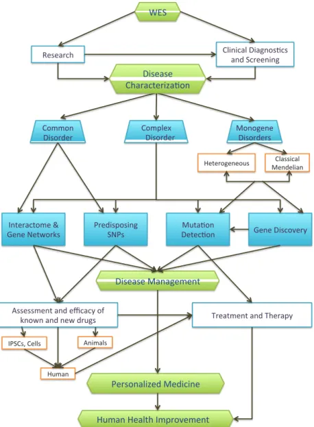
Applications of WES

It is already reported in many studies (Botstein & Risch, 2003; Ng et al., 2009) that the exome covers most of the functional variants including nonsense/missense mutations, small insertions/deletions, mutations that affect splicing and regulatory mutations (Rabbani et al., 2012). Hence, WES is a promising method to discover a significant number of disease causing variants and has been used in different areas of research as well as diagnostics (cf. Figure 1.3). In research settings, WES has the following main applications (Majewski, Schwartzentruber, Lalonde, Montpetit, & Jabado, 2011):

1. Characterization of monogenic disorders: WES is widely used to detect mutations causing monogenic inherited disorders. (Rabbani et al., 2012) presented a list of mendelian disease

⁹

genes identified (between 2010-2012) by exome sequencing and the numbers (102 studies) are significant enough to make WES a success story.

2. Identification of de novo mutations: De novo mutations are the extreme and more deleterious form of rare genetic variations (Veltman & Brunner, 2012). The case–parent trios sequencing is the most frequently used approach to detect this type of mutations (Chesi et al., 2013; Fromer et al., 2014; Vissers et al., 2010).

3. Uncovering the layers of complex disorders: After the success of WES for monogenic disorders, it also became an approach to identify causative variants in heterogeneous, complex diseases (Coonrod et al., 2012; Kiezun et al., 2013).

(Jiang, Tan, Tan, & Yu, 2013) reviewed the application of NGS in neurology and presented recent usage (studies from 2011-2013) of WES to identify rare variants in epilepsy, alzheimer, myotrophic lateral sclerosis, parkinson, spino cerebellar ataxias, and multiple sclerosis. Besides numerous applications in neurological disorders, WES is a helpful technique in some common complex disorders like

¹⁰

asthma (DeWan et al., 2012), diabetes (Shim et al., 2015; Synofzik et al., 2014), obesity (Paz-Filho et al., 2014; Thaker et al., 2015), etc. Moreover, it is also

9

Good explanation of mendelian disorders: http://www.nature.com/scitable/topicpage/mendelian-

genetics-patterns-of-inheritance-and-single-966

(29)

NGS applications

useful in cancer to find germline or somatic mutations (Ku et al., 2013; Ning et al., 2014; Pleasance et al., 2010).

Figure 1.3 Applications of WES and its impact on human health improvement. This figure provides an overview of exome sequencing usage in research and diagnostic settings. The overall aim of both researchers and clinicians is to explore diseases for better disease management, which can lead to personalized medicine for better cure/treatment. This figure is a modified version of the figure in (Rabbani et al., 2014).

Recently, clinicians also started using WES to establish diagnoses for rare, clinically unrecognizable disorders which might have a genetic background (Biesecker & Green, 2014; Coonrod et al., 2012; Need et al., 2012). As mentioned above, WES can find

WES

Clinical Diagnos/cs and Screening

Classical Mendelian Heterogeneous

Monogene Disorders Complex

Disorder Common

Disorder

Interactome &

Gene Networks

Disease Management

Human Health Improvement Assessment and eﬃcacy of

known and new drugs

Personalized Medicine

IPSCs, Cells Research

Predisposing

SNPs Muta/on

Detec/on Gene Discovery

Treatment and Therapy Animals

Human

Disease Characteriza/on

(30)

Introduction

causative variants, which facilitates understanding of the genetic mechanisms of these diseases. This can lead to gene-specific treatments or therapies like gene inclusion or replacement (Aiuti et al., 2009; Cavazzana-Calvo et al., 2010; Ott et al., 2006). WES can be also useful in prenatal diagnosis (PND), pre-implementation genetic diagnosis (PGD), prognosis of preclinical individuals, new-born screening procedures and treatment (Rabbani et al., 2014). It can also help in cancer by identifying driver mutations and genetic events leading to metastasis. This knowledge can be developed into treatments that prevent tumour recurrence or avoid therapeutic resistance (Majewski et al., 2011).

Altogether, WES can significantly contribute to personalized medicine and could improve human health by providing better disease management.

Limitations of WES

Besides, the enormous benefits of exome sequencing, there are a few drawbacks (Biesecker, Shianna, & Mullikin, 2011; Directors, 2012; Rabbani et al., 2014). Due to the target design and enrichment procedures, WES

1. is weak in structural variation detection.

2. does not cover certain sets of exons or provides less coverage for some exons, so that causal variants may be missed in some diseases.

3. can miss mutations in repetitive or GC rich regions and in genes with corresponding pseudogenes.

1.2.3 Gene panel sequencing

Gene panel sequencing is another type of targeted sequencing where genomic regions from a set of genes associated with a certain disease are targeted rather than the complete exome

¹¹

. There is prior knowledge about many diseases like their patho- mechanism or responsible genes, hence, sequencing of only those genes is sufficient and more cost and time effective than WES. Gene panel sequencing can use both hybridization based and PCR based target enrichment methods. It provides higher coverage (almost 100% of the target regions are usually covered sufficiently to call

11

Sequencing overview is almost the same as in WES except for a possibly different target capture.

(31)

NGS applications

variants), specificity, and uniformity than WES, which are essential for confident variant detection, especially for low-frequency variants (e.g., mutations only present in a small subset of cells in a tumour sample). Therefore, gene panel sequencing is gaining popularity both in research and diagnostic settings (Altmüller et al., 2014; Glöckle et al., 2013; Lynch et al., 2012; Rehm, 2013; Sie et al., 2014; Sikkema-Raddatz et al., 2013;

Wooderchak-Donahue et al., 2012).

Due to its high accuracy, medical centres are making different gene panels for diagnostic purpose. In this context, a brief overview of applications of gene panels and a list of clinically available disease-targeted tests has been reported by (Rehm, 2013). Moreover, (Sikkema-Raddatz et al., 2013) claims that targeted sequencing can replace Sanger sequencing in clinical diagnostics. They compared results from a panel of 48 genes associated with hereditary cardiomyopathies with Sanger sequencing and achieved approximately 100% reproducibility. This study concludes that this panel can be used as a stand-alone diagnostic test. In another study (Consugar et al., 2014), gene panel sequencing was used for genetic diagnostic testing of patients with inherited eye disorders. They designed a genetic eye disease (GEDi) test in this study with high sensitivity and specificity (97.9 and 100% respectively).

In cancer research and diagnosis, gene panel sequencing (or amplicon sequencing) has also been used for many studies to uncover somatic and germline mutations (Dahl et al., 2007; De Leeneer et al., 2011; Harismendy et al., 2011; Meldrum, Doyle, & Tothill, 2011). (Laduca et al., 2014) used four hereditary cancer panels (breast panel, ovarian panel, colon panel, and cancer panel) for diagnosis of hereditary cancer predisposition (Laduca et al., 2014). There are also many commercially available standard cancer panels or other gene panel like Illumina TruSight

¹²

, Illumina TruSeq, Amplicon Cancer Panel

¹³

or Ion AmpliSeq Cancer Hotspot Panel v2

¹⁴

which can be used routinely in both research and clinical settings (Tsongalis et al., 2014). A brief list of standard and customized gene

12

http://www.illumina.com/products/trusight-panels.html

13

http://www.illumina.com/products/truseq_amplicon_cancer_panel.html

14

https://www.lifetechnologies.com/order/catalog/product/4475346

(32)

Introduction

panels can be found in (Altmüller et al., 2014). Moreover, the most recent development in this direction is the “Mendeliome”, which is a set of approximately 3000 Mendelian genes known to cause human diseases (Alkuraya, 2014).

1.3 Basic terminologies in data analysis

This section contains definitions of the few terms that are required to understand the content of following sections. Some other terminologies will be defined during their usage throughout the other chapters.

Fastq: It is a text-based file format

¹⁵

, containing sequence reads and the quality score of every base of the read.

Read: It is a raw sequence (string of the letters A,C,G,T,N) generated from a sequencing machine.

Insert size: In paired-end sequencing, the insert size is the length of the sequenced DNA fragment. It can be computed from the alignment as the length of read1 plus the length of read2 plus the distance between them.

Read alignment: It is alignment (or mapping) of reads from a sequenced DNA on the reference genome sequence, to identify the differences or regions of similarity between both sequences. In general, there are two basic types of alignment:

• Global alignment: This is the alignment between entire sequences of approximately equal size. The Needleman–Wunsch algorithm (Needleman &

Wunsch, 1970) is the general algorithm for this type of alignment. By using dynamic programming

¹⁶

, it breaks the sequences into different parts and tries to align them. Then the algorithm searches for an optimal alignment of the complete sequence based on all sub-alignments.

15

http://en.wikipedia.org/wiki/FASTQ_format

16

http://en.wikipedia.org/wiki/Dynamic_programming

(33)

Basic terminologies in data analysis

• Local alignment: As the name suggests, local alignment tries to find the most similar part/section between two sequences instead of mapping the entire sequences. The basic algorithm for this purpose is the Smith-Waterman algorithm (T. F. Smith & Waterman, 1981), which is another significant application of dynamic programming.

SAM/BAM: SAM stands for Sequence Alignment Format

¹⁷

and BAM is its compressed (encoded) format. SAM is a tab-delimited format (generated after alignment) containing all necessary information related to the alignment of sequencing reads on the reference sequence, e.g. mapping position, mapping quality, sequence reads and their base quality scores etc.

VCF (Variant Call Format): It is a tab-delimited text file format to store sequencing variants with a certain set of information (Danecek et al., 2011) (e.g. position in genome, type of variant, variant supporting evidences etc.).

Coverage: It can be described in two different ways: read coverage and sample coverage. A read coverage (also called read depth) is the number of reads aligning at a specific genomic location. Sample coverage is the average read coverage across all genomic locations targeted during a sequencing experiment. Sample coverage can be represented by values like 10x, 20x, 30x, which means the average read depth is 10, 20, 30, respectively.

Base quality score (Q): It is also known as a phred score (Q) as it is calculated by the Phred algorithm (Ewing & Green, 1998; Ewing, Hillier, Wendl, & Green, 1998). It represents the probability that a base is miscalled. If P is the estimated error probability for a base-call, then the phred score is calculated as follow:

𝑄 = −10 log

_!"

𝑃

17

https://samtools.github.io/hts-specs/SAMv1.pdf

(34)

Introduction

Mapping quality score (MQ): It is a phred score which represents the probability that a read is misaligned on the reference (H. Li, Ruan, & Durbin, 2008). If P is the estimated error probability for a misalignment, then the mapping quality can be calculated as follow:

𝑀𝑄 = −10 log

_!"

𝑃

Variant quality score (Qual): It is also a phred score like MQ and Q and describes the probability of a called base being an alternate allele. If P is the posterior probability P(g|D) of the called genotype g given the observation D, then Qual can be calculated as (H. Li et al., 2008):

𝑄𝑢𝑎𝑙 = −10 log

_!"

(1 − 𝑃)

For all the quality scores (Q, MQ, Qual), a high phred score means that the examined site has low error probabilities and vice-versa.

Specificity and Sensitivity: In general, specificity estimates the fraction of correctly identified negatives (e.g. wrong outcome), whereas sensitivity estimates the fraction of correctly identified positives (e.g. true outcome)

¹⁸

. In this thesis, these terms will be used in two different contexts: variant calling and alignment. Definition of these terms in the context of alignment can be found in Chapter 2 (where these terms have been used for the first time). In the variant calling context, specificity and sensitivity, also known as true negative rate and true positive rate, are measures of the accuracy and the ability to detect a variant of a variant caller, respectively, and can be calculated as follows:

Sensitivity or true positive rate (TPR)= TPs (TPs + FNs) Specificity or true negative rate (TNR)= TNs (TNs + FPs) False positive rate (FPR) = 1- Specificity

True positives (TPs): These are the real variants, also called by the variant caller.

False positives (FPs): These are variants that are called by the variant caller but are not the real variants.

False negatives (FNs): These are real variants that are not called by the variant caller.

18

https://en.wikipedia.org/wiki/Sensitivity_and_specificity

(35)

Challenges in NGS data analysis

True negatives (TNs): These are variants that are not real, and also not called by the variant caller.

1.4 Challenges in NGS data analysis

The rapid fall in sequencing cost expanded the usage of NGS techniques, which resulted in huge amounts of data. Now it’s turn for the Bioinformatics community to make sense of these data. There are many challenges, which need to be addressed carefully. They can be categorized mainly in two parts: Efficient data processing and accuracy of results.

The challenges belonging to each category are briefly described below.

1.4.1 Efficient data processing

NGS technologies are high-throughput in nature that means they produce huge amounts of sequencing data in a relatively short time. The amount of data can be categorized in two different sections: first data produced by a single sequencing run for a sample and secondly data produced by a study containing certain set of samples. In both of these categories, the amount of data generated is increasing rapidly. Thus, the data processing and management is a major challenge and should be able to address all requirements for different applications.

In order to obtain relevant findings from the raw data, it needs to go through various stages like data cleaning, sequence alignment, variant calling, etc. There are plenty of algorithms for these individual tasks but in order to run them fast, they need to be stitched together in the correct order. This workflow can be very complex and needs enough resources or high performance computing (HPC) for smooth operation.

Moreover, it should be automated to reduce the manual efforts and chances of manual errors during data analysis operations.

Nowadays, almost every automated NGS workflow uses HPC clusters. Here, the power

of multiple CPUs can be used in a massively parallel way to finish tasks that would take a

couple of days on a single CPU in a couple of hours. For example, the MegaSeq

(36)

Introduction

(Puckelwartz et al., 2014) and HugeSeq (Lam et al., 2012) workflows use HPC for whole genome sequencing data analysis. These workflows utilize the MapReduce

¹⁹

approach to speed up the data analysis. In the MapReduce approach, first data is split into chunks and then processed in parallel followed by merging of the results. We also use the MapReduce approach to speed up our exome workflow. Existing automated workflows can be Linux-based frameworks implemented on HPC systems via bash

²⁰

scripts like NGSANE (Buske, French, Smith, Clark, & Bauer, 2014) or our exome workflow.

Additionally, they can be available in form of a web-interface like WEP (Antonio et al., 2013) or a VirtualBox and Cloud Service like SIMPLEX (Fischer et al., 2012), enabling users with little bioinformatics knowledge to analyse their data on remote HPC systems.

All of these above-mentioned examples show the necessity of workflow implementation on HPC systems to speed up NGS data analysis and also provide some details of the HPC implementation and parallelization strategies. However, besides the speed of a workflow, its stability, robustness and maintainability are also important concerns. An automated workflow should be fast, stable and robust as well as easy to maintain. The automation of the workflow and its implementation (with consideration of the above mentioned principles) on HPC comes with many challenges, which will be described in Chapter 3.

1.4.2 Accuracy of results

Downstream analysis of sequencing data can be significantly affected by the accuracy of results. Error propagation during data processing may lead to false positives (FPs) and misleading findings. On the other hand, badly selected strategies/tools can lead to false negatives, which means loss of true variants. These undetected variants might be the causative ones or can lead to uncover additional layers of some diseases, thus, this problem is more severe than FPs. Therefore, to find a proper balance between accuracy and sensitivity of results is another significant challenge for data analysis, which will be described in Chapter 2.

19

https://www.usenix.org/legacy/event/osdi04/tech/dean.html

20

http://tiswww.case.edu/php/chet/bash/bashtop.html

(37)

Challenges in NGS data analysis

Although, there are different alignment algorithms accompanied with post alignment improvements and different variant callers with reasonable accuracy. However, getting a variant list containing only true variants is still a challenge and false positive calls (FPs) remain a problem. Some of the FPs are due to the limitations of current tools, however, random sequencing errors and sequencing biases are other major contributors.

Sequencing biases can be categorized in three main classes coverage bias, batch effects and systematic errors (Taub, Corrada Bravo, & Irizarry, 2010; Yang, Chockalingam, &

Aluru, 2013).

Coverage bias

Coverage bias means non-uniform coverage throughout the sequenced genomic locations. Genomic locations containing low-complexity regions

²¹

like GC-rich sequences are the major source of coverage bias, that is non-uniform coverage or even no coverage in these regions (Sims, Sudbery, Ilott, Heger, & Ponting, 2014). (Dohm, Lottaz, Borodina, & Himmelbauer, 2008) first studied the effect of the unbalanced GC content of a genome (known as GC bias) on read coverage and found lower read coverage in GC or AT rich regions. Soon after, Kozarewa and colleagues showed that amplification artefacts introduced during the library preparation are the major source of the heterogeneous distribution of the read coverage (Kozarewa et al., 2009). After that, the GC bias effect has been studied many times in different contexts with similar observations (Aird et al., 2011; Chen, Liu, Yu, Chiang, & Hwang, 2013; Chilamakuri et al., 2014; Clark et al., 2011; Lan et al., 2015). During the library preparation, the PCR step yields lower amplification of regions with high GC or high AT content which results in lower sequencing coverage (Clark et al., 2011). Moreover, the GC bias reduces the efficiency of capture probe hybridization that also leads to lower read coverage (Chilamakuri et al., 2014). This reduced read coverage might result in many false positive (FPs) or false negative (FNs) variant calls (cf. Chapter 2). For example, low coverage at a certain region can be detected as a copy number variant (e.g. deletion) although it is just

21

DNA regions having biased nucleotide composition and enriched with simple sequence repeats.

(38)

Introduction

because of the GC effect. Similarly, some true variant might be missed or filtered out due to the minimum coverage threshold filter used during variant calling.

Because of the prevalent knowledge about the effect of GC bias, there are many ways to avoid or correct this effect. It can be avoided either during the library preparation (Aird et al., 2011; Kozarewa et al., 2009; Oyola et al., 2012) or compensated during the downstream analysis of sequencing data. (Benjamini & Speed, 2012; Cheung, Down, Latorre, & Ahringer, 2011) provided the “GCcorrect” tool and BEAD algorithm, respectively, that perform different normalization techniques for GC bias correction.

Moreover, most of the copy number calling tools based on the depth of coverage approach (Medvedev, Stanciu, & Brudno, 2009) perform read depth normalization to correct for the GC bias (Alkan et al., 2009; Fromer et al., 2012; Krumm et al., 2012;

Plagnol et al., 2012).

Batch effect

“Batch effects are sub-groups of measurements that have qualitatively different

behaviour across conditions and are unrelated to the biological or scientific variables in

a study” (Leek et al., 2010). Thus, the different batches of a sequencing experiment can

have errors that are due to the technical or manual variability. For example, usage of

different lots of reagents, chips or instruments can introduce variability between

different batches of sequencing experiments. Moreover, the individual experience of

different technicians handling the samples during the library preparation and

sequencing process can also result in batch effects. Batch effects can easily lead to some

false discoveries or conclusions. Leek and colleagues has summarized the consequences

of batch effects and also demonstrated the presence of batch effects in sequencing data

from the 1000 genomes project (Leek et al., 2010). Moreover, they also provided

solutions to avoid batch effects. Careful study design and some statistical solutions

(exploratory statistical analysis) can easily eliminate the consequences of batch effects

(Leek et al., 2010).

(39)

Challenges in NGS data analysis

Systematic error

Systematic error is the error introduced by the sequencing platform that follows some systematic patterns instead of a random distribution. Systematic errors can be classified as position specific and sequence specific (Meacham et al., 2011). Position specific error is the class of errors where the error (i.e. mismatch) occurs mostly at certain genomic positions or in certain regions of the reads (e.g. base calling errors towards the 3’ end).

In contrast, the sequence specific error is surrounded (upstream or downstream of the error position) by a certain sequence motif (consecutive nucleotide bases of a certain length).

As Illumina sequencing is the most widely used technology, lots of studies have been performed to understand errors generated from these sequencers. It has been observed that Illumina generates more substitution errors than Indel errors (Dohm et al., 2008).

Dohm et al. observed that most of the subsititution errors are either persent at the ends

of reads (esp. at the 3’ end) or in the GC-rich regions. They found that the nulceotide

base A is substituted by C and C is substituted by G more often then the other types of

base susbtituion. (Kircher, Stenzel, & Kelso, 2009) studied these base calling errors and

found that these errors are more frequent during the first and the last cycles. They

observed that the base calling errors are more frequent in the later cycles due to the

effects of crosstalk, declining intensities, pre-phasing and phasing, and accumulation of

the “T” nucleotide. (Metzker, 2010) reviewed different NGS techonlogies and also

reported that the lagging-strand dephasing is the main cause of this type of sustitution

errors in Illumina data. Dephasing means loss of synchronicity of growing primers for

any given cycle during clonal amplification process (Metzker, 2010). In another word,

when the blocking effect of the 3’-OH group (which allows the next nucleotide base

incorporation) (cf. Chapter 1) does not work (or still works in the next cycle), some

copies of the DNA template lose synchronization with the other copies of DNA template

belonging to the same cluster (e.g. incorporation lags one base behind the rest of

cluster). It can be referred in two ways: lagging strand dephasing and leading strand

dephasing. The lagging strand dephasing refers to the incomple extension of a template

ensemble becuase of lagging behind compared to the rest of the cluster as mentioned

(40)

Introduction

above. In contrast, leading-strand dephasing is the incorporation of more than one nucleotide in a given cycle (Metzker, 2010). Based on the available knoweldege, lots of improvement has been performed like improvements in the sequencing chemistry and the base calling algorithms. Moreover, recent alignment and variant calling algorithms are also aware of this type of error. Moreover, some standard filtering strategies are also able to filter FPs generated by these errors. However, there is still lots to explore in this class of error as many systematic errors are hard to detect or not detected so far.

Thus, Chapter 4 is dedicated to the exploration of systematic errors.

1.5 Thesis organization

As mentioned above, NGS data analysis comes with certain challenges. This thesis is aimed to address some of these challenges to enhance the efficiency and accuracy of DNA sequencing data analysis. The work presented in thesis is my own work except Chapter 3, which is joint work of Dr. Susanne Motameny and myself.

In Chapter 1, I have provided an overview of NGS technologies, targeted DNA sequencing methods and their applications. I have briefly mentioned some data analysis terminologies followed by a description of the main challenges of NGS data analysis.

Chapter 2 provides an overview of the data analysis steps of targeted sequencing as implemented in our data analysis workflow. It contains details of essential steps (including their significance) required to generate a variant list from raw sequencing data. It also describes the possible adverse effects of each step (if used inappropriately) and highlights the limitations of the applied algorithms. Moreover, it demonstrates the importance of the selection of appropriate tools and associated parameter settings in terms of both accuracy and efficiency. Furthermore, it provides an overview of filtering and benchmarking strategies applied in our data analysis workflow to achieve a good balance between accuracy and sensitivity of the results.

In Chapter 3, details of our in-house developed automated data analysis workflow are

provided. The aim was to avoid manual repetition of all of the data analysis steps as

(41)

Thesis organization

mentioned in Chapter 2 and thus to save time for downstream analyses of data and its validation. Fast and efficient automated data processing requires a large amount of computational resources that necessitates its implementation on high performance computing (HPC) clusters. However, HPC comes with some challenges and requires certain workflow design principals as parallelization strategies and some other tricks.

This chapter provides details of these design principals and strategies, which gave our workflow speed, stability and robustness while keeping it easy to maintain.

Chapter 4 is dedicated to an important but hard to detect class of sequencing errors:

Systematic Sequencing Errors (SSEs), which can easily damage the accuracy of the results. The chapter presents a novel approach to explore SSEs. During the error exploration, reproducible error behaviour in different datasets has been observed which led to a newly coined class of errors: “Recurrent Systematic Errors (RSEs)”. The characteristics of RSEs and some of the known and novel patterns behind this type of error are described in this chapter. Moreover, an RSE filtering tool “FilterRSEs” has been developed, which can filter FPs (due to RSE) from a given variant list (VCF file). It uses the detected RSE location and associated annotations to provide different filtering options.

Chapter 5 concludes the thesis with a discussion of the findings and an outlook on current and future developments.

1.5.1 Relevant publications

The following publications related to this thesis have been published:

• Leveraging the Power of High Performance Computing for Next Generation Sequencing Data Analysis: Tricks and Twists from a High Throughput Exome Workflow. Amit Kawalia, Susanne Motameny, Stephan Wonczak, Holger Thiele,

… Ulrich Lang, Viktor Achter, Peter Nürnberg. PLOS ONE (2015)

• Rare variants in γ-aminobutyric acid type A receptor genes in rolandic epilepsy

and related syndromes. Reinthaler EM, Dejanovic B, Lal D, Semtner M,

(42)

Introduction

…Kawalia A…EuroEPINOMICS Consortium, Nürnberg P, Lerche H, ….Neubauer BA, Zimprich F. Annals of Neurology (2015)

• Homozygous and compound-heterozygous mutations in TGDS cause Catel- Manzke syndrome. Ehmke N, Caliebe A, Koenig R, Kant SG, …, Kawalia A…Nürnberg P, Siebert R, Manzke H, Mundlos S. American Journal of Human Genetics (2014)

• Mutations in STX1B, encoding a presynaptic protein, cause fever-associated epilepsy syndromes. Schubert J, Siekierska A, Langlois M, May P, …Kawalia A…Nürnberg P, Crawford AD, Esguerra CV, Weber YG, Lerche H. Nature Genetics (2014)

• DEPDC5 mutations in genetic focal epilepsies of childhood. Lal D, Reinthaler EM,

Schubert J, …Kawalia A…Nürnberg P, Sander T, Weber Y, Zimprich F, Neubauer

BA. Annals of Neurology (2014)

(43)

Chapter 2 Accurate DNA sequencing data analysis:

hurdles and solutions

Almost every day, sequencers produce huge amounts of DNA sequencing data containing millions of sequencing reads. Raw data coming out from these machines contain only sequencing reads and their quality scores. Each sequencing read is just a series of four letters (A, T, G, C) representing the four nucleotides (adenine, thymine, guanine, cytosine, respectively) and does not provide any significant information in its original state. To make sense of these raw sequencing data, they need to go through various bioinformatics analyses. Conversion of a raw sequencing file (fastq file) into a variant list (VCF file) requires certain data processing steps (Van der Auwera et al., 2013) that can be mainly categorized into 4 different sections: pre-processing, alignment, variant calling, and functional annotation.

All of these analysis steps are interconnected, build on each other, and usually involve running some tool or script. Thus, every analysis step can affect its consecutive analysis in an adverse manner if not used appropriately. For example, discarding bad quality data during the quality control step can improve the specificity of results. However, this can lead to loss of data and hence lower sensitivity of results. Similarly, selection of wrong tools/algorithms with their default (or inappropriate) parameter settings can also lead to bad specificity or sensitivity. Both of these situations are harmful for the final results and can mislead variant discovery. Less specific results contain lots of false positives, which make detection of true variants complicated. On the contrary, less sensitive results can lead to the absence of some true variants in the final variant list. Thus, finding a proper balance between specificity and sensitivity of results is very important.

This chapter aims to address these issues in order to achieve a good balance between

sensitivity and specificity of the results (cf. Section 1.3). It provides a description of the

main steps of DNA sequencing data analysis, their significance and the possible adverse

Addressing NGS Data Challenges: Efficient High Throughput Processing and Sequencing Error Detection