Aufsätze zur Selbstselektion und zum Messemanagement

Aufsätze zur Selbstselektion und zum Messemanagement

Inauguraldissertation zur

Erlangung des Doktorgrades der

Wirtschafts- und Sozialwissenschaftlichen Fakultät der

Universität zu Köln

2010

vorgelegt von

Dipl.-Kff. Sabine Scheel-Kopeinig aus

Villach, Österreich

Referent: Prof. Dr. Karen Gedenk

Korreferent: Prof. Dr. Franziska Völckner

Tag der Promotion: 23. Juli 2010

Inhaltsverzeichnis

Abbildungsverzeichnis ... VI  Tabellenverzeichnis ... VII Abkürzungsverzeichnis ... VIII Symbolverzeichnis ... XI

ÜBERBLICK ... 1 

Abschnitt A:

Caliendo, Marco/Kopeinig, Sabine: Some Practical Guidance for the

Implementation of Propensity Score Matching ... 6

1. Introduction ... A.1

2. Evaluation Framework and Matching Basics ... A.3

3. Implementation of Propensity Score Matching ... A.7

3.1 Estimating the Propensity Score

... A.7

3.2 Choosing a Matching Algorithm

... A.11

3.3 Overlap and Common Support

... A.15

3.4 Assessing the Matching Quality

... A.17

3.5 Choice-Based Sampling

... A.19

3.6 When to Compare and Locking-in Effects

... A.20

3.7 Estimating the Variance of Treatment Effects

... A.21

3.8 Combined and Other Propensity Score Methods

... A.24

3.9 Sensitivity Analysis

... A.26

3.10 More Practical Issues and Recent Developments

... A.29

4. Conclusion ... A.32

References ... A.38

Abschnitt B:

Caliendo, Marco/Clement, Michel/Papies, Dominik/Scheel-Kopeinig, Sabine: The Cost Impact of Spam-Filters: Measuring the Effect of

Information System Technologies in Organizations ... 7

Introduction ... B.4

Related Research ... B.8

Method ... B.10

Research Design and Data ... B.13

Central Costs

... B.14

Individual Measures

... B.15

Cost Analysis ... B.18

Group Characteristics before Matching

... B.18

Propensity Score Estimation

... B.18

Matching Results

... B.20

Effect Heterogeneity

... B.22

Sensitivity to Unobserved Heterogeneity

... B.23

Conclusion and Limitations ... B.25

References ... B.27

Abschnitt C:

Kopeinig, Sabine/Gedenk, Karen: Make-or-Buy-Entscheidungen von Messegesellschaften ... 8

1. Problemstellung ... C.3 2. Relevante Make-or-Buy-Fragestellungen ... C.5 3. Make-or-Buy-Entscheidungsalternativen ... C.7 4. Einflussfaktoren auf die Make-or-Buy-Entscheidung ... C.11

4.1 Einflussfaktoren aus dem Transaktionskostenansatz

... C.11

4.2 Weitere Einflussfaktoren

... C.15 5. Untersuchung ausgewählter Make-or-Buy-Fragestellungen ... C.17

5.1 Gastronomie-Services

... C.17

5.2 Standbau-Services

... C.19 6. Zusammenfassung ... C.21 Literaturverzeichnis ... C.22

Literaturverzeichnis ... 9 

Abbildungsverzeichnis Abschnitt A

PSM - Implementation Steps ... A.3 Different Matching Algorithms ... A.11 The Common Support Problem ... A.17

Abschnitt B

Distribution of the Propensity Score. Common Support ... B.38

Abschnitt C

Wertschöpfungskette einer Messeveranstaltung ... C.6

Make-or-Buy-Entscheidungsalternativen ... C.8

Grundgedanke des Transaktionskostenansatzes ... C.12

Tabellenverzeichnis Überblick

Übersicht der Artikel ... 1

Abschnitt A

Trade-offs in Terms of Bias and Efficiency ... A.14 Implementation of Propensity Score Matching ... A.33

Abschnitt B

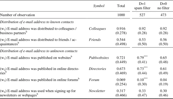
Central Costs ... B.31 Spam-induced Working Time Losses ... B.31 Individual Factors ... B.32 Reactance ... B.33 Distribution of e-mail addresses ... B.34 Estimation Results of the Logit Model ... B.35 Matching Results ... B.36 Group Analysis: Matching Results (group-specific scores) ... B.36 Sensitivity Analysis, Unobserved Heterogeneity ... B.37

Abschnitt C

Services für Messeaussteller und -besucher ... C.6

Praxisbeispiele - Entscheidungsalternativen ... C.10

Formen der Spezifität ... C.13

Hypothesen zu Einflussfaktoren des Transaktionskostenansatzes ... C.14

Weitere Einflussfaktoren ... C.15

Gastronomie-Services ... C.18

Standbau-Services ... C.20

Abkürzungsverzeichnis

ACM Association for Computing Machinery

ATE Average treatment effect

ATT Averate treatment effect of the treated ATU Averate treatment effect of the untreated Aufl. Auflage

AUMA Ausstellungs- und Messe-Ausschuss der Deutschen Wirtschaft e.V.

biasaft Standardized bias after matching biasbef Standardized bias before matching bzw. beziehungsweise

CIA Conditional independence assumption

Coef. Coefficient Const. Constant

CS Common support

CVM Covariate matching

DBW Die Betriebswirtschaft (Zeitschrift)

d. h. das heißt

DID Difference-in-differences DMTP Differentiated mail transfer protocol

eds Editors

e. g. for example

E-mail Electronic mail

Est. Estimator

et al. et alii (und andere)

etc. et cetera

e. V. eingetragener Verein

FAMAB Verband Direkte Wirtschaftskommunikation e.V.

Hrsg. Herausgeber

IFAU Institute for Labour Market Policy Evaluation IIA Independence for irrelevant alternatives assumption

IS Information systems

ISMA International Securities Market Association ISP Internet service provider

ISR Information Systems Research (Zeitschrift)

IT Information technology

IZA Forschungsinstitut zur Zukunft der Arbeit

Jg. Jahrgang

KM Kernel matching

LLM Local linear matching

LPM Local polynomial matching

MoB Make-or-buy NCDS National child development study

NN Nearest neighbour

No. Number Nr. Nummer

NSW National supported work demonstration Obs. Observations

OECD Organisation for Economic Cooperation and Development

offsup Off support

OLS Ordinary least squares regression pp pages

PS Propensity score

PSM Propensity score matching

S. Seite

SATT Sample average treatment effect of the treated

SB Standardized bias

s.e. Standard error

SIAW Schweizerisches Institut für Angewandte Wirtschaftsforschung SPAM Unsolicited bulk messages with commercial content

SUTVA Stable unit treatment value assumption

u. a. und andere

UI Unemployment insurance

vgl. vergleiche

Vol. Volume

WiSt Wirtschaftswissenschaftliches Studium (Zeitschrift)

www World wide web

z. B. zum Beispiel

ZEW Zentrum Europäische Wirtschaftsforschung GmbH

ZfbF Schmalenbachs Zeitschrift für betriebswirtschaftliche Forschung

Symbolverzeichnis

β Coefficient of observable covariates X

b(X) Balancing score

CI+ Upper bound confidence interval CI- Lower bound confidence interval

D Treatment indicator

E[(.)] Expectation operator

f ˆ (.) Nonparametric densitiy estimator

γ Coefficient of unobservable covariates U

k Number of continuous covariates

K

_M

(i) Number of times individual i is used as a match

1

λ

0

Mean of Y(1) for individuals outside common support L Number of options (treatments), with l=1,…,m,…,L

M Number of matches

N Set of individuals, with i=1,…,N

p Polynomial order

P(.) Probability operator

Pr(.) Probability operator

P(X) Propensity Score

P Sample proportion of persons taking treatment

q Treshold amount

σ

²1(0)

Conditional outcome variance

)

ˆ

( q

S

P

Region of common support (given a treshold amount q) Sig+ Upper bound significance level

Sig- Lower bound significance level

t-hat+ Upper bound Hodges-Lehmann point estimate t-hat- Lower bound Hodges-Lehmann point estimate

τ

i

Individual treatment effect

τ

ATE

Average treatment effect

τ

ATT

Average treatment effect of the treated

τ

SATT

Sample average treatment effect of the treated

t Posttreatment period

t’ Pretreatment period

U Unobservable covariates

Var

ATE

Variance bound for ATE Var

ATT

Variance bound for ATT

Var

SATT

Variance of sample average treatement effect Var( τ ˆ

_ATT

) Variance approximation by Lechner

V

1[0]

(X) Variance of X in the treatment [control] group before matching V

_1M[0M]

(X) Variance of X in the treatment [control] group after matching

w(.) Weighting function

X Observable covariates

X

1[1M]

Sample average of X in the treatment group before [after] matching X

_0[0M]

Sample average of X in the control group before [after] matching

Y Outcome variable

Y(D) Potential outcome given D

Ω Set of the population of interest

Überblick

Die vorliegende kumulative Dissertation untersucht zwei ausgewählte Problembereiche der Marketingforschung. Zum einen steht in den Abschnitten A und B die Selbstselektions- problematik im Fokus. Werden in einem nicht-experimentellen Umfeld kausale Maßnahmen- effekte ermittelt, können Selbstselektionsverzerrungen auftreten, da eine Zuordnung zur Maß- nahme nicht zufällig - wie etwa in einem experimentellen Umfeld

¹

- erfolgt. In Abschnitt A wird eine Analysemethode im Detail erläutert, die dem Problem der Selbstselektion Rechnung trägt. In Abschnitt B wird ein Anwendungsbeispiel für diese Methode präsentiert. Zum ande- ren wird in Abschnitt C eine Make-or-Buy-Fragestellung qualitativ analysiert. Dabei wird der Frage nachgegangen, ob es für ein Unternehmen profitabler ist, Produkte oder Dienstleistun- gen selbst zu fertigen bzw. zu erbringen (Make) oder auf dem Markt zu beschaffen (Buy).

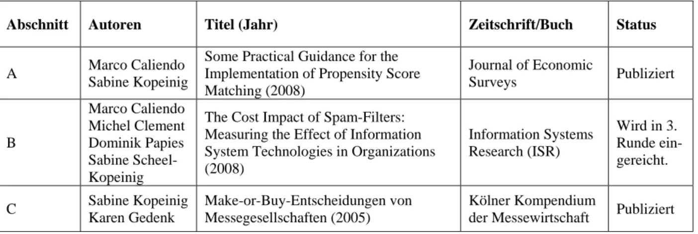
In den nachfolgenden Abschnitten A bis C werden die dieser Arbeit zugrundeliegenden drei Artikel präsentiert. Die nachstehende Tabelle fasst diese Artikel zusammen:

Abschnitt Autoren Titel (Jahr) Zeitschrift/Buch Status

A Marco Caliendo

Sabine Kopeinig

Some Practical Guidance for the Implementation of Propensity Score Matching (2008)

Journal of Economic

Surveys Publiziert

B

Marco Caliendo Michel Clement Dominik Papies Sabine Scheel- Kopeinig

The Cost Impact of Spam-Filters:

Measuring the Effect of Information System Technologies in Organizations (2008)

Information Systems Research (ISR)

Wird in 3.

Runde ein- gereicht.

C Sabine Kopeinig Karen Gedenk

Make-or-Buy-Entscheidungen von Messegesellschaften (2005)

Kölner Kompendium

der Messewirtschaft Publiziert

Tabelle 1: Übersicht der Artikel

Die Artikel der Abschnitte A Caliendo und Kopeinig (2008) sowie C Kopeinig und Gedenk (2005) sind in der vorliegenden Form im Journal of Economic Surveys bzw. Kölner Kompen- dium der Messewirtschaft publiziert. Der Artikel aus Abschnitt B Caliendo/Clement/Papies und Scheel-Kopeinig (2008) ist als IZA Discussion Paper veröffentlicht. Dieser Artikel befin- det sich im „editorial process“ und wird in dritter Runde bei der Zeitschrift Information Sys- tems Research (ISR) eingereicht. Im folgenden Überblick erfolgt eine kurze Zusammen-

1 Vgl. Harrison, G. W./List, J. A. (2004).

fassung der zentralen Erkenntnisse der oben genannten Artikel unter Darlegung der verfolgten Zielsetzung und der verwendeten Vorgehensweise.

Die Arbeiten in den Abschnitten A und B behandeln die Selbstselektionsproblematik. Dabei wird in Caliendo und Kopeinig (2008) eine Analysemethode - Propensity Score Matching (PSM) - im Detail vorgestellt. In Caliendo/Clement/Papies und Scheel-Kopeinig (2008) wird ein Anwendungsbeispiel für diese Methode präsentiert. In der empirischen Marketing- forschung sollen häufig Erfolgswirkungen von Marketingmaßnahmen ermittelt werden. Nicht immer sind experimentelle Untersuchungsdesigns möglich, um kausale Effekte dieser Maß- nahmen zu schätzen. Sollen beispielsweise Bonusprogramme oder Messebeteiligungen eva- luiert werden, muss häufig auf nicht-experimentelle Daten zurückgegriffen werden. Das inhä- rente Problem der Selbstselektion soll an dem nachfolgenden Beispiel verdeutlicht werden:

Wird der Effekt einer Messeteilnahme lediglich dadurch ermittelt, dass ein Zielgrößenver- gleich (z. B. Auftragsvolumen) zwischen Messeausstellern und Nichtausstellern erfolgt, dann wird vernachlässigt, dass unter Umständen gerade erfolgreichere Unternehmen an der Messe teilnehmen und sich so also „selbst zur Maßnahme selektieren“. Dabei kann die Entscheidung an der Messe teilzunehmen sowohl von beobachtbaren (z. B. Exportvolumen, Mitarbeiterzahl der Unternehmen etc.) als auch von unbeobachtbaren Eigenschaften der Unternehmen abhän- gen. Die zentrale Idee des PSM-Ansatzes

²

ist es, aus der Gruppe der Nichtteilnehmer nur jene Untersuchungseinheiten für den Zielgrößenvergleich heranzuziehen, die den Teilnehmern bezüglich beobachtbarer Eigenschaften am ähnlichsten sind. Unterschiede in der Zielgröße zwischen den Teilnehmern an einer Maßnahme und der adjustierten Kontrollgruppe können dann als Maßnahmeneffekt interpretiert werden.

³

Soll ein Maßnahmeneffekt mit Hilfe des Propensity Score Matchings evaluiert werden, ist der Anwender mit einer Vielzahl an Implementierungsschritten und Detailfragen konfrontiert. In methodischen Standardwerken

⁴

wird PSM noch nicht besprochen. Daher wird in Caliendo

2 Propensity Score Matching geht zentral auf die Arbeiten von Rubin, D. (1974) sowie Rosenbaum, P./Rubin, D.

(1983b, 1985) zurück.

3 Zentrale Annahme des Matching-Ansatzes ist, dass Unterschiede zwischen Teilnehmern und Nichtteilnehmern lediglich auf beobachtbaren Eigenschaften beruhen. Diese Annahme ist u. a. als „selection on observables“ be- kannt; vgl. Heckman, J./Robb, R. (1985).

4 Z. B. Backhaus, K./Erichson, B./Plinke, W./Weiber, R. (2008) oder Greene, W. H. (2003).

und Kopeinig (2008) dem PSM-Anwender ein Leitfaden für die Umsetzung der Implemen- tierungsschritte und der damit verbundenen Entscheidungen an die Hand gegeben werden.

Nach einer Darstellung des formalen Rahmens wird im Beitrag A gezeigt, wie PSM das Selbstselektionsproblem lösen kann und welche zentralen Annahmen dazu nötig sind.

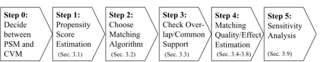
⁵

Es werden fünf zentrale Implementierungsschritte aufgezeigt und mögliche Entscheidungs- alternativen ausführlich diskutiert. Bei den Implementierungsschritten handelt es sich um die Schätzung des Propensity Scores (Schritt 1), die Auswahl des Matching-Algorithmus ( Schritt 2), Overlap und Common Support (Schritt 3), Matching Qualität und Schätzung des Maßnahmeneffektes (Schritt 4) sowie um Sensitivitätsanalysen (Schritt 5). Abschließend werden noch praxisrelevante Sachverhalte - mit welchen PSM-Anwender konfrontiert sein können - dargestellt und Weiterentwicklungen des PSM-Ansatzes diskutiert.

Im Ergebnis liefert der vorliegende Beitrag eine bis dato einmalige, anwendungsorientierte, sequenzielle und gut verständliche Orientierungs- und Entscheidungshilfe bei der PSM- Implementierung. Außerdem erfolgt eine umfassende Bündelung und Auswertung der wissen- schaftlichen Literatur zum Thema „Propensity Score Matching“.

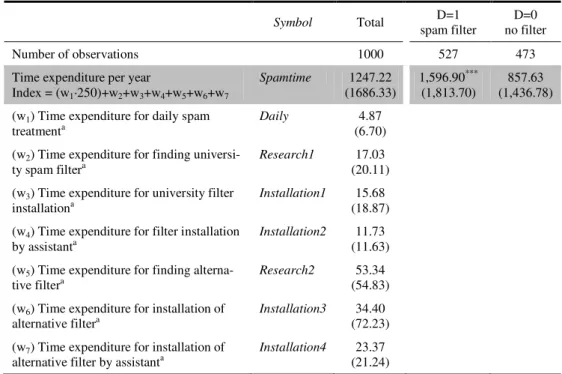
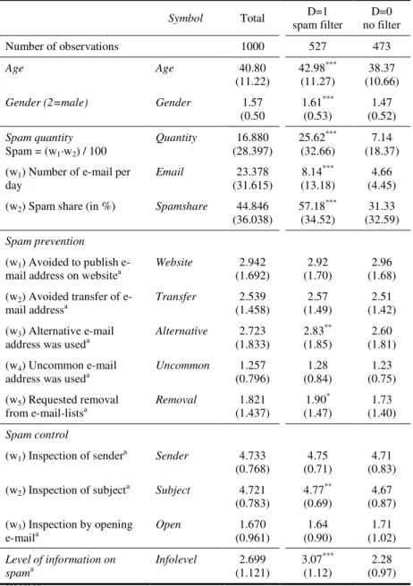
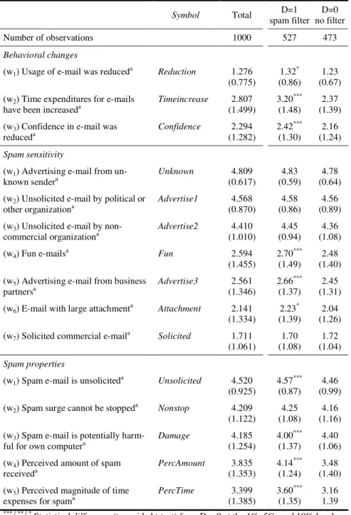
Im Beitrag B Caliendo/Clement/Papies und Scheel-Kopeinig (2008) wird analysiert, ob die Installation eines Spam-Filters die Arbeitszeitverluste von Mitarbeitern, die u. a. dadurch ent- stehen, dass Spam-Mails überprüft werden müssen, reduzieren kann. Um diesen Maßnahmen- effekt mit nicht-experimentellen Daten unter Berücksichtigung möglicher Selbstselektions- verzerrungen zu messen, wird das Verfahren des Propensity Score Matchings angewandt.

Im Zusammenhang mit Spam-Mails entstehen Unternehmen sowohl zentrale Kosten auf IT- Ebene als auch individuelle Kosten auf Mitarbeiterebene. Sowohl eine Quantifizierung dieser Kosten als auch eine Analyse der Kostenwirkungen einer Schutzmaßnahme gegen Spam (Spam-Filter) erfolgte in der wissenschaftlichen Literatur bislang noch nicht. Der vorliegende Beitrag versucht diese Forschungslücke zu schließen.

5 Vgl. dazu z. B. Heckman, J./Ichimura, H./Todd, P. (1997a).

Nach einer Zusammenfassung der bisherigen „Spam-Forschung“ und einer kurzen Beschrei- bung der Methode des Propensity Score Matchings wird die Datenerhebung und das For- schungsdesign beschrieben und deskriptive Ergebnisse präsentiert. Im Anschluss folgt die Matchinganalyse. Nach einer Darstellung der Matchingergebnisse werden auch Sensitivitäts- analysen hinsichtlich Effektheterogentität und unbeobachtbarer Heterogentität durchgeführt.

Der vorliegende Beitrag zeigt, dass Spam-Mails durchaus nennenswerte Kosten auf indivi- dueller Mitarbeiterebene aber vernachlässigbare Kosten auf IT-Ebene verursachen. Die Instal- lation eines Spam Filters kann die Arbeitszeitverluste, die Mitarbeitern durch die Kontrolle und das Löschen von Spam Mails entstehen, um ca. 35 % reduzieren. Die Effektivität der Schutzmaßnahme hängt aber im Einzelnen maßgeblich von der individuellen Anzahl der er- haltenen Spam-Mails und vom Spam-Kenntnisstand des Mitarbeiters ab.

Kopeinig und Gedenk (2005) untersuchen im Messe-Kontext die Vorteilhaftigkeit von Make- or-Buy-(MoB)-Entscheidungen für Messe-Dienstleistungen, wie Gastronomie- oder Stand- bau-Services. Ziel des Beitrags ist es, Messeunternehmen eine Entscheidungshilfe bei der Auswahl von möglichen Make-or-Buy-Alternativen an die Hand zu geben. Nach einer Syste- matisierung relevanter MoB-Entscheidungen von Messegesellschaften werden mögliche MoB-Entscheidungsalternativen dargestellt. Dabei gibt es zwischen den beiden Extrema

„Make“ und „Buy“ eine Vielzahl relevanter Organisationsformen, bei denen Messe- gesellschaften mit anderen Unternehmen kooperieren (Cooperate).

⁶

In der Praxis können über Messegesellschaften und Messe-Dienstleistungen hinweg die gewählten Organisationsformen erheblich variieren. Beispielsweise werden am Messestandort Frankfurt am Main Gastrono- mie-Services über ein Tochterunternehmen selbst erbracht. Andere Messegesellschaften favo- risieren eine marktnahe Alternative und schließen Pachtverträge mit unabhängigen Messe- gastronomen ab.

Im Beitrag werden Einflussfaktoren auf die Vorteilhaftigkeit der Handlungsalternativen

„Make“ vs. „Buy“ herausgearbeitet. Diese werden zum einen aus dem Transaktionskosten- ansatz

⁷

und zum anderen aus der konzeptionellen Literatur zum Messewesen abgeleitet. Im

6 Vgl. Picot, A. (1991).

7 Vgl. Coase, R. H. (1937), Williamson, O. E. (1975, 1985).

speziellen erfolgt eine qualitative Analyse der Vorteilhaftigkeit von „Make“-vs.“Buy“- Entscheidungen für zwei exemplarische Messe-Dienstleistungen.

Im Ergebnis bietet der vorliegende Beitrag speziell Messeunternehmen eine Entscheidungs-

hilfe für den Entscheidungsprozess „Make-vs.-Buy“ für einzelne Messedienstleistungen. Die

im Fokus der Arbeit stehende Vorgehensweise der Vorteilhaftigkeitsanalyse kann allgemein

auf Make-or-Buy-Fragestellungen in anderen Branchen übertragen werden.

Abschnitt A:

Caliendo, Marco/Kopeinig, Sabine: Some Practical Guidance for the Implementation of Propensity Score Matching

Caliendo, Marco/Kopeinig, Sabine: Some Practical Guidance for the Implementation of

Propensity Score Matching, Journal of Economic Surveys, 22. Jg. (1), 2008, S. 31 - 72.

SOME PRACTICAL GUIDANCE FOR THE IMPLEMENTATION OF PROPENSITY

SCORE MATCHING

Marco Caliendo IZA, Bonn

Sabine Kopeinig University of Cologne

Abstract. Propensity score matching (PSM) has become a popular approach to estimate causal treatment effects. It is widely applied when evaluating labour market policies, but empirical examples can be found in very diverse fields of study. Once the researcher has decided to use PSM, he is confronted with a lot of questions regarding its implementation. To begin with, a first decision has to be made concerning the estimation of the propensity score. Following that one has to decide which matching algorithm to choose and determine the region of common support. Subsequently, the matching quality has to be assessed and treatment effects and their standard errors have to be estimated. Furthermore, questions like

‘what to do if there is choice-based sampling?’ or ‘when to measure effects?’

can be important in empirical studies. Finally, one might also want to test the sensitivity of estimated treatment effects with respect to unobserved heterogeneity or failure of the common support condition. Each implementation step involves a lot of decisions and different approaches can be thought of. The aim of this paper is to discuss these implementation issues and give some guidance to researchers who want to use PSM for evaluation purposes.

Keywords. Propensity score matching; Treatment effects; Evaluation; Sensitivity analysis; Implementation

1. Introduction

Matching has become a popular approach to estimate causal treatment effects. It is widely applied when evaluating labour market policies (see e.g., Heckman et al., 1997a; Dehejia and Wahba, 1999), but empirical examples can be found in very diverse fields of study. It applies for all situations where one has a treatment, a group of treated individuals and a group of untreated individuals. The nature of treatment may be very diverse. For example, Perkinset al.(2000) discuss the usage of matching in pharmacoepidemiologic research. Hitt and Frei (2002) analyse the effect of online banking on the profitability of customers. Davies and Kim (2003) compare

Journal of Economic Surveys(2008) Vol. 22, No. 1, pp. 31–72

the effect on the percentage bid–ask spread of Canadian firms being interlisted on a US Exchange, whereas Brand and Halaby (2006) analyse the effect of elite college attendance on career outcomes. Ham et al. (2004) study the effect of a migration decision on the wage growth of young men and Bryson (2002) analyses the effect of union membership on wages of employees. Every microeconometric evaluation study has to overcome the fundamental evaluation problem and address the possible occurrence of selection bias. The first problem arises because we would like to know the difference between the participants’ outcome with and without treatment. Clearly, we cannot observe both outcomes for the same individual at the same time. Taking the mean outcome of nonparticipants as an approximation is not advisable, since participants and nonparticipants usually differ even in the absence of treatment.

This problem is known as selection bias and a good example is the case where high-skilled individuals have a higher probability of entering a training programme and also have a higher probability of finding a job. The matching approach is one possible solution to the selection problem. It originated from the statistical literature and shows a close link to the experimental context.¹ Its basic idea is to find in a large group of nonparticipants those individuals who are similar to the participants in all relevant pretreatment characteristicsX. That being done, differences in outcomes of this well selected and thus adequate control group and of participants can be attributed to the programme. The underlying identifying assumption is known as unconfoundedness, selection on observables or conditional independence. It should be clear that matching is no ‘magic bullet’ that will solve the evaluation problem in any case. It should only be applied if the underlying identifying assumption can be credibly invoked based on the informational richness of the data and a detailed understanding of the institutional set-up by which selection into treatment takes place (see for example the discussion in Blundellet al., 2005). For the rest of the paper we will assume that this assumption holds.

Since conditioning on all relevant covariates is limited in the case of a high dimensional vector X (‘curse of dimensionality’), Rosenbaum and Rubin (1983b) suggest the use of so-called balancing scores b(X), i.e. functions of the relevant observed covariates X such that the conditional distribution of X given b(X) is independent of assignment into treatment. One possible balancing score is the propensity score, i.e. the probability of participating in a programme given observed characteristics X. Matching procedures based on this balancing score are known as propensity score matching (PSM) and will be the focus of this paper. Once the researcher has decided to use PSM, he is confronted with a lot of questions regarding its implementation. Figure 1 summarizes the necessary steps when implementing PSM.²

The aim of this paper is to discuss these issues and give some practical guidance to researchers who want to use PSM for evaluation purposes. The paper is organized as follows. In Section 2, we will describe the basic evaluation framework and possible treatment effects of interest. Furthermore we show how PSM solves the evaluation problem and highlight the implicit identifying assumptions. In Section 3, we will focus on implementation steps of PSM estimators. To begin with, a first decision has to be made concerning the estimation of the propensity score

Step 0:

Decide between PSM and CVM

Step 1:

Propensity Score Estimation

(Sec. 3.1)

Step 2:

Choose Matching Algorithm

(Sec. 3.2)

Step 3:

Check Over- lap/Common Support

(Sec. 3.3)

Step 5:

Sensitivity Analysis

(Sec. 3.9)

Step 4:

Matching Quality/Effect Estimation

(Sec. 3.4-3.8)

Figure 1. PSM – Implementation Steps.

(see Section 3.1). One has not only to decide about the probability model to be used for estimation, but also about variables which should be included in this model. In Section 3.2, we briefly evaluate the (dis-)advantages of different matching algorithms. Following that we discuss how to check the overlap between treatment and comparison group and how to implement the common support requirement in Section 3.3. In Section 3.4 we will show how to assess the matching quality. Subsequently we present the problem of choice-based sampling and discuss the question ‘when to measure programme effects?’ in Sections 3.5 and 3.6.

Estimating standard errors for treatment effects will be discussed in Section 3.7 before we show in 3.8 how PSM can be combined with other evaluation methods. The following Section 3.9 is concerned with sensitivity issues, where we first describe approaches that allow researchers to determine the sensitivity of estimated effects with respect to a failure of the underlying unconfoundedness assumption. After that we introduce an approach that incorporates information from those individuals who failed the common support restriction, to calculate bounds of the parameter of interest, if all individuals from the sample at hand would have been included.

Section 3.10 will briefly discuss the issues of programme heterogeneity, dynamic selection problems, and the choice of an appropriate control group and includes also a brief review of the available software to implement matching. Finally, Section 4 reviews all steps and concludes.

2. Evaluation Framework and Matching Basics

Roy–Rubin Model

Inference about the impact of a treatment on the outcome of an individual involves speculation about how this individual would have performed had (s)he not received the treatment. The standard framework in evaluation analysis to formalize this problem is the potential outcome approach or Roy–Rubin model (Roy, 1951; Rubin, 1974). The main pillars of this model are individuals, treatment and potential outcomes. In the case of a binary treatment the treatment indicator D_iequals one if individualireceives treatment and zero otherwise. The potential outcomes are then defined asY_i(D_i) for each individuali, wherei =1,. . .,N andNdenotes the total population. The treatment effect for an individual ican be written as

τ_i =Y_i(1)−Y_i(0) (1)

The fundamental evaluation problem arises because only one of the potential outcomes is observed for each individuali. The unobserved outcome is called the counterfactual outcome. Hence, estimating the individual treatment effectτ_i is not possible and one has to concentrate on (population) average treatment effects.³

Parameter of Interest and Selection Bias

Two parameters are most frequently estimated in the literature. The first one is the population average treatment effect (ATE), which is simply the difference of the expected outcomes after participation and nonparticipation:

τ_ATE=E(τ)=E[Y(1)−Y(0)] (2) This parameter answers the question: ‘What is the expected effect on the outcome if individuals in the population were randomly assigned to treatment?’ Heckman (1997) notes that this estimate might not be of relevance to policy makers because it includes the effect on persons for whom the programme was never intended. For example, if a programme is specifically targeted at individuals with low family income, there is little interest in the effect of such a programme for a millionaire. Therefore, the most prominent evaluation parameter is the so-called average treatment effect on the treated (ATT), which focuses explicitly on the effects on those for whom the programme is actually intended. It is given by

τATT =E(τ|D=1)=E[Y(1)|D=1]−E[Y(0)|D=1] (3) The expected value of ATT is defined as the difference between expected outcome values with and without treatment for those who actually participated in treatment.

In the sense that this parameter focuses directly on actual treatment participants, it determines the realized gross gain from the programme and can be compared with its costs, helping to decide whether the programme is successful or not (Heckmanet al., 1999). The most interesting parameter to estimate depends on the specific evaluation context and the specific question asked. Heckman et al. (1999) discuss further parameters, like the proportion of participants who benefit from the programme or the distribution of gains at selected base state values. For most evaluation studies, however, the focus lies on ATT and therefore we will focus on this parameter, too.⁴ As the counterfactual mean for those being treated – E[Y(0)|D =1] – is not observed, one has to choose a proper substitute for it in order to estimate ATT. Using the mean outcome of untreated individuals E[Y(0)|D = 0] is in nonexperimental studies usually not a good idea, because it is most likely that components which determine the treatment decision also determine the outcome variable of interest.

Thus, the outcomes of individuals from the treatment and comparison groups would differ even in the absence of treatment leading to a ‘selection bias’. For ATT it can be noted as

E[Y(1)|D=1]−E[Y(0)|D=0]=τ_{AT T} +E[Y(0)|D=1]−E[Y(0)|D=0] (4)

The difference between the left-hand side of equation (4) andτ_ATT is the so-called

‘selection bias’. The true parameterτ_ATT is only identified if

E[Y(0)|D=1]−E[Y(0)|D=0]=0 (5) In social experiments where assignment to treatment is random this is ensured and the treatment effect is identified.⁵In nonexperimental studies one has to invoke some identifying assumptions to solve the selection problem stated in equation (4).

Unconfoundedness and Common Support

One major strand of evaluation literature focuses on the estimation of treatment effects under the assumption that the treatment satisfies some form of exogene- ity. Different versions of this assumption are referred to as unconfoundedness (Rosenbaum and Rubin, 1983b), selection on observables (Heckman and Robb, 1985) or conditional independence assumption (CIA) (Lechner, 1999). We will use these terms throughout the paper interchangeably. This assumption implies that systematic differences in outcomes between treated and comparison individuals with the same values for covariates are attributable to treatment. Imbens (2004) gives an extensive overview of estimating ATEs under unconfoundedness. The identifying assumption can be written as

Assumption 1.Unconfoundedness: Y(0),Y(1) D | X

where denotes independence, i.e. given a set of observable covariates X which are not affected by treatment, potential outcomes are independent of treatment assignment. This implies that all variables that influence treatment assignment and potential outcomes simultaneously have to be observed by the researcher. Clearly, this is a strong assumption and has to be justified by the data quality at hand. For the rest of the paper we will assume that this condition holds. If the researcher believes that the available data are not rich enough to justify this assumption, he has to rely on different identification strategies which explicitly allow selection on unobservables, too. Prominent examples are difference-in-differences (DID) and instrumental variables estimators.⁶We will show in Section 3.8 how propensity score matching can be combined with some of these methods.

A further requirement besides independence is the common support or overlap condition. It rules out the phenomenon of perfect predictability ofDgivenX.

Assumption 2.Overlap:0< P(D =1|X)<1.

It ensures that persons with the same X values have a positive probability of being both participants and nonparticipants (Heckmanet al., 1999). Rosenbaum and Rubin (1983b) call Assumptions 1 and 2 together ‘strong ignorability’. Under ‘strong ignorability’ ATE in (2) and ATT in (3) can be defined for all values ofX. Heckman et al.(1998b) demonstrate that the ignorability or unconfoundedness conditions are overly strong. All that is needed for estimation of (2) and (3) is mean independence.

However, Lechner (2002) argues that Assumption 1 has the virtue of identifying

mean effects for all transformations of the outcome variables. The reason is that the weaker assumption of mean independence is intrinsically tied to functional form assumptions, making an identification of average effects on transformations of the original outcome impossible (Imbens, 2004). Furthermore, it will be difficult to argue why conditional mean independence should hold and Assumption 1 might still be violated in empirical studies.

If we are interested in estimating the ATT only, we can weaken the unconfound- edness assumption in a different direction. In that case one needs only to assume Assumption 3.Unconfoundedness for controls: Y(0) D| X

and the weaker overlap assumption

Assumption 4.Weak overlap: P(D =1| X)<1.

These assumptions are sufficient for identification of (3), because the moments of the distribution ofY(1) for the treated are directly estimable.

Unconfoundedness given the Propensity Score

It should also be clear that conditioning on all relevant covariates is limited in the case of a high dimensional vector X. For instance if X contains s covariates which are all dichotomous, the number of possible matches will be 2^s. To deal with this dimensionality problem, Rosenbaum and Rubin (1983b) suggest using so-called balancing scores. They show that if potential outcomes are independent of treatment conditional on covariates X, they are also independent of treatment conditional on a balancing score b(X). The propensity score P(D = 1 | X) = P(X), i.e. the probability for an individual to participate in a treatment given his observed covariates X, is one possible balancing score. Hence, if Assumption 1 holds, all biases due to observable components can be removed by conditioning on the propensity score (Imbens, 2004).

Corollary 1.Unconfoundedness given the propensity score: Y(0),Y(1)D|P(X).⁷ Estimation Strategy

Given that CIA holds and assuming additionally that there is overlap between both groups, the PSM estimator for ATT can be written in general as

τ_{AT T}^{P S M} =E_P(X)|D=1{E[Y(1)|D=1,P(X)]−E[Y(0)|D=0,P(X)]} (6) To put it in words, the PSM estimator is simply the mean difference in outcomes over the common support, appropriately weighted by the propensity score distribution of participants. Based on this brief outline of the matching estimator in the general evaluation framework, we are now going to discuss the implementation of PSM in detail.

3. Implementation of Propensity Score Matching 3.1 Estimating the Propensity Score

When estimating the propensity score, two choices have to be made. The first one concerns the model to be used for the estimation, and the second one the variables to be included in this model. We will start with the model choice before we discuss which variables to include in the model.

Model Choice – Binary Treatment

Little advice is available regarding which functional form to use (see for example the discussion in Smith, 1997). In principle any discrete choice model can be used.

Preference for logit or probit models (compared to linear probability models) derives from the well-known shortcomings of the linear probability model, especially the unlikeliness of the functional form when the response variable is highly skewed and predictions that are outside the [0, 1] bounds of probabilities. However, when the purpose of a model is classification rather than estimation of structural coefficients, it is less clear that these criticisms apply (Smith, 1997). For the binary treatment case, where we estimate the probability of participation versus nonparticipation, logit and probit models usually yield similar results. Hence, the choice is not too critical, even though the logit distribution has more density mass in the bounds.

Model Choice – Multiple Treatments

However, when leaving the binary treatment case, the choice of the model becomes more important. The multiple treatment case (as discussed in Imbens (2000) and Lechner (2001a)) consists of more than two alternatives, for example when an individual is faced with the choice to participate in job-creation schemes, vocational training or wage subsidy programmes or to not participate at all (we will describe this approach in more detail in Section 3.10). For that case it is well known that the multinomial logit is based on stronger assumptions than the multinomial probit model, making the latter the preferable option.⁸ However, since the multinomial probit is computationally more burdensome, a practical alternative is to estimate a series of binomial models as suggested by Lechner (2001a). Bryson et al.(2002) note that there are two shortcomings regarding this approach. First, as the number of options increases, the number of models to be estimated increases disproportionately (for L options we need 0.5(L(L − 1)) models). Second, in each model only two options at a time are considered and consequently the choice is conditional on being in one of the two selected groups. On the other hand, Lechner (2001a) compares the performance of the multinomial probit approach and series estimation and finds little difference in their relative performance. He suggests that the latter approach may be more robust since a mis-specification in one of the series will not compromise all others as would be the case in the multinomial probit model.

Variable Choice:

More advice is available regarding the inclusion (or exclusion) of covariates in the propensity score model. The matching strategy builds on the CIA, requiring that the outcome variable(s) must be independent of treatment conditional on the propensity score. Hence, implementing matching requires choosing a set of variables Xthat credibly satisfy this condition. Heckmanet al.(1997a) and Dehejia and Wahba (1999) show that omitting important variables can seriously increase bias in resulting estimates. Only variables that influence simultaneously the participation decision and the outcome variable should be included. Hence, economic theory, a sound knowledge of previous research and also information about the institutional settings should guide the researcher in building up the model (see e.g., Sianesi, 2004; Smith and Todd, 2005). It should also be clear that only variables that are unaffected by participation (or the anticipation of it) should be included in the model. To ensure this, variables should either be fixed over time or measured before participation. In the latter case, it must be guaranteed that the variable has not been influenced by the anticipation of participation. Heckmanet al.(1999) also point out that the data for participants and nonparticipants should stem from the same sources (e.g. the same questionnaire). The better and more informative the data are, the easier it is to credibly justify the CIA and the matching procedure. However, it should also be clear that ‘too good’ data is not helpful either. If P(X)=0 or P(X)=1 for some values ofX, then we cannot use matching conditional on thoseX values to estimate a treatment effect, because persons with such characteristics either always or never receive treatment. Hence, the common support condition as stated in Assumption 2 fails and matches cannot be performed. Some randomness is needed that guarantees that persons with identical characteristics can be observed in both states (Heckman et al., 1998b).

In cases of uncertainty of the proper specification, sometimes the question may arise whether it is better to include too many rather than too few variables. Bryson et al.(2002) note that there are two reasons why over-parameterized models should be avoided. First, it may be the case that including extraneous variables in the participation model exacerbates the support problem. Second, although the inclusion of nonsignificant variables in the propensity score specification will not bias the propensity score estimates or make them inconsistent, it can increase their variance.

The results from Augurzky and Schmidt (2001) point in the same direction.

They run a simulation study to investigate PSM when selection into treatment is remarkably strong, and treated and untreated individuals differ considerably in their observable characteristics. In their set-up, explanatory variables in the selection equation are partitioned into three sets. The first set (set 1) includes covariates which strongly influence the treatment decision but weakly influence the outcome variable. Furthermore, they include covariates which are relevant to the outcome but irrelevant to the treatment decision (set 2) and covariates which influence both (set 3). Including the full set of covariates in the propensity score specification (full model including all three sets of covariates) might cause problems in small samples in terms of higher variance, since either some treated have to be discarded from the

analysis or control units have to be used more than once. They show that matching on an inconsistent estimate of the propensity score (i.e. partial model including only set 3 or both sets 1 and 3) produces better estimation results of the ATE.

On the other hand, Rubin and Thomas (1996) recommend against ‘trimming’

models in the name of parsimony. They argue that a variable should only be excluded from analysis if there is consensus that the variable is either unrelated to the outcome or not a proper covariate. If there are doubts about these two points, they explicitly advise to include the relevant variables in the propensity score estimation.

By these criteria, there are both reasons for and against including all of the reasonable covariates available. Basically, the points made so far imply that the choice of variables should be based on economic theory and previous empirical findings. But clearly, there are also some formal (statistical) tests which can be used. Heckman et al. (1998a), Heckman and Smith (1999) and Black and Smith (2004) discuss three strategies for the selection of variables to be used in estimating the propensity score.

Hit or Miss Method

The first one is the ‘hit or miss’ method or prediction rate metric, where variables are chosen to maximize the within-sample correct prediction rates. This method classifies an observation as ‘1’ if the estimated propensity score is larger than the sample proportion of persons taking treatment, i.e. ˆP(X)> P. If ˆP(X)≤ P observations are classified as ‘0’. This method maximizes the overall classification rate for the sample assuming that the costs for the misclassification are equal for the two groups (Heckmanet al., 1997a).⁹ But clearly, it has to be kept in mind that the main purpose of the propensity score estimation is not to predict selection into treatment as well as possible but to balance all covariates (Augurzky and Schmidt, 2001).

Statistical Significance

The second approach relies on statistical significance and is very common in textbook econometrics. To do so, one starts with a parsimonious specification of the model, e.g. a constant, the age and some regional information, and then ‘tests up’ by iteratively adding variables to the specification. A new variable is kept if it is statistically significant at conventional levels. If combined with the ‘hit or miss’ method, variables are kept if they are statistically significant and increase the prediction rates by a substantial amount (Heckmanet al., 1998a).

Leave-One-Out Cross-Validation

Leave-one-out cross-validation can also be used to choose the set of variables to be included in the propensity score. Black and Smith (2004) implement their model selection procedure by starting with a ‘minimal’ model containing only two variables. They subsequently add blocks of additional variables and compare the

resulting mean squared errors. As a note of caution, they stress that this amounts to choosing the propensity score model based on goodness-of-fit considerations, rather than based on theory and evidence about the set of variables related to the participation decision and the outcomes (Black and Smith, 2004). They also point out an interesting trade-off in finite samples between the plausibility of the CIA and the variance of the estimates. When using the full specification, bias arises from selecting a wide bandwidth in response to the weakness of the common support.

In contrast to that, when matching on the minimal specification, common support is not a problem but the plausibility of the CIA is. This trade-off also affects the estimated standard errors, which are smaller for the minimal specification where the common support condition poses no problem.

Finally, checking the matching quality can also help to determine the propensity score specification and we will discuss this point later in Section 3.4.

Overweighting some Variables

Let us assume for the moment that we have found a satisfactory specification of the model. It may sometimes be felt that some variables play a specifically important role in determining participation and outcome (Bryson et al., 2002). As an example, one can think of the influence of gender and region in determining the wage of individuals. Let us take as given for the moment that men earn more than women and the wage level is higher in region A compared to region B. If we add dummy variables for gender and region in the propensity score estimation, it is still possible that women in region B are matched with men in region A, since the gender and region dummies are only a subset of all available variables. There are basically two ways to put greater emphasis on specific variables. One can either find variables in the comparison group who are identical with respect to these variables, or carry out matching on subpopulations. The study from Lechner (2002) is a good example for the first approach. He evaluates the effects of active labour market policies in Switzerland and uses the propensity score as a ‘partial’ balancing score which is complemented by an exact matching on sex, duration of unemployment and native language. Heckman et al. (1997a, 1998a) use the second strategy and implement matching separately for four demographic groups. That implies that the complete matching procedure (estimating the propensity score, checking the common support, etc.) has to be implemented separately for each group. This is analogous to insisting on a perfect match, e.g. in terms of gender and region, and then carrying out propensity score matching. This procedure is especially recommendable if one expects the effects to be heterogeneous between certain groups.

Alternatives to the Propensity Score

Finally, it should also be noted that it is possible to match on a measure other than the propensity score, namely the underlying index of the score estimation.

The advantage of this is that the index differentiates more between observations in the extremes of the distribution of the propensity score (Lechner, 2000). This is

Matching Algorithms

Nearest Neighbour (NN)

Caliper and Radius

Stratification and Interval

Kernel and Local Linear

With/without replacement Oversampling (2-NN, 5-NN a.s.o.) Weights for oversampling

Max. tolerance level (caliper) 1-NN only or more (radius)

Number of strata/intervals

Kernel functions (e.g. Gaussian, a.s.o.) Bandwidth parameter

Figure 2. Different Matching Algorithms.

useful if there is some concentration of observations in the tails of the distribution.

Additionally, in some recent papers the propensity score is estimated by duration models. This is of particular interest if the ‘timing of events’ plays a crucial role (see e.g. Brodatyet al., 2001; Sianesi, 2004).

3.2 Choosing a Matching Algorithm

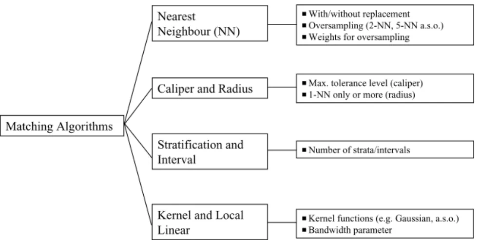
The PSM estimator in its general form was stated in equation (6). All matching estimators contrast the outcome of a treated individual with outcomes of comparison group members. PSM estimators differ not only in the way the neighbourhood for each treated individual is defined and the common support problem is handled, but also with respect to the weights assigned to these neighbours. Figure 2 depicts different PSM estimators and the inherent choices to be made when they are used.

We will not discuss the technical details of each estimator here at depth but rather present the general ideas and the involved trade-offs with each algorithm.¹⁰

Nearest Neighbour Matching

The most straightforward matching estimator is nearest neighbour (NN) matching.

The individual from the comparison group is chosen as a matching partner for a treated individual that is closest in terms of the propensity score. Several variants of NN matching are proposed, e.g. NN matching ‘with replacement’ and ‘without replacement’. In the former case, an untreated individual can be used more than once as a match, whereas in the latter case it is considered only once. Matching with replacement involves a trade-off between bias and variance. If we allow replacement, the average quality of matching will increase and the bias will decrease. This is of

particular interest with data where the propensity score distribution is very different in the treatment and the control group. For example, if we have a lot of treated individuals with high propensity scores but only few comparison individuals with high propensity scores, we get bad matches as some of the high-score participants will get matched to low-score nonparticipants. This can be overcome by allowing replacement, which in turn reduces the number of distinct nonparticipants used to construct the counterfactual outcome and thereby increases the variance of the estimator (Smith and Todd, 2005). A problem which is related to NN matching without replacement is that estimates depend on the order in which observations get matched. Hence, when using this approach it should be ensured that ordering is randomly done.¹¹

It is also suggested to use more than one NN (‘oversampling’). This form of matching involves a trade-off between variance and bias, too. It trades reduced variance, resulting from using more information to construct the counterfactual for each participant, with increased bias that results from on average poorer matches (see e.g. Smith, 1997). When using oversampling, one has to decide how many matching partners should be chosen for each treated individual and which weight (e.g. uniform or triangular weight) should be assigned to them.

Caliper and Radius Matching

NN matching faces the risk of bad matches if the closest neighbour is far away. This can be avoided by imposing a tolerance level on the maximum propensity score distance (caliper). Hence, caliper matching is one form of imposing a common support condition (we will come back to this point in Section 3.3). Bad matches are avoided and the matching quality rises. However, if fewer matches can be performed, the variance of the estimates increases.¹² Applying caliper matching means that an individual from the comparison group is chosen as a matching partner for a treated individual that lies within the caliper (‘propensity range’) and is closest in terms of propensity score. As Smith and Todd (2005) note, a possible drawback of caliper matching is that it is difficult to knowa priori what choice for the tolerance level is reasonable.

Dehejia and Wahba (2002) suggest a variant of caliper matching which is called radius matching. The basic idea of this variant is to use not only the NN within each caliper but all of the comparison members within the caliper. A benefit of this approach is that it uses only as many comparison units as are available within the caliper and therefore allows for usage of extra (fewer) units when good matches are (not) available. Hence, it shares the attractive feature of oversampling mentioned above, but avoids the risk of bad matches.

Stratification and Interval Matching

The idea of stratification matching is to partition the common support of the propensity score into a set of intervals (strata) and to calculate the impact within each interval by taking the mean difference in outcomes between treated and

control observations. This method is also known as interval matching, blocking and subclassification (Rosenbaum and Rubin, 1984). Clearly, one question to be answered is how many strata should be used in empirical analysis. Cochran (1968) shows that five subclasses are often enough to remove 95% of the bias associated with one single covariate. Since, as Imbens (2004) notes, all bias under unconfoundedness is associated with the propensity score, this suggests that under normality the use of five strata removes most of the bias associated with all covariates. One way to justify the choice of the number of strata is to check the balance of the propensity score (or the covariates) within each stratum (see e.g.

Aakvik, 2001). Most of the algorithms can be described in the following way.

First, check if within a stratum the propensity score is balanced. If not, strata are too large and need to be split. If, conditional on the propensity score being balanced, the covariates are unbalanced, the specification of the propensity score is not adequate and has to be respecified, e.g. through the addition of higher-order terms or interactions (see Dehejia and Wahba, 1999; Dehejia, 2005).

Kernel and Local Linear Matching

The matching algorithms discussed so far have in common that only a few observations from the comparison group are used to construct the counterfactual outcome of a treated individual. Kernel matching (KM) and local linear matching (LLM) are nonparametric matching estimators that use weighted averages of (nearly) all – depending on the choice of the kernel function – individuals in the control group to construct the counterfactual outcome. Thus, one major advantage of these approaches is the lower variance which is achieved because more information is used. A drawback of these methods is that possibly observations are used that are bad matches. Hence, the proper imposition of the common support condition is of major importance for KM and LLM. Heckmanet al. (1998b) derive the asymptotic distribution of these estimators and Heckmanet al.(1997a) present an application.

As Smith and Todd (2005) note, KM can be seen as a weighted regression of the counterfactual outcome on an intercept with weights given by the kernel weights.

Weights depend on the distance between each individual from the control group and the participant observation for which the counterfactual is estimated. It is worth noting that if weights from a symmetric, nonnegative, unimodal kernel are used, then the average places higher weight on persons close in terms of the propensity score of a treated individual and lower weight on more distant observations. The estimated intercept provides an estimate of the counterfactual mean. The difference between KM and LLM is that the latter includes in addition to the intercept a linear term in the propensity score of a treated individual. This is an advantage whenever comparison group observations are distributed asymmetrically around the treated observation, e.g. at boundary points, or when there are gaps in the propensity score distribution.

When applying KM one has to choose the kernel function and the bandwidth parameter. The first point appears to be relatively unimportant in practice (DiNardo and Tobias, 2001). What is seen as more important (see e.g. Silverman, 1986;

Pagan and Ullah, 1999) is the choice of the bandwidth parameter with the following

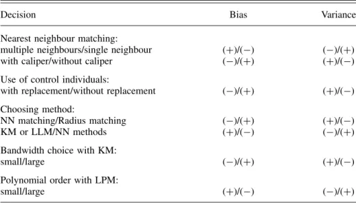
Table 1. Trade-offs in Terms of Bias and Efficiency.

Decision Bias Variance

Nearest neighbour matching:

multiple neighbours/single neighbour (+)/(−) (−)/(+)

with caliper/without caliper (−)/(+) (+)/(−)

Use of control individuals:

with replacement/without replacement (−)/(+) (+)/(−) Choosing method:

NN matching/Radius matching (−)/(+) (+)/(−)

KM or LLM/NN methods (+)/(−) (−)/(+)

Bandwidth choice with KM:

small/large (−)/(+) (+)/(−)

Polynomial order with LPM:

small/large (+)/(−) (−)/(+)

KM, kernel matching, LLM; local linear matching; LPM, local polynomial matching NN, nearest neighbour; increase; (+); decrease (−).

trade-off arising. High bandwidth values yield a smoother estimated density function, therefore leading to a better fit and a decreasing variance between the estimated and the true underlying density function. On the other hand, underlying features may be smoothed away by a large bandwidth leading to a biased estimate. The bandwidth choice is therefore a compromise between a small variance and an unbiased estimate of the true density function. It should be noted that LLM is a special case of local polynomial matching (LPM). LPM includes in addition to an intercept a term of polynomial orderp in the propensity score, e.g. p = 1 for LLM, p =2 for local quadratic matching or p = 3 for local cubic matching. Generally, the larger the polynomial orderpis the smaller will be the asymptotic bias but the larger will be the asymptotic variance. To our knowledge Hamet al.(2004) is the only application of local cubic matching so far, and hence practical experiences with LPM estimators with p≥2 are rather limited.

Trade-offs in Terms of Bias and Efficiency

Having presented the different possibilities, the question remains of how one should select a specific matching algorithm. Clearly, asymptotically all PSM estimators should yield the same results, because with growing sample size they all become closer to comparing only exact matches (Smith, 2000). However, in small samples the choice of the matching algorithm can be important (Heckmanet al., 1997a), where usually a trade-off between bias and variance arises (see Table 1). So what advice can be given to researchers facing the problem of choosing a matching estimator? It

should be clear that there is no ‘winner’ for all situations and that the choice of the estimator crucially depends on the situation at hand. The performance of different matching estimators varies case-by-case and depends largely on the data structure at hand (Zhao, 2000). To give an example, if there are only a few control observations, it makes no sense to match without replacement. On the other hand, if there are a lot of comparable untreated individuals it might be worth using more than one NN (either by oversampling or KM) to gain more precision in estimates. Pragmatically, it seems sensible to try a number of approaches. Should they give similar results, the choice may be unimportant. Should results differ, further investigation may be needed in order to reveal more about the source of the disparity (Bryson et al., 2002).

3.3 Overlap and Common Support

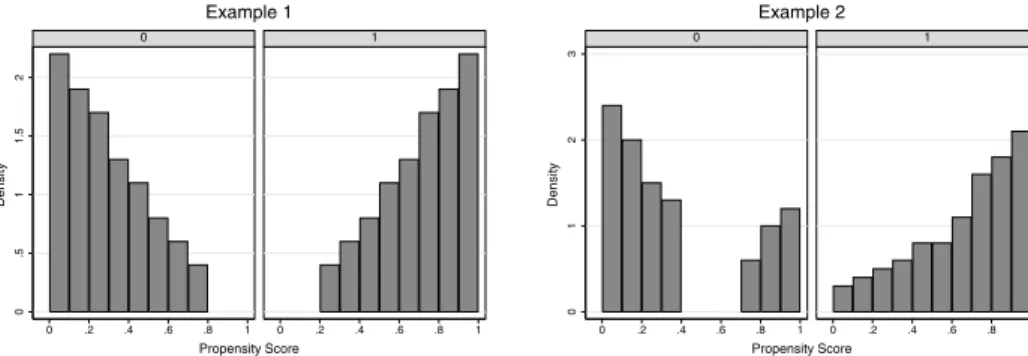
Our discussion in Section 2 has shown that ATT and ATE are only defined in the region of common support. Heckmanet al.(1997a) point out that a violation of the common support condition is a major source of evaluation bias as conventionally measured. Comparing the incomparable must be avoided, i.e. only the subset of the comparison group that is comparable to the treatment group should be used in the analysis (Dehejia and Wahba, 1999). Hence, an important step is to check the overlap and the region of common support between treatment and comparison group. Several ways are suggested in the literature, where the most straightforward one is a visual analysis of the density distribution of the propensity score in both groups. Lechner (2001b) argues that given that the support problem can be spotted by inspecting the propensity score distribution, there is no need to implement a complicated estimator.

However, some guidelines might help the researcher to determine the region of common support more precisely. We will present two methods, where the first one is essentially based on comparing the minima and maxima of the propensity score in both groups and the second one is based on estimating the density distribution in both groups. Implementing the common support condition ensures that any combination of characteristics observed in the treatment group can also be observed among the control group (Brysonet al., 2002). For ATT it is sufficient to ensure the existence of potential matches in the control group, whereas for ATE it is additionally required that the combinations of characteristics in the comparison group may also be observed in the treatment group (Brysonet al., 2002).

Minima and Maxima Comparison

The basic criterion of this approach is to delete all observations whose propensity score is smaller than the minimum and larger than the maximum in the opposite group. To give an example let us assume for a moment that the propensity score lies within the interval [0.07, 0.94] in the treatment group and within [0.04, 0.89]

in the control group. Hence, with the ‘minima and maxima criterion’, the common support is given by [0.07, 0.89]. Observations which lie outside this region are discarded from analysis. Clearly a two-sided test is only necessary if the parameter

of interest is ATE; for ATT it is sufficient to ensure that for each participant a close nonparticipant can be found. It should also be clear that the common support condition is in some ways more important for the implementation of KM than it is for the implementation of NN matching, because with KM all untreated observations are used to estimate the missing counterfactual outcome, whereas with NN matching only the closest neighbour is used. Hence, NN matching (with the additional imposition of a maximum allowed caliper) handles the common support problem pretty well. There are some problems associated with the ‘minima and maxima comparison’, e.g. if there are observations at the bounds which are discarded even though they are very close to the bounds. Another problem arises if there are areas within the common support interval where there is only limited overlap between both groups, e.g. if in the region [0.51, 0.55] only treated observations can be found.

Additionally problems arise if the density in the tails of the distribution is very thin, for example when there is a substantial distance from the smallest maximum to the second smallest element. Therefore, Lechner (2002) suggests to check the sensitivity of the results when the minima and maxima are replaced by the tenth smallest and tenth largest observation.

Trimming to Determine the Common Support

A different way to overcome these possible problems is described by Smith and Todd (2005).¹³ They use a trimming procedure to determine the common support region and define the region of common support as those values of P that have positive density within both the D =1 and D=0 distributions, i.e.

Sˆ_P= {P : ˆf(P|D=1)>0 and ˆf(P|D=0)>0} (7) where ˆf(P|D=1)>0 and ˆf(P|D=0)>0 are nonparametric density estimators.

Any P points for which the estimated density is exactly zero are excluded.

Additionally – to ensure that the densities are strictly positive – they require that the densities exceed zero by a threshold amount q. So not only the P points for which the estimated density is exactly zero, but also an additionalqpercent of the remaining P points for which the estimated density is positive but very low are excluded:¹⁴

Sˆ_Pq = {Pq: ˆf(P|D=1)>q and ˆf(P|D=0)>q} (8) Figure 3 gives a hypothetical example and clarifies the differences between the two approaches. In the first example the propensity score distribution is highly skewed to the left (right) for participants (nonparticipants). Even though this is an extreme example, researchers are confronted with similar distributions in practice, too. With the ‘minima and maxima comparison’ we would exclude any observations lying outside the region of common support given by [0.2, 0.8]. Depending on the chosen trimming level q, we would maybe also exclude control observations in the interval [0.7, 0.8] and treated observations in the interval [0.2, 0.3] with the trimming approach since the densities are relatively low there. However, no large differences between the two approaches would emerge. In the second example we