(Quantum-) critical dynamics of magnetoelectric materials
I n a u g u r a l - D i s s e r t a t i o n zur
Erlangung des Doktorgrades
der Mathematisch-Naturwissenschaftlichen Fakultät der Universität zu Köln
vorgelegt von
Christoph Grams
aus Bergisch Gladbach
Köln, 2016
Berichterstatter: Prof. Dr. Joachim Hemberger Prof. Dr. Markus Braden Vorsitzender der Prüfungskommission: Prof. Dr. Simon Trebst
Tag der mündlichen Prüfung: 25.11.2015
Contents
Introduction 1
1 Basics 3
1.1 Polarization dynamics . . . 3
1.1.1 Hysteresis loops . . . 4
1.1.2 Relaxations . . . 5
1.1.3 Ferroelectric phase transitions . . . 5
1.2 (Non-)Linear response theory . . . 6
1.2.1 Linear response theory . . . 6
1.2.2 Non-linear response theory . . . 6
1.3 Lorentz oscillator model . . . 8
1.3.1 Resonance frequency and relaxation time . . . 9
1.4 Model functions for dielectric spectra . . . 10
1.5 Temperature dependence of dielectric spectra . . . 10
1.6 Quantum paraelectrics . . . 13
1.6.1 Barrett formula . . . 13
1.6.2 Nearly constant loss . . . 13
1.7 Multiferroics and magnetoelectric materials . . . 15
1.7.1 Dzyaloshinskii-Moriya interaction . . . 15
1.7.2 Multiferroics . . . 16
1.8 Magnetic monopoles . . . 17
1.8.1 Dirac monopoles . . . 17
1.8.2 ’t Hooft monopoles . . . 17
1.9 Piston effect . . . 17
2 Experimental minutiae 19 2.1 Sample preparation . . . 19
2.2 Sawyer-Tower circuit . . . 20
2.2.1 Hysteresis loops . . . 21
2.2.2 Pyro-Current . . . 21
2.3 Measuring the complex dielectric function . . . 21
2.3.1 Impedance spectroscopy . . . 21
2.3.2 Vector network analysis . . . 22
2.3.3 Calculation ofεfromZ . . . 25
2.4 Heating effects due to electric ac currents . . . 25
2.5 Open-Short-Load calibration for the Novocontrol Alpha-A Analyzer 27 2.6 Demagnetization . . . 27
2.6.1 Notation of magnetic fields . . . 28
2.7 Cooling devices . . . 29
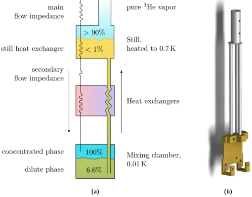
2.7.1 4He cryostat . . . 29
2.7.2 3He/4He dilution refrigerator . . . 29
Contents
3 TbMnO3 35
3.1 Introduction . . . 35
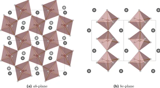
3.2 The perovskite structure . . . 36
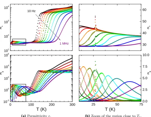
3.3 Low frequency measurements . . . 38
3.3.1 Temperature dependence . . . 38
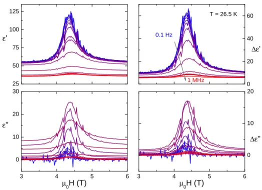
3.3.2 Magnetic field dependence at 26.5 K . . . 41
3.4 High-voltage measurements . . . 42
3.5 High-frequency measurements . . . 47
3.6 Conclusion . . . 50
4 LiCuVO4 51 4.1 Introduction . . . 51
4.2 Theoretical description and literature . . . 54
4.3 Magnetization . . . 56
4.4 Dielectric characterization . . . 58
4.4.1 H k[001], Ek[100] . . . 58
4.4.2 H k[100], Ek[001] . . . 63
4.5 Phase diagrams . . . 68
4.6 Fluctuation dynamics . . . 69
4.6.1 H k[001], Ek[100] . . . 69
4.6.2 H k[100], Ek[001] . . . 75
4.7 Conclusion . . . 79
5 Dy2Ti2O7 81 5.1 Introduction . . . 81
5.2 The pyrochlore structure . . . 84
5.3 Sample preparation . . . 85
5.4 Demagnetization correction . . . 86
5.5 Quantum paraelectic properties . . . 87
5.5.1 Nearly constant loss . . . 88
5.6 Dynamics of Magnetic Monopoles . . . 90
5.6.1 The thermodynamic limit: ν→0 Hz . . . 90
5.6.2 Peak position and relaxation time: critical speeding up . . 91
5.6.3 Broadening of the peak . . . 94
5.6.4 Relaxation strength ∆ε& the dielectric backgroundε∞ . . 94
5.7 Comparison to the magnetic ac susceptibility . . . 97
5.8 Polarization measurements . . . 99
5.9 Magneto-electric coupling in Dy2Ti2O7. . . 99
5.10 Conclusion . . . 102
6 Y2Ti2O7 103 6.1 Introduction . . . 103
6.1.1 Sample preparation . . . 103
6.2 Temperature-dependent permittivity . . . 103
6.2.1 Quantum paraelectric behavior . . . 105
6.3 Conclusion . . . 107
Summary 109
Appendix 112
iv
A Basics 113 A.1 Binomial coefficients . . . 113 A.2 Temperature-dependent dielectric spectra . . . 114
B Experimental minutiae 115
B.1 The Open-Short-Load calibration in detail . . . 115 B.2 Generalized calibration method . . . 118 B.3 Mathematica script for the demagnetization correction . . . 120
C LiCuVO4 123
Bibliography 131
Danksagung 135
Partial publications 137
Other publications 137
Abstract 139
Kurzzusammenfassung 141
List of symbols
log(x) : natural logarithm
log10(x) : common logarithm
P V R
: Cauchy principal value of an integral
ν : ordinary/technical frequency
ω= 2πν : angular/radial frequency
Z=Z0+ iZ00 : complex impedance ε=ε0−iε00 : complex dielectric function
ε∞ : contribution to ε0 from processes at higher
frequencies
C0=ε0·A/d : geometric capacitance with areaAand thick- nessd
Psw, Psat,Prem : switchable, saturation, and remanent polar- ization
Eac : amplitude of an electric ac field
Ecrcv : coercive field
M : magnetization
H =Hexternal : external magnetic field strength
Hi=Hinternal=H−DM : internal magnetic field strength with demag- netization factorD
Bi=Binternal=µ0(Hi+M) : magnetic flux density kB= 1.380 62×10−23J K−1 : Boltzmann constant ε0= 8.854×10⁻¹²A s V−1m−1: vacuum permittivity µ0= 4π×10−7V s A−1m−1 : vacuum permeability
Introduction
Magnetoelectrics are materials characterized by a coupling between their magnetic and dielectric properties, namely magnetizationM and polarizationP. This cou- pling can be of different forms and origins, some of which will be explained in the introductory chapters of this thesis.
Merely the existence of such a connection between two different physical proper- ties offers, on top of purely academic interest in the nature of the coupling, many interesting possibilities for applications. The most often named idea concerning magnetoelectric materials is data storage. Here the advantages of materials com- bining magnetic and electric properties are easily understood. For all mobile de- vices, laptop computers, mobile phones, etc., their battery life, measured in current
· time, is one of their key features. These devices also have a common capacity, the need to store data. Because a current is required in order to write or read magnetically stored data this is very energy consuming when using conventional magnetic storage media. But magnetic storage also has a very important benefit:
the lifetime of magnetic domains is much larger compared to electric domains and the stored data is retained for a very long time.
Today storage devices already use the giant magneto resistance effect where the resistance of a material depends on the relative magnetization direction of two ferromagnetic layers separated by a non-magnetic spacer. Here the data is still stored via arrangement of magnetic domains using a high current, but reading the information can be done by measuring the resistance, which only requires a very small current.
Magnetoelectric and multiferroic materials would improve this advantage even further, because they remove the need for a current to save the data. A high electric field E could be used to store data by switching the magnetization M while a lower electric field would we sufficient to read the information. Due to the coupling between polarization and magnetization the retention time in this case would be similar to purely magnetic storage.
But not only the potential to store data cheap, i.e. without investing much battery current, but also the time required to store any meaningful amount of data is important. This is where the most prominent measurement technique in the work comes in, the dielectric spectroscopy. Here electric ac voltages of differ- ent frequencies and amplitudes can be applied to the sample while measuring its response. This can be used to find the maximum frequency where the polarization of the sample can be switched with a given voltage and thereby measuring the possible write speed of the materials.
The aim of this thesis was not a specific application of magnetoelectric materials but instead the focus is on purely academic aspects of the fluctuation dynamics in the critical regime close to phase transitions. Most of the materials in this work only gain their magnetoelectric character at very low temperatures, where in this case “very low” means temperatures well below 10 K. The truly novel and unexpected phenomena can only be observed at temperatures even lower than this by more than one order of magnitude.
The required low temperature itself was one of the most challenging aspects
Contents
during the experimental work presented in this thesis. Additionally, measurements of the dielectric properties at frequencies of the order of 100 MHz and higher are subject to many error sources, for example the change of the cable length and resistivity while cooling. Their sensitivity towards this undesired effects only increases when working towards higher frequencies.
This work was supported by the DFG through SFB 608, research grant HE- 3219/2-1, and the “Quantum Matter and Materials” (QM2) Center of Excellence at the University of Cologne.
2
1 Basics
On the next pages the basic concepts that are the foundation of this work are briefly introduced. Mostly a short review is given, only for few topics some math- ematical deliberations are presented that will be important for the evaluation of the experimental data.
Contents
1.1 Polarization dynamics . . . . 3
1.1.1 Hysteresis loops . . . 4
1.1.2 Relaxations . . . 5
1.1.3 Ferroelectric phase transitions . . . 5
1.2 (Non-)Linear response theory . . . . 6
1.2.1 Linear response theory . . . 6
1.2.2 Non-linear response theory . . . 6
1.3 Lorentz oscillator model . . . . 8
1.3.1 Resonance frequency and relaxation time . . . 9
1.4 Model functions for dielectric spectra . . . . 10
1.5 Temperature dependence of dielectric spectra . . . . 10
1.6 Quantum paraelectrics . . . . 13
1.6.1 Barrett formula . . . 13
1.6.2 Nearly constant loss . . . 13
1.7 Multiferroics and magnetoelectric materials . . . . . 15
1.7.1 Dzyaloshinskii-Moriya interaction . . . 15
1.7.2 Multiferroics . . . 16
1.8 Magnetic monopoles . . . . 17
1.8.1 Dirac monopoles . . . 17
1.8.2 ’t Hooft monopoles . . . 17
1.9 Piston effect . . . . 17
1.1 Polarization dynamics
In general three different mechanisms of electrical polarization are observed in crystals. The origins of these processes are, in the order of their typical resonance frequencies:
• electronic - caused by the shifting of the electrons with respect to the atomic core
• ionic - movement of oppositely charged ions in different directions with op- tical phonons
• orientation - shift of the orientation of existing dipoles
1 Basics
ε’,ε’’
ν ( a . u . )
F 7 6
P r o b e K o m m e n t a r
orientational ionic electronic
Figure 1.1:
Polarization processes in spectroscopic measure- ments.
Schematic representation of different polarization pro- cesses typically observed with spectroscopic measurements.
P
E
(a)
P
E r
Ecrcv rPsat
rPrem
(b)
Figure 1.2:Sketch of a hysteresis loop.
(a) A typical hysteresis loop as could be measured in a ferroelectric material.
(b) The same hysteresis loop without the slope caused byε0 . In the inset the distinction betweenPsat and Prem can be seen more clearly.
Figure 1.1 shows a schematic representation of the previously mentioned mech- anisms of polarization dynamics. The relaxational processes associated with shifts of dipol orientation are typically the slowest mechanism observed and are char- acterized by high damping. Faster are ionic and electronic contributions but for the frequency range discussed in this thesis, 10 GHz and below, they cause only a frequency-independent offset in the permittivityε0 that is calledε∞.
1.1.1 Hysteresis loops
Typically, electrical polarization is observed by either measuring the pyroelectric current P(T) or, at constant temperature, the electric-field dependence of the polarization P(E). In the scope of this section the general form of the latter curves is discussed as some knowledge of the terminology regarding hysteresis loops is required for the discussion of the experimental results in chapters 4 and following.
A generic hysteresis loop as could have been measured in a ferroelectric material is shown in figure 1.2a. Before analyzing the actual hysteresis loop the slope observed in the saturation regime has to be taken into account. This slope is
4
caused by the dielectric constantε0 of the material and the latter can be calculated from the slopesin the linear regime on both sides of the curve using
s= dP
dE =χ·ε0= (ε0−1)·ε0. (1.1) After subtracting this slope the hysteresis loop has the more common form shown in figure 1.2b where some points are of special interest. First the saturation polarizationPsat,i.e. the maximum value ofP realized for strong electric fields.
This can be found from theP-intercept of fits in the linear regime. Slightly lower than Psat is the remanent polarization Prem that denotes the polarization value measured at E = 0 after reaching the saturation polarization. On the electric- field axis the coercive fieldEcrcvis the field value that is required to suppress the remanent polarization,i.e. P(Ecrcv) = 0. This can be understood as a measure of the stability of the ferroelectric phase against perturbations bye.g. temperature induced disorder.
1.1.2 Relaxations
Opposed to both electronic and ionic polarization the orientation polarization requires the existence of permanent dipole moments that try to reorient in the applied electric ac field due to a (small) time-dependent inhomogeneity induced into their potential. This leads to a time dependence of the polarization that is driven by the difference between the polarizationP(t) at timetand the equilibrium polarizationP∞(t) that would be observed if the system were to stay at the current voltage for infinite time:
dP(T)
dt =−P(t)−P∞(t)
τ (1.2)
The relaxation timeτ of the thermally activated reorientation can be given as
τ=τ0ekUBbT (1.3)
where τ0 is the time between two tries to change the orientation by passing the potential barrierUb.
1.1.3 Ferroelectric phase transitions
Ferroelectricity can be induced by two different mechanisms. The order-disorder transition where the polarization is present in both the ferroelectric and the para- electic phase and only its long-range order is lost when crossingTc, resulting in a vanishing net polarization. Secondly, the displacive phase transition where the shifting of two sublattices with differently charged ions in opposite directions cre- ates net polarization during this structural phase transition.
Critical slowing down / soft phonon modes
Ionic polarization can only be observed with low frequencies close to a displacive (anti-)ferroelectric phase transition when the transverse optical phonon branch slows down into the measurable frequency range.
This behavior is called critical slowing down and the corresponding phonon mode is called soft [5]. In terms of a description with critical exponents,
1 Basics
1/τ ∝2πνp∝ |T−Tc|γ this behavior is described with a positive exponentγ >0.
Magnetic field as control parameter
If a magneto-electric coupling exists a ferroelectric phase transition can also be driven by the magnetic field because in this case the energy barrierUbin equation (1.3) depends on the magnetic field. Changing the magnetic field at constant temperature now has essentially the same influence onτ as the temperature at constant - or zero - magnetic field. An example for this behavior is the multiferroic MnWO4 where the critical dynamics has recently been studied [64, 63]. Here it was shown that the critical dynamics at the phase transition are independent of the control parameter used to drive the transition.
1.2 (Non-)Linear response theory
The interaction of electromagnetic waves with matter can be described theoreti- cally as perturbations and lead to the response functionsε(k, ω) andχ(k, ω) that depend on the momentum and the frequency of the electromagnetic wave.
As the highest frequencies used for the spectroscopic measurements presented in this work are in the GHz range the corresponding wavelength1 is clearly much larger than the atomic length scale of any sample. Thus, the momentum depen- dence can be ignored andkis assumed to be zero for the following deliberations.
Furthermore, using specific geometries of the sample holder it can be selected whether the electric or magnetic component couples to the sample. Therefore, it is sufficient to consider this argument only for eitherε(ω) orχ(ω), here the latter will not be discussed in detail.
Depending on the strength of the perturbation, in this case the amplitude of the electric ac field, this description can be done in two limits that will be described in the following two sections.
1.2.1 Linear response theory
If the applied electrical field E is small enough the polarization P(E) can be described as a linear function ofE: P(E) ∝E and terms of higher order in E can be ignored. In this case the dielectric constant is independent of the actual strengthE of the electric field: ε= dP/dE∗1/ε0+ 1.
1.2.2 Non-linear response theory
Once the applied electrical field is high enough a linear description of P(E) is insufficient and the higher order terms have to be taken into account:
P(E) =α1ε0E+α2ε0E2+α3ε0E2+...=ε0
∞
X
n=1
anEn.
When applying an oscillating electrical fieldE(t) =Eacsin(ωt) the expression for the polarization can be written as
110 GHz translate to a wavelength of 29.98 mm≈3 cm in vacuum.
6
P(t) =ε0Eac
∞
X
n=1
anEac(n−1)sinn(ωt) =ε0Eac
∞
X
n=1
anEac(n−1)in
2n e−iωt+ eiωtn
. Using the binomial expansion this equation can be rewritten as
P(t) =ε0Eac
∞
X
n=1
aninEac(n−1)
2n
n
X
k=0
n k
e−i(n−k)ωt+ikωt
=ε0Eac
∞
X
n=1
ani(n−1)E(n−1)ac
2n
n
X
k=0
n k
ie−i(n−2k)ωt. (1.4)
Due to the symmetry of the binomial coefficients and the exponential function2 the latter sum can be reduced to half its elements:
P(t) = Re
ε0Eac
∞
X
n=1
ani(n−1)E(n−1)ac
2n
<n/2
X
k=0
2n k
ie−i(n−2k)ωt
+Peven
where the time-independent contributions fork=n/2 from evennare combined intoPeven and only the real part is taken into account.
From this equation two things can be derived. First, contributions from even and oddndo not mix, as only multiples of 2 are subtracted from n. Secondly the contributions for even n produce a contribution that is independent of ωt when k=n/2.
Sorting the elements of the summation by the multiple (n−2k) ofω and com- bining the corresponding prefactors into a common factor calledεn while keeping in mind that only the real part of the polarization is relevant leads to
P(t) = Re
"
ε0Eac
∞
X
n=1
εnie−inωt
#
=ε0Eac
∞
X
n=1
ε0nsin(nωt)−ε00ncos(nωt). (1.5) Thus the hysteresis curve of the sample can be evaluated by measuring the polarization for integer multiples of the excitation frequency.
As hysteresis curves in general are centered around the point of origin and no offset is observed this indicates that the even contributions of this expansion are expected to be small or vanish. This is also consistent with the point symmetry of theP(E) curves,P(E) =−P(−E), that is consistent only with the symmetry observed for odd exponents inE.
For the model case of a perfectly rectangular hysteresis loop it was argued in [63]
that the first order harmonic contributions,ε01 andε001, can be used to calculate both the switchable polarizationPsw and the coercive fieldEcrcv:
2This argument can be found in the appendix A.1 on page 113 in more detail.
1 Basics
|∆ε1|=q
(ε01−ε∞)2+ε0021 Psw= π
4ε0|∆ε1|Eac (1.6)
Ecrcv= ε001
|∆ε1Eac (1.7)
Using this relations with measured data will provide a good approximation of bothPsw and Ecrcvas long asEac> Ecrcv.
1.3 Lorentz oscillator model
A simple model for the description of the polarization mechanisms introduced in section 1.1 is the Lorentz3 oscillator model. This standard model of electrical polarization can be found in many textbooks,e.g. [28]. It describes the frequency- dependent permittivity as a sum over many resonant processes:
ε= 1 +X
s
nse2
ε0ms· 1 ω20,s−ω2+ iωΓs
(1.8) with
ns in m−3 : number of electrons per volume ω0,s in s−1 : resonant frequency
e in C : charge of the electron ms in kg : effective mass
ω in s−1 : operating angular frequency of the measurement Γs in s−1 : damping factor
For the low frequency limit the contributions of all faster processes can be as- sumed to be constants and are combined intoε∞ in the following. This reduces equation (1.8) to
ε= ne2
ε0m · 1
ω02−ω2+ iωΓ+ε∞ (1.9) leaving only the polarization mechanism in the measured frequency range. Divid- ing this equation into its real and imaginary part leads to equations (1.10a) and (1.10b) using the definition ofε=ε0−iε00.
ε0 = ne2
ε0m· ω02−ω2
(ω02−ω2)2+ω2Γ2 +ε∞ (1.10a) ε00= ne2
ε0m · ωΓ
(ω02−ω2)2+ω2Γ2 (1.10b) The quotient of real and imaginary part, called the loss angle tan(δ), is also useful to see a change in damping or resonance frequency:
tan(δ) = ε00
ε0−ε∞ = Γω
ω20−ω2. (1.11)
3The model is named after Hendrik Antoon Lorentz, * 18.07.1853, † 04.02.1928, who received the Nobel Prize in Physics in 1902 together with Pieter Zeeman for their discovery and explanation of the Zeeman effect.
8
0 . 1 1 1 0 1 0 0 1 E - 4
1 E - 3 0 . 0 1 0 . 1
1
ω2r/ω20
h i g h d
a m p i ng l o w d a m p i n g
ω2 r /ω2 0
γ = Γ/ω0
Figure 1.3:
Resonance frequency of a damped Lorentz oscilla- tor.
The dependence of the reso- nance frequencyω2r/ω20on the dampingγ= Γ/ω0as given in equation (1.13). In the case of low damping, γ 1, the resonance frequency is identi- cal toω0. For high damping theγ dependence is found as ω2r/ω20∝1/γ2.
1.3.1 Resonance frequency and relaxation time
With this model the dependence of the resonance frequencyωron both the damp- ing Γ and the undamped eigenfrequencyω0can be calculated from the zero of the first derivative of the dielectric loss in equation (1.10b):
dε00
dω = Γω40+ 2ω02ω2−3ω4−Γ2ω2 ((ω02−ω2)2+ Γ2ω2)2 = 0.
Solving this equation forω02 leads to two solutions, one of which is always neg- ative and will be ignored as non physical. The remaining solution
ω02=p
4ωr4+ Γ2ωr2−ω2r (1.12) is always positive and yields the expected result ω02 = ω2r for the limit of non damping (Γ = 0).
To study the influence of the damping on the resonance frequency in more detail equation (1.12) is solved forωr2:
ωr2=−Γ2+p
Γ4−4Γ2ω02+ 16ω40+ 2ω02
6 .
By introducing a normalized damping factorγ= Γ/ω0the resonance frequency ωr can be expressed in units ofω0,
ωr2
ω02 = −γ2+p
γ4−4γ2+ 16 + 2
6 . (1.13)
This result is plotted in figure 1.3 in combination with plots showing the limits of low and high damping.
For very high damping,γ1 (Γω0), as expected in all relaxation processes, equation (1.13) yields
ω2r
ω20 =γ−2= Γ
ω0
−2
as can also be seen in figure 1.3. Further simplification yields 2πνr=ωr=ω20
Γ = 1
τ (1.14)
with the characteristic relaxation timeτ of the system.
1 Basics
1.4 Model functions for dielectric spectra
Assuming a high damping factor, Γω0, equation (1.9) can be simplified using (1.14). After bracketingω02in the denominator, defining ∆ε=ne2/(ε0mω20) , and settingω2/ω20≈0 due to the high damping this leads to the most common model function for dielectric spectra, the Debye function
ε(ω) = ∆ε
1 + iωτD +ε∞ (1.15)
with
∆ε: dielectric relaxation strength τD : Debye relaxation time
where τD can be calculated from the peak position νP in the dielectric loss by 2πνP= 1/τD.
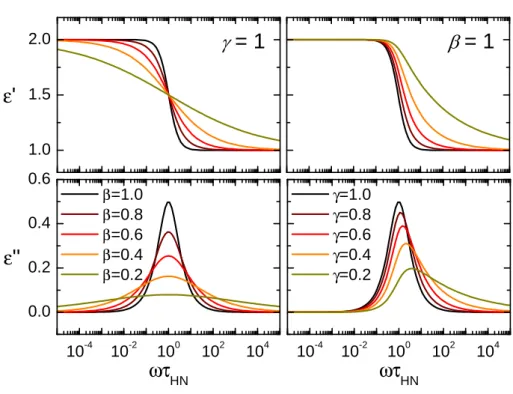
If a distribution of several contiguous relaxation times is observed they can either be described by a sum of Debye relaxations or with a single empirical model function. The most general model function is the Havriliak-Negami function [31]:
εHN(ω) = ∆ε
1 + (iωτHN)βγ +ε∞ (1.16) β : symmetric peak broadening, 0< β ≤1
γ : asymmetric peak broadening, 0< βγ≤1
the exponentsβ andγlead to a broadening of the peak in the dielectric loss, the influence of the exponents on the form of the curves can be seen in figure 1.4.
Opposed toτDthe relaxation timeτHNis not directly related to the peak position in the dielectric loss but depends on the parametersγ andβ [47]:
2πνP= 1 τHN
sin βπ 2 + 2γ
1/γ
sin βγπ 2 + 2γ
−1/β
. (1.17)
Other model functions can be deduced from the Havriliak-Negami function by setting one of the exponentsγorβ to one. Withγ= 1 equation (1.16) is changed into the Cole/Cole function. β = 1 reduces the Havriliak-Negami function to the Cole/Davidson function. If both exponents are one the Havriliak-Negami function and the Debye function are identical.
1.5 Temperature dependence of dielectric spectra
Not only the frequency dependence of the dielectric function is of interest but also its temperature dependence. For further analysis an assumption has to be made where to enter the temperature dependence into the Debye function, equation (1.15). Here we assumeτ(T) to be depending on the temperature T via a typical temperature activated process,
τ=τ0ekUBbT, (1.18)
with τ0 and the potential barrier Ub as previously mentioned in section 1.1.2.
Using this approach the Debye function now has the more complicated form
10
1 . 0 1 . 5 2 . 0
ε ’
1 0 - 4 1 0 - 2 1 0 0 1 0 2 1 0 4
0 . 0 0 . 2 0 . 4 0 . 6
β= 1 . 0 β= 0 . 8 β= 0 . 6 β= 0 . 4 β= 0 . 2
ε ’ ’
ωτ
H N = 1
1 0 - 4 1 0 - 2 1 0 0 1 0 2 1 0 4
γ= 1 . 0 γ= 0 . 8 γ= 0 . 6 γ= 0 . 4 γ= 0 . 2
ωτ
H N = 1
Figure 1.4:Influence of β and γ on the Havriliak-Negami function.
Plot of the Havriliak-Negami function withγ= 1 (Cole/Cole function) on the left and β = 1 (Cole/Davidson function) on the right. The black line ( ) in all plots (γ=β= 1) represents the Debye function.
1 Basics
ε’
ωτ0 = 0 . 0 3 2
0 . 3 2 0 . 1
0 . 0 0 . 5 1 . 0 1 . 5 2 . 0
ε’ ’
T / ( U
b/ k
B )
D e b y e v s T
ε∞ + ∆ε
ε∞
∆ε / 2
0
Figure 1.5:
Temperature-dependent Debye relaxation.
Both real (upper panel) and imaginary part (lower panel) of the complex dielectric function ε(ω, T) given in equation (1.19) for different normalized frequencies τ0ω as function of normalized temperature T in units of Ub/kB. The real part shows a step with a corresponding peak in the imaginary part.
For higher frequencies both step and peak are shifted to higher temperatures and less well-defined.
ε(ω, T) = ∆ε
1 + iωτ0ekUBbT +ε∞. (1.19) For further analysis this complex function is separated into its real and imaginary part
ε0(ω, T) = ∆ε
1 +ω2τ02ek2UBbT +ε∞, ε00(ω, T) =− ∆εωτ0ekUBbT 1 +ω2τ02ek2UBbT
where the latter is expected to have a maximum. To find the position of this maximum the zero of the first derivative of the imaginary part with respect toT can be calculated as
Tmax=−Ub
kB
· 1
log (τ0ω). (1.20)
More details on this can be found in appendix A.2 on page 114.
Figure 1.5 shows a plot of both real and imaginary part of equation (1.19) for different normalized frequenciesτ0ωas a function of the temperature in units of the activation energyUb/kB. The logarithmic spacing in the normalized frequencies was chosen to show as broad a range of different curves as possible and was inspired by equation (1.20) that predicts a logarithmic spacing of the maxima with respect to τ0ω. In real systems not only the relaxation time but also the ∆ε may vary withT and its temperature dependence is harder to model.
12
1.6 Quantum paraelectrics
Quantum paraelectric materials are characterized by a non vanishing dielectric function atT →0 K that is caused by quantum fluctuations. The name quantum paraelectic has been introduced by Müller and Burkhard [58] who researched the dielectric function of SrTiO3at temperatures down to and below 4 K. They found that the quantum fluctuations causing the high value ofε0 are ferroelectric fluc- tuations. As the transition temperature in to the ferroelectric phase is expected forT <0 K quantum paraelectic materials are also called incipient ferroelectrics.
1.6.1 Barrett formula
In 1952 Barret [3] proposed a formula to describe the temperature dependence of quantum fluctuations that was derived forχ0 in [34]:
χ0= nkBµ2 Ω
2kB
coth
Ω 2kB· T1
−4kJ0
B
(1.21) with
Ω/kB : integral of the tunneling probability n : dipole density
µ : dipole strength J0/kB : J0=P
jJij effective coupling constant
In the limit of Ω→0 all quantum fluctuations vanish and the equation is reduced to
Ω→0limχ0= nk2Bµ2
kBT−J0/4, (1.22)
because lim
x→0x·coth (x/a) =a.
IdentifyingT0 withJ0/4kB this equation matches the Curie-Weiss law:
Ω→0limχ0= nkBµ2
T−T0 = C
T−T0. (1.23)
1.6.2 Nearly constant loss
A second property discussed in connection with quantum paraelectic materials is the so-called nearly constant loss behavior, meaning that the dielectric loss is observed to have a nearly constant value grater zero over a wide frequency range. In the following section this assumption will be examined theoretically after introducing the Kramers-Kronig relations that are a necessary tool for this considerations.
Kramers-Kronig relations
A functionf(z) is complex analytic on an open setD in the complex plane if for anyz0in D one can write
f(z) =
∞
X
n=0
an(z−z0)n
1 Basics
in which the coefficientsan are complex numbers and the series is convergent to f(z) for z in a neighborhood ofz0 [73]. For every function that is complex ana- lytic in the upper half-plane the Kramers-Kronig relations describe the correlation between real and imaginary part of said function. Due to the implication of analyt- icity by causality the Kramers-Kronig relations are valid for all response functions of physical systems [89].
The most common notation of the Kramers-Kronig relations, founde.g. in [47], is
ε0(ω)−ε∞= 2 πP V
ω0
Z
0
uε00(u)
u2−ω2 ·du (1.24)
where the Cauchy principal value (P V) of the integral has to be used to integrate over the divergence atω=u.
A more convenient representation of the Krames-Kronig relations for ε that does not rely on the Cauchy principal value is given in equations (1.25), that were derived for the complex ImpedanceZ in [6].
ε0(ω)−ε∞= 2 π
ω0
Z
0
uε00(u)−ωε00(ω)
u2−ω2 ·du (1.25a)
∆ε= 2 π
ω0
Z
0
ε00(u)
u ·du (1.25b)
ε00(ω) =−2ω π
ω0
Z
0
ε0(u)−ε0(ω)
u2−ω2 ·du (1.25c)
δ(ω) =2ω π
ω0
Z
0
log|ε(ω)|
u2−ω2 ·du (1.25d)
Many spectroscopic measurement methods rely on the Kramers-Kronig rela- tions to get information on the complex response function while measuring e.g.
only absolute values without phase information. While this is not the case for the measurements presented in this work it can be quite instructional to use the Kramers-Kronig relations to examine the influence of simple assumptions for the dielectric lossε00 onε0 as shown in the following section.
Kramers-Kronig and constant loss
If the dielectric lossε00=a·ω+bis assumed to be a linear function for frequencies below ωL and still satisfies the analyticity condition for all frequencies up to ω0
equation (1.25a) becomes
ε0(ω)−ε∞=2 π
ωL
Z
0
u(a·u+b)−ω(a·ω+b) u2−ω2 ·du +2
π
ω0
Z
ωL
uε00(u)−ωε00(ω)
u2−ω2 ·du (1.26)
14
1 0- 4 1 0 - 3 1 0 - 2 1 0 - 1 1 00
0123
a p p r o x i m a t i o n f u l l r e s u l t
ε’/ε’’
ω/ωL C o n s t a n t l o s s
Figure 1.6:
Permittivity for a con- stant loss material.
Plot of the Kramers-Kronig equation (1.29) for a constant loss scenario with the slope a and all constant terms set to zero. The constant loss leads to a change ofε0(ω) that is proportional to −log(ω) if ωωL.
The second integral yields a finite value that will be calledc(ω) in the following while the first integral can be solved:
ε0(ω)−ε∞= 2 π
ωL
Z
0
u2a+ub−ω2a−ωb
u2−ω2 ·du+c(ω)
= 2 π
a(u+ω) +blog (u+ω)ωL
u=0
+c(ω)
= 2 π
a(ωL+ω) +blog
ωL+ω ω
+c(ω)
=−2b πlog
ω ωL+ω
+2a(ωL+ω)
π +c(ω) (1.27) IfωωL than equation (1.27) can be reduced to
ε0(ω) =−2b
πlog (ω) +2 π
hblog (ωL) +a(ωL+ω)i
+c(ω) +ε∞ (1.28) where the slope a in ε00 adds both a constant offset and a linear term in ω to ε0 . c(ω) = c can be assumed to be independent of ω as long as the latter is much smaller thanωL. In the case of a constant loss witha= 0 and, therefore, b=ε00(ω) =εc.l.this equations can be further simplified to
ε0(ω) =−2εc.l.
π log (ω) + const. (1.29) The resulting function ε0(ω) is shown in figure 1.6 in comparison to the more extensive equation (1.27) (orange). Here the quality of the approximation can be assessed and only small deviations are visible as long asω.0.1ωL.
1.7 Multiferroics and magnetoelectric materials
1.7.1 Dzyaloshinskii-Moriya interaction
The Dzyaloshinskii-Moriya interaction, sometimes also called anisotropic superex- change interaction, was first postulated by Igor Dzyaloshinskii in 1958 [20].
1 Basics
From symmetry considerations based on the Landau theory he postulated the existence of a contribution to the total magnetic exchange interaction that can be written asH=Di,i+1·(Si×Si+1). Two years later Tôru Moriya [55] explained the origin of the anisotropic superexchange interaction with the spin-orbit coupling, giving the phenomenological model from Dzyaloshinskii a firm theoretical basis.
H H
HHH @I@ Si
x ri,i+1
Si+1 6
s ? c
r b
s c Figure 1.7: Effects of the Dzyaloshinskii-Moriya interac- tion.
The effects of the Dzyaloshinskii-Moriya in- teraction are sketched in figure 1.7. The Dzyaloshinskii vectorDi,i+1 is proportional to the spin-orbit coupling constant and the posi- tionxof the superexchange ion, typically O2−, the open circle in the sketch. Therefore, the anisotropic superexchange can shift the posi- tion x of the superexchange ion and slightly deform the crystal structure and in some cases
breaking the inversion symmetry and creating an electric dipole moment. The latter only happens in spiral spin states where the induced dipole momentPcan be expressed as
P∝ri,i+1×(Si×Si+1).
In non-spiral spin configurations the spin current ji,i+1 = Si×Si+1 does not have the same sign for allithus the sum of allji,i+1 vanishes.
More comprehensive information on the Dzyaloshinskii-Moriya interaction can be founde.g. in [13].
1.7.2 Multiferroics
In general multiferroics are materials that combine any two or more ferroic prop- erties,i.e. ferroelectric, ferromagnetic, ferrotoroidicity, or ferroelasticity. Though typically only the coexistence of ferromagnetic and ferroelectric ordering is thought of when calling a material multiferroic.
In this case not only a coupling, e.g. P ∝ H, exists but both P and M are switchable equally byH orE.
Type I
Type I multiferroics are materials where the ferromagnetic and ferroelectric are caused by separate effects and in general also exhibit different transition temper- atures. For this materials the coupling between ferromagnetic and ferroelectric is very weak.
Type II
For the type II multiferroics this is not true. Here the magnetic order causes the ferroelectric behavior and a strong coupling exists between the magnetic and electric properties. The downside of type II multiferroics is their weak polarization, that is smaller compared to canonical ferroelectric materials by four orders of magnitude.
For more information on multiferroic materials seee.g. [13, 38]
16
1.8 Magnetic monopoles
The search for magnetic monopoles has its origin in the symmetry of the field equations of electrodynamics with respect to electric and magnetic field. However, the symmetry between both fields is disturbed by the absence of experimental prove of a single magnetic charge on a particle.
1.8.1 Dirac monopoles
This problem was studied by Dirac in the 1930s and in the course of 20 years he published several papers [17, 18] on this topic. In [18] he summarizes his ideas that will be roughly explained in the following.
The typical approach to the vector potential in magnetism,
F=∇ ×A (1.30)
only works if there are no magnetic monopoles. In this case equation (1.30) also means that for any closed surface at any moment the flux through this surface has to vanish.
If there exists a magnetic monopole this cannot be true for any surface of a volume that contains the monopole, e.g. a sphere centered on the monopole, as the magnetic flux from the monopole cannot vanish. But it can be assumed that the flux from the monopole only crosses the surface at one point for each closed surface surrounding the monopole. Tracing this point through space as the volume expands leads to the so called Dirac string that connects the monopole either with infinity or with their corresponding anti monopole. The key to Dirac’s theory is that the strings are invisible for the magnetic monopoles and their length does not influence the monopoles. For this reason the strings are sometimes also called tensionless.
1.8.2 ’t Hooft monopoles
A different approach on magnetic monopoles was introduced by ’t Hooft in [35]
were he showed that the Dirac string is not necessary in gauge theories where the electromagnetic group is a subgroup of a larger group with compact covering group.
While ’t Hooft monopoles are closer to the intuitive notion of a monopole than the Dirac monopoles as they can be seen as single entities they are only mentioned here for the sake of completeness. For the experimental work in this thesis only the former type of monopoles is important.
1.9 Piston effect
In the early 1990s the critical properties of liquids close to the critical point of their liquid-gas transition have been studied [7, 66, 94]. The focus of these studies was the thermal equilibration of3He in zero gravity that were experimental observed [14] to be much faster than expected. This was explained by the adiabatic change of temperature and density in compressible liquids. Close to the critical point this process dominates due to the divergence ofcP and the adiabatic process dominates the distribution of temperature throughout the bulk. The authors conclude that for a fixed volume of the sample cell their numerical calculations reproduce the observed critical speeding up.
2 Experimental minutiae
Following the theoretical topics in the previous chapter here the measurement techniques used will be introduced. Again, an in-depth explanation is left to liter- ature. Instead only a brief summary of the working principles of the instruments used is provided.
Contents
2.1 Sample preparation . . . . 19 2.2 Sawyer-Tower circuit . . . . 20 2.2.1 Hysteresis loops . . . 21 2.2.2 Pyro-Current . . . 21 2.3 Measuring the complex dielectric function . . . . 21 2.3.1 Impedance spectroscopy . . . 21 2.3.2 Vector network analysis . . . 22 2.3.3 Calculation ofεfromZ . . . 25 2.4 Heating effects due to electric ac currents . . . . 25 2.5 Open-Short-Load calibration for the Novocontrol Alpha-
A Analyzer . . . . 27 2.6 Demagnetization . . . . 27 2.6.1 Notation of magnetic fields . . . 28 2.7 Cooling devices . . . . 29 2.7.1 4He cryostat . . . 29 2.7.2 3He/4He dilution refrigerator . . . 29
2.1 Sample preparation
For all measurements of the polarization and related quantities such as the complex impedance the sample has to be prepared correctly before measuring. The most important consideration is the sample geometry. Besides the basic need to align the magnetic and electric fields with certain crystallographic axes the geometric capacitanceC0=ε0·A/dshould be optimized. This can be done by either reducing the thicknessdof the sample or increasing the areaAof the capacitor plates that have to be applied to both sides of the sample. The material of the capacitor plates can be varied to check for effects of contact resistance on the measurements.
For this reason a thin slab is the best option, even though depending on the orientation of the sample with respect to the magnetic field the demagnetization (section 2.6) has to be taken into account when applying a magnetic field.
Finally, the sample has to be glued on the sample holder and both sides are con- nected to the cables using silver paint. Figure 2.1 shows a sketch of the microstrip sample holder with a sample.
2 Experimental minutiae
Figure 2.1:
Sketch of the sample holder.
The external magnetic field is oriented inzdi- rection while the electric field for the depicted sample orientation is perpendicular toHalong the copper stripe.
rUt r
C sample
r r r
r r r r r
Us
Uc
Figure 2.2:
Sawyer-Tower circuit.
Simplified diagram of the Sawyer-Tower cir- cuit. The dielectric constant of the sample can be calculated from the ratio of US and UC if the value ofC is known.
2.2 Sawyer-Tower circuit
For measurements of the polarization of ferroelectric materials Sawyer and Tower [77] introduced an electric circuit that is sketched in figure 2.2.
The sample is mounted as dielectric in a plate capacitor with a reference capaci- torCof known capacity in series. Applying a voltageUtleads to a shift of charges Q=C·Uc at the reference capacitor. Due to the serial setup the same amount of charge is moved at the sample. From the evaluation of the two partial voltages UsandUc both the polarizationP and the applied electric field can be calculated from the electric displacement fieldD=Q/Aand the electric fieldE=Us/dof a plate capacitor:
E= 1 dUs
P=D−ε0E=Q
A−ε0Us d = ε0
d C
C0
Uc−Us
(2.1)
From the combination of equations (2.1) andP =χε0E+Psthe sample specific quantities can be found.
Using a reference capacitor with a much higher capacity than the sample,C Cs, and measuring both the total voltageUt=Us+Uc and the voltageUc at the reference capacity reduces the complexity of the analysis and also has additional advantages, see [32]. In this case the voltage at the sample can be approximated with the total voltageUs≈Ut.
In the original presentation of the circuit an oscilloscope was used to monitor the results. All measurements shown in this work were obtained using aKeithly
20
6517B Electrometer to measure either the charge Q for hysteresis loops or the currentI for Pyro-Current measurements.
More information on the experimental details of the Sawyer-Tower circuit used can be found in [32].
2.2.1 Hysteresis loops
From the measurement of the applied voltage Ut and the charge Q the P(E) hysteresis loop can be calculated from measurements with different voltages if the geometry of the sample is known.
IfCCsis satisfied the electric field applied to the sample can be approximated to E ≈Ut/d. Due to the serial setup of both capacitors the amount of charges moved through the circuit also has to reside on the sample and thusP =Q/A.
2.2.2 Pyro-Current
Typical pyro-current measurements are done by cooling the sample with an ap- plied electric field from the paralectric to the ferroelectric phase. This causes all ferroelectric domains in the sample to fully nucleate in an advantageous orientation with respect to the electric field and thereby maximizes the electric polarization.
Once the cooling of the sample is complete the electric field is disabled,Ut= 0.
The actual measurement of the Pyro-Current is performed during the reheating of the sample with a constant temperature drift without electric field. Both the discharge current of the fully polarized sample and the temperature are recorded as a function of time. Due to the large amounts of charge that are shifted at the ferroelectric phase transition and the technical limitations of the instrument it is more convenient to measure charge indirectly via the displacement current I= dQ/dt.
Integrating the currentI over the timetleads to the chargeQand thus also to the polarizationP =Q/A.
2.3 Measuring the complex dielectric function
To achieve as broad a frequency range as possible different measurement techniques have to be used. In the following sections the spectroscopy techniques used in this work and the methods to calculateε(ν) from the measured quantities are briefly introduced.
2.3.1 Impedance spectroscopy
For frequencies up to roughly 10 MHz impedance spectroscopy can be used to measure the complex impedance Z of the sample. In this thesis a Novocontrol Alpha-A Analyzer was used that covers a broad frequency range from 1 mHz to 10 MHz. For the measurement of the complex impedance it uses the gain-phase method that measures currentI, voltageU, and phase angleφto calculateZusing
Z= U I
In earlier measurements using the Novocontrol Alpha-A Analyzer the results were saved in an alternative form fromZ,RpandCp. Using the equivalent circuit
2 Experimental minutiae
Rp Cp
Figure 2.3:Equivalent circuit diagram: Rp and Cp.
For the calculation of Z from Rp and Cp an ideal resistor is assumed to be connected in parallel with an ideal capacitor.
diagram in figure 2.3Z can be calculated by 1/Z= 1/Rp+ i2πνCp. Solving this equation forZ0 andZ00 leads to
Z0=
1 Rp
1 Rp
2
+ (2πνCp)2
, Z00= −2πνCp
1 Rp
2
+ (2πνCp)2
. (2.2)
2.3.2 Vector network analysis
When increasing the frequency ν at some point the corresponding wavelengthλ will be equal or shorter than the length of the cables in the setup1. In this case the simple method described earlier will no longer yield accurate information on the phaseφand a different approach has to be used. This is done by using a complex network analyzer that measures the scattering parameters, which are the ratios between the amplitudes of the outgoing and incoming signal. The convention for the notation of the four scattering parameters is Ssr where the electromagnetic wave is applied at the source port s and the measurement of the reflected (r = s) or transmitted (r 6= s) wave is done at the receiver on port r. In figure 2.4 the scattering parameters are shown in a sketch. For the measurements in the higher frequency range two diveces were used. The Rhode & Schwartz ZVB4 for frequencies from 100 kHz to 4.2 GHz and the Agilent PNA-X in the range of 10 MHz to 20 GHz.
Calibration
Opposed to the measurement of the complex impedance for this measurements extensive calibrations have to be done beforehand. For the calibration the four standards open, load, short, and through are used. The first three standards are used to individually calibrate each of the semi rigid coaxial cables of the setup by changing the resistivity between the inner conductor and the outer shield at the sample location fromRopen→ ∞ via Rload = 50 W to Rshort = 0 W. Finally, the through connects the inner conductors of both cables with Rthrough = 0 W and is used to match both ports. For the best result the calibration standards have been build in sample holders that are as close to the geometry used for the
1For the dilution refrigerator the cable length was roughly 6 m≈50 MHz, for the PPMS 2 m≈ 150 MHz.
22