X-ray Standing Waves Analyses at Solid/Liquid Interfaces

at Solid/Liquid Interfaces

Dissertation

at the Department of Physics Technische Universit¨ at Dortmund

Martin Br¨ ucher

2010

1 Introduction 5

1.1 Motivation . . . . 5

1.2 Historical Background . . . . 7

2 Theoretical Background 8 2.1 Charged Solid/Liquid Interfaces . . . . 8

2.1.1 Ion Distribution Models . . . . 8

2.1.2 The Poisson-Boltzmann Equation . . . . 9

2.1.3 The Interfacial Charge . . . . 10

2.2 Streaming Current Measurements . . . . 12

2.2.1 Titration Reactions at Interfaces . . . . 12

2.3 Principles of X-ray Standing Waves . . . . 14

2.3.1 X-ray Fluorescence . . . . 14

2.3.2 Reflection and Refraction of X-rays . . . . 15

2.3.3 The X-ray Standing Waves Field . . . . 19

2.3.4 Excitation of Marker Fluorescence . . . . 22

2.3.5 Simulation of Fluorescence Signals . . . . 23

2.3.6 Vertical Limitation of the XSW Field . . . . 26

2.4 Infrared Spectroscopic Ellipsometry . . . . 29

3 XSW Analyses of Solid/Liquid Interfaces 31 3.1 Experimental Setup . . . . 31

3.2 Fluorescence Excitation Using Total X-ray Reflection . . . . 34

3.3 Functionalization by Surface Groups . . . . 35

3.3.1 Sample Composition and Preparation . . . . 35

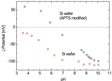
3.3.2 The ζ-Potential of APTS-functionalized Silicon Surface . . . . 37

3.3.3 Correction of Scattering Influence . . . . 38

1

3.3.4 The Structure of the Liquid Phase . . . . 39

3.4 Ion Distributions in Droplets . . . . 44

3.4.1 Counterion Distributions . . . . 44

3.4.2 Co-ion Distributions . . . . 45

3.5 Ion Distributions in Liquid Layers . . . . 50

3.5.1 Sample Preparation and Experiments . . . . 50

3.5.2 Optical Properties of Liquid Layers . . . . 50

3.5.3 Analysis of Substrate Fluorescence . . . . 51

3.5.4 The pH-Dependent Interfacial Charge of Si/APTS . . . . 53

3.6 Surface Functionalization by Polymer Brushes . . . . 56

3.6.1 Properties and Applications . . . . 56

3.6.2 Sample . . . . 56

3.6.3 Ellipsometry Experiments and Results . . . . 57

3.6.4 XSW Experiments and Results . . . . 58

4 XSW Analyses of Organic Semiconductors 62 4.1 Solution-Processed OLEDs . . . . 62

4.1.1 Samples . . . . 64

4.1.2 X-ray Resonance in Thin Layers . . . . 65

4.2 Measurement of the Sulfur Distribution . . . . 69

4.2.1 Accuracy of Sulfur Front Analysis . . . . 74

4.2.2 In-situ Analysis of the Crosslinking Process . . . . 76

4.2.3 Relative Excitation of the Sulfur Front . . . . 77

4.3 XSW Scans of Antimony Distributions . . . . 84

5 Conclusion and Outlook 89 5.1 Conclusion . . . . 89

5.2 Outlook . . . . 91

2.1 Ion Distribution Models . . . . 9

2.2 Streaming Current Measurement . . . . 12

2.3 Titration Reaction . . . . 13

2.4 Principle of XRF Excitation . . . . 14

2.5 Refraction of X-rays . . . . 16

2.6 Real and Imaginary Part of α _t , Reflectivity. . . . . 17

2.7 Refraction and Reflection . . . . 18

2.8 XSW field . . . . 19

2.9 Intensity Distribution I(z) . . . . 21

2.10 Fluorescence Simulation: Counterions . . . . 24

2.11 Fluorescence Simulation: Thin Marker Layers . . . . 25

2.12 Vertical Limitation of the XSW Field . . . . 27

2.13 coherent fraction . . . . 28

2.14 Principle of IR Ellipsometry . . . . 29

3.1 Setup of XSW Experiments . . . . 32

3.2 Single Spectra . . . . 34

3.3 ζ-Potential of Si/APTS . . . . 38

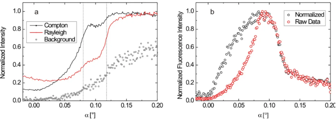
3.4 Compton and Rayleigh Scattering . . . . 39

3.5 Layers and Droplets . . . . 40

3.6 Reflectivity Signals of Layers and Droplets . . . . 41

3.7 Fluorescence Signals of Layers and Droplets . . . . 42

3.8 Br ⁻ Distribution on Functionalized Si . . . . 44

3.9 Distribution Models: Br/Fe . . . . 46

3.10 Fe ³⁺ / Fe(OH) ₃ Distribution on Functionalized Si . . . . 47

3.11 Estimation of Vertical Space Resolution . . . . 49

3.12 Beam Divergence . . . . 51

3

3.13 Substrate Fluorescence . . . . 52

3.14 Liquid Layer Samples . . . . 54

3.15 pH-Dependent Interfacial Charge . . . . 55

3.16 PAA Polymer Brushes . . . . 57

3.17 tan Ψ Spectrum . . . . 58

3.18 PAA Polymer Brushes . . . . 59

3.19 Polymer Brushes: Ion Distribution Measurements . . . . 60

4.1 PIX Crosslinking Process . . . . 64

4.2 Resonance of X-rays in Thin Layers . . . . 66

4.3 Overlap of XSW and X-ray resonance . . . . 68

4.4 Sequence of Spectra . . . . 69

4.5 Polymer Layers: Series A . . . . 71

4.6 Comparison of XSW and XRR Results . . . . 73

4.7 Fit of Shifted Front Models . . . . 75

4.8 Estimation of Sulfur Front Thickness . . . . 76

4.9 XSW Measurement during Heating Process . . . . 78

4.10 Fluorescence Excitation by XSW and Resonance . . . . 79

4.11 Polymer Layers: Series B . . . . 81

4.12 Relative Excitation of the Sulfur Front . . . . 83

4.13 Sb Containing Initiators . . . . 84

4.14 Fluorescence Spectrum of Sb-Containing Polymer . . . . 85

4.15 Sb Distribution (Propyl Containing Initiator) . . . . 86

4.16 Sb Distribution (Benzene Containing Initiator) . . . . 87

Introduction

1.1 Motivation

Interfaces between solids and liquids are omnipresent in nature and of great importance in many fields of biology, chemistry, medicine and research. Here, a multitude of pro- cesses which are important for life and health, like the transport of ions through cell membranes or the adsorption of bacteria and proteins on surfaces takes place [1, 2]. In general, solid/liquid interfaces are charged and many of the processes mentioned above are controlled or influenced by the electric interfacial potential [3, 4, 5]. Therefore, for a comprehensive understanding of interfaces and the related phenomena, knowledge of this so-called ζ-potential and the distribution of charges is necessary. Not only natural surfaces and their charge are of interest, but also the systematic modification of surfaces in order to control and influence the properties of interfaces and fluids [6, 7, 8, 9]. Such surface functionalization methods are of particular relevance for the development of microfluidic devices [10, 11].

However, possibilities of experimental analysis of the ζ-potential are restricted, mainly for two reasons: The presence of a liquid phase excludes all methods depending on vac- uum conditions; and the lateral extension of the ζ-potential, typically limited to few nanometres, requires a high spatial resolution. These restrictions are overcome by the experimental method described in this work, known as X-ray standing Waves (XSW) measurements. The distribution of ions adjacent to the surface, indicating the strength of the ζ-potential, is scanned vertically using XSW. X-ray standing waves are stationary electromagnetic interference fields generated by interference of an incoming an a reflected X-ray beam. The intensity of XSW-excited fluorescence as a function of the incident

5

angle enables the determination of element concentration profiles in the sample volume near the interface. X-ray standing waves have proven to be a well-suited tool for the study of nanometre-sized structures. The method is non-destructive, element sensitive and compatible to atmospheric pressure. The experiments performed are summarized below.

Surface Functionalizations

The experiments described in the third chapter are dedicated to the analysis of function- alized solid/liquid interfaces. First, the influence of a surface modification by functional groups on the interfacial charge and potential is studied. Results from the measurement of the streaming current yielding ζ-potential values and XSW scans of the diffuse ion layer are combined for the quantitative determination of the interfacial charge density.

A detailed discussion of the evaluation of XSW-excited fluorescence signals is included, explaining the correction of the effects which are induced by the morphology of the sample and the influence of scattering.

A further functionalization type is the coating of a surface with polymer brushes, which is of particular interest for the control of flows in microfluidic devices. Here, a combination of infrared ellipsometry and XSW scans was applied to determine the pH- dependent behavior of the brushes and their influence on wetting properties of the surface, respectively.

Polymer Layers

The second class of samples investigated in the framework of these studies are thin poly- mer layers containing an inhomogeneous distribution of sulfur ions. These samples are applied to the development of a novel fabrication process for organic light emitting diodes (OLEDs). Here, the main target of XSW experiments is the detection and characteriza- tion of a thin front of sulfur ions at low concentration. Herewith, a proposed polymer crosslinking mechanism is verified.

Although the actual topic of this work is the analysis of solid/liquid interfaces, the present sample type fits into the scope of the studies: In terms of reflection, refraction and absorption of X-rays, the polymer layers correspond to thin liquid films and can therefore regarded as solid-state solutions.

Furthermore, the initiation of the crosslinking process is observed in a series of ex-

periments recorded during the reaction. The investigation of element distribution within

the polymer layers not only provides insight into the sample structure and the reaction process, but also helps to understand the limitations of applicability of the experimental method: The vertical extension of the standing waves field is determined, which enables the estimation of the measuring range.

1.2 Historical Background

Shortly after the discovery of X-rays by R¨ ontgen in 1895, the value of this new type of radiation for analytical purposes was recognized. The diffraction experiments at crystals performed by M. v. Laue in 1912 were the first analyses of structures of atomic and molecular size taking advantage of X-ray interference. With the work of Moseley, who introduced the principles of element identification using X-ray fluorescence spectrometry (1913) and Compton, who first reported on total reflection of X-rays (1923), the founda- tions of the XSW method were laid [12, 13].

But only in 1971, Yoneda and Horiuchi combined these advantageous properties in the development of total-reflection X-ray fluorescence analysis (TXRF), which has be- come an established method in analytical chemistry [14, 15]. In the following years, instrumentation was developed and also first experiments using synchrotron radiation were performed [16, 17]. In the field of solid/liquid samples, XSW generated by total external and Bragg reflection have proven useful for the analysis of various interfacial processes and phenomena [18, 19], including the adsorption of ions, biofilms and proteins on surfaces [20, 21, 22, 23], the study of biologically relevant membranes [24, 25, 26, 27]

and surface reactivity [28, 29].

Compared to other X-ray related analytical techniques, XSW experiments are of rela-

tively limited application, mainly due to the special demands on beam quality which are

only practically met by synchrotron radiation.

Theoretical Background

2.1 Charged Solid/Liquid Interfaces

2.1.1 Ion Distribution Models

In general, interfaces between solids and solutions are charged. This is mainly due to dissociation of surface groups or to adsorption of ions from the solution onto a neutral surface [30, 31]. This charge and the resulting potential is of great relevance for many interfacial processes, but cannot be measured directly. Therefore, the distribution of ions at the interface, which is determined by the electric potential, is of particular interest for the analysis of solid/liquid interfaces.

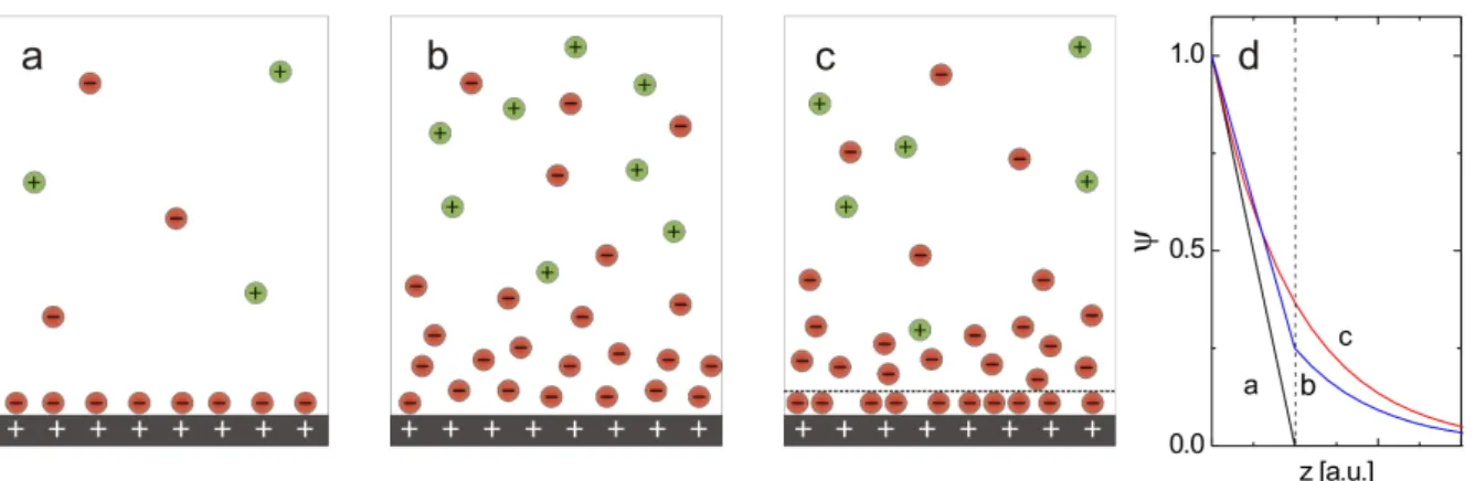
For the description of ion distributions, several models have been developed, of which three fundamental ones are shown in Figure 2.1. In the simplest model (a), proposed by Helmholtz [32], the charge of the solid surface is compensated by a layer of adsorbed (oppositely charged) counterions. Above this adsorbed layer, the solution is charge neu- tral. The second model (b), developed by Gouy and Chapman [33, 34], gives a more appropriate representation of the interface by taking into account the thermal motion of ions in the solution. This motion leads to the formation of a diffuse ion layer of expo- nentially decreasing counterion concentration, which shields the interfacial charge. With decreasing strength of the potential, the concentration of (equally charged) co-ions rises.

Considering co- and counterions, the diffuse ion layer is also referred to as electric double layer (EDL). In the bulk solution far from the interface, the concentration of both ion types is constant (bulk concentration). The Stern model (c) combines the features of the previously discussed models [35], consisting of an adsorbed layer and the diffuse layer of the Gouy-Chapman model. The thickness of the Stern layer determines the position of

8

Figure 2.1: Models for the distribution of ions adjacent to a charged interface according to Helmholtz (a), Gouy / Chapman (b) and Stern (c). The plot d schematically shows the relative potential strength ψ(z) for each case. The dashed line in c and d indicates the shear plane, separating adsorbed and mobile ions.

the shear plane which constitutes the boundary between mobile and immobilized ions.

For the analysis of the properties of charged solid/liquid interfaces with XSW, the diffuse ion layer is the most interesting part of the ion distribution. In the following discussion, a short derivation of the parameters which will be used for the characterization of the charge and the potential of the interface is given.

2.1.2 The Poisson-Boltzmann Equation

The Poisson equation is the fundamental equation for the description of the electric poten- tial of a distribution of charges. For the discussion of the characteristics of ion distributions in the electric potential above a surface, a charged plane is considered [36]. The potential ψ of the interfacial charge is determined by the Poisson equation

∇ ² ψ = −ρ

ε _r ε ₀ (2.1)

with the charge density ρ, vacuum permittivity ε ₀ and relative permittivity ε _r . The concentration of (oppositely charged) counterions within this potential is given by the Boltzmann equation

n _i = n ⁰ _i exp −c _i eψ kT

(2.2)

c _i is the valency of ion species i and n ⁰ _i is its bulk concentration far from the interface.

This concentration is not any more influenced by the ζ-potential and therefore is constant.

Considering all i ion species of the solution, the relation between the potential and the ion concentration is given by the Poisson-Boltzmann equation:

∇ ² ψ = −1 ε ₀ ε _r

X

i

n ⁰ _i c _i e exp −c _i eψ kT

. (2.3)

Assuming a small potential (eψ kT ), the Poisson-Boltzmann equation can be expanded:

∇ ² ψ = −1 ε ₀ ε _r

h X

i

c i en ⁰ _i − X

i

c ² _i e ² n ⁰ _i ψ/kT i

. (2.4)

Due to the neutrality of the bulk solution, the first sum has to be zero, which leads to the following linear approximation:

∇ ² ψ = h P 2 i e ² n ⁰ _i ε ₀ ε _r kT

i

ψ = κ ² ψ (2.5)

with the Debye-H¨ uckel parameter κ. Equation 2.5 is solved by exponentially decreasing potentials of the type ψ(z) = ψ ₀ exp(−κz ). The inverse of the Debye-H¨ uckel parameter is the Debye length L _D = 1/κ, which is a measure for the extension of the diffuse ion layer.

At z = L D , the concentration of counterions has decreased to 1/e ≈ 37%, the influence of the interfacial potential extends over a range of 3L _D to 4L _D .

However, in the case of most interesting charged interfaces, the condition for small potentials eψ kT is not fulfilled and the approximation discussed above cannot be made. Therefore, the Debye length of the counterion distribution above the analyzed interfaces will be determined experimentally applying X-ray standing waves.

2.1.3 The Interfacial Charge

The charge σ of the surface (per unit area) is balanced by the charge of the counterions of the diffuse layer:

σ = Z ∞

0

ρ(z)dz (2.6)

or, using the Poisson equation, σ = −

Z ∞

0

ε 0 ε r

d ² ψ

dz ² dz = ε 0 ε r

h dψ dz

i 0

∞ . (2.7)

In the bulk solution (z → ∞) the potential is constant, so the surface charge is given by σ = ε ₀ ε _r dψ ₀

dz (2.8)

with ψ ₀ = ψ(z = 0). The integration of the complete (one-dimensional) Poisson-Boltzmann equation yields:

dψ

dz = − 2κkT ce sinh

ceψ ₀ 2kT

. (2.9)

Inserting into equation 2.7 gives:

σ = − 2κε ₀ ε _r kT

ce sinh ceψ ₀ 2kT

, (2.10)

the so-called Grahame equation [30, 37]. Thus, knowing the values of ψ ₀ and L _D = 1/κ, the interfacial charge can be calculated. In the following, the experimental methods for the measurement of these parameters, summarized in Table 2.1, will be discussed.

Parameter Variable Unit Exp. Method ζ-Potential ψ ₀ mV Streaming Current

Debye Length L D nm XSW

Surface Charge σ mC/m ² -

Table 2.1: Parameters and experimental methods related to the characterization of

charged solid/liquid interfaces described in this work.

2.2 Streaming Current Measurements

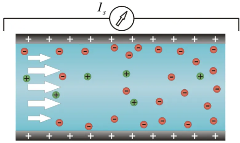
The ζ-potential ψ ₀ at the interface is determined by the electrokinetic measurement of the streaming current. Figure 2.2 schematically shows the experimental setup: An electrolyte solution is driven by external pressure through a channel or a capillary of the sample material. The flow also carries downstream the accumulated counterions of the diffuse layer, causing a net charge transport, the streaming current. As the concentration of counterions of the diffuse layer depends on the ζ-potential, the streaming current is related to ψ ₀ [31]:

I _s = εε ₀ ψ ₀ η

∆P

L A. (2.11)

where η is the viscosity of the electrolyte, ∆P/L the pressure gradient along the channel length and A the cross section of the channel or capillary.

Figure 2.2: Principle of the measurement of the streaming current. The flow in the channel or capillary moves the electric double layer, causing the streaming current I s .

2.2.1 Titration Reactions at Interfaces

The strength and polarity of an interfacial potential is determined by the interaction of the

charges of functional surface groups with the ions in the liquid phase. This interaction is

described by titration reactions. The pH dependent reaction equilibrium of two interfaces

bearing different functional groups A and B is considered. Equation 2.12 a describes the

protonation of molecule A in acidic solution, inducing a positive ζ-potential at low pH values. A negative surface charge is induced by the deprotonation of the hydroxyl groups of molecule B, represented by equation 2.12 b:

A + H ₃ O ⁺ * ) A-H ⁺ + H ₂ O (a) B-OH + OH ⁻ * ) B-O ⁻ + H ₂ O (b).

(2.12)

In the case of interfaces comprising several types of functional groups, the ζ-potential is given by the superimposition of the potentials induced by the single reactions. An example is plotted in Figure 2.3 (curve c). The pH value, for which positive and negative charges balance out each other, causing a neutral interface, is called the isoelectric point.

Figure 2.3: Titration curves for interfaces with different types surface groups determining

the charge. In curve a, the pH dependent ζ -potential induced by functional groups of type A,

being protonated in acidic solution, is plotted and curve b shows the potential corresponding

to a deprotonation of hydroxyl groups (B) with rising pH. The potential of an interface bearing

functional groups of both types is represented by curve c. At pH 7, the isoelectric point (ψ c = 0)

of the interface described by curve c is passed.

2.3 Principles of X-ray Standing Waves

2.3.1 X-ray Fluorescence

X-rays are electromagnetic waves of short wavelength, following the ultraviolet range in the electromagnetic spectrum. Their energy, in the present work generally given in kiloelectronvolts (keV), is related to the wavelength λ and can be calculated by

E = hν

c = 1.2397

λ[nm] keV. (2.13)

X-rays can be produced in the form of primary and secondary radiation. For the gen- eration of primary X-rays, charged particles (electrons or positrons), are accelerated in electric fields (as in X-ray tubes) or magnetic fields (bending magnets or insertion devices of synchrotrons). Secondary X-rays are emitted by the transition of an electron from one energy level of an atom to a lower one. The principle of this process is shown in Figure 2.4.

Figure 2.4: Left: Principle of X-ray fluorescence excitation. An incoming X-ray photon (1) expels an electron of an inner shell of the atom (2). An electron from a higher energy level moves, filling the vacancy (3). The energy difference between the two shells is balanced by the fluorescent emission of a photon (4). In the picture, the excitation of the Kα line of carbon is shown as an example. Right: Kα and Kβ electron transitions.

Referring to Figure 2.4, the basic principle of X-ray fluorescence spectrometry is ex-

plained as follows: A primary X-ray photon of wavelength λ = c/ν hits an electron of

one of the inner shells and, if the photon energy hν is higher than its binding energy, removes it. To restore an energetically favorable state, a second electron from a higher energy level moves and occupies the vacant position. The energy difference between the two shells is compensated by the fluorescent emission of a (secondary) photon. Its energy is approximately determined by the principal quantum numbers n ₁ and n ₂ of the two shells and by the atomic number Z of the irradiated element:

E _ph = Z ² e ⁴ m ₀ 32π ² ε ² ₀ ¯ h ²

1 n ² ₂ − 1

n ² ₁

. (2.14)

In the example of the carbon Kα transition shown in Figure 2.4, the values are Z = 6, n 1 = 1 and n 2 = 2. By this transition, a photon of E ph = 0.277 keV is emitted. As a con- sequence of this, elements can be identified by the spectrum of their characteristic X-ray fluorescent emission. A more detailed introduction into X-ray fluorescence spectrometry can be found in the references [38] and [39].

2.3.2 Reflection and Refraction of X-rays

The basic principles and conditions for the generation of X-ray standing waves fields will be discussed below [41, 42]. An X-ray beam passing the interface between two media of different electron density is considered. The deflection of the incident beam, schematically shown in Figure 2.5, is described by Snell’s law of refraction

n ₁ cos α _i = n ₂ cos α _t (2.15)

where α _i and α _t are the angles of the incident and transmitted beam relative to the surface, respectively. For grazing incidence X-rays, angles are measured relative to the surface instead of to its normal, as it is usually done in optics.

The (complex) refractive indices of the media n ₁ and n ₂ are defined by

n = 1 − δ + iβ (2.16)

with the imaginary unit ¹ i = √

−1. The real part δ is called the decrement and describes the dispersion of beam. Attenuation of the radiation in the medium is given by the

1

Alternative notation: n = 1 − δ − iβ, in this case the sign of the complex term changes.

Figure 2.5: Refraction of an X-ray beam passing an interface between two media of different refractive indices. Here, medium 1 is optically thicker (n 1 > n 2 ).

imaginary part β. The two parameters depend on material properties of the irradiated media and on the wavelength λ of incident radiation

δ = λ ²

2π r _e ρ _e (2.17)

β = λ

4π µ (2.18)

with the classical electron radius r _e = e ² /(4πε ₀ m _e c ² ) = 2.814 · 10 ⁻¹⁴ nm, electron density ρ e = N A Zρ/A (N A : Avogadro’s number, A: atomic mass) and the absorption coefficient µ. For X-rays, the parameters δ and β normally are of the order of magnitude 10 ⁻⁶ and 10 ⁻⁹ , respectively. The real part of the refractive index in media is smaller than in vacuum (n < n _vac = 1), thus X-rays hitting a vacuum/medium interface under grazing incidence are deflected towards the interface. A critical incident angle α _c exists, where the angle of the transmitted beam α _t is zero. If the electron density of medium 1 can be neglected, cos α c = n 2 applies (from equations 2.15 and 2.16) and for the small incident angles used in XSW experiments, the following approximation can be used

cos α _c ≈ 1 − α _c ²

2 (2.19)

from which (considering only the dispersion given by δ) the critical angle can be calculated α _c = √

2δ. (2.20)

At the interface of two media of both non-negligible electron density (example shown in

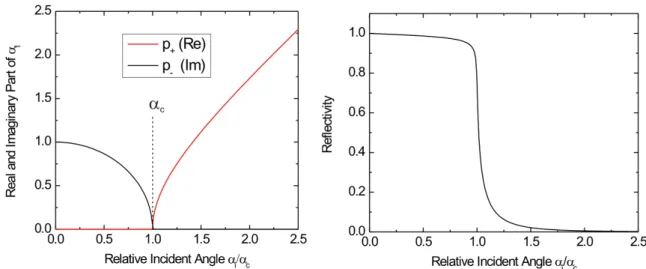
Figure 2.6: Left: Real and imaginary part of the transmission angle α _t . For α < α _c , incident radiation is reflected, α t is imaginary. For incident angles exceeding the critical angle, α t becomes real and the radiation penetrates into the medium. In the right graph, the calculated reflectivity curve of a Si surface is plotted. The x-axis of both plots is normalized to the critical angle α c .

Figure 2.7), dispersion is determined by the difference of the two decrements δ = δ ₂ − δ ₁ . Using equations 2.15 and 2.16, the transmission angle α _t can be approximated by

α t = q

α ² _i − 2δ + 2iβ (2.21)

The real and the imaginary part of the transmission angle α _t = p ₊ + ip ₋ is defined by the equation

p ² _+/− = 1 2

hq

(α ² _i − α ² _c ) ² + 4β ² ± (α ² _i − α ² _c ) i

(2.22)

The two components are plotted in Figure 2.6. For α i α c , the real part of α t asymp- totically approximates α _i . Below the critical angle, equation 2.15 yields no real value for α _t . The transmission angle is complex and the incident wave does not penetrate into the medium. Instead, radiation is totally reflected at the interface [13, 40]. The intensity of the reflected beam is calculated according to the Fresnel formulas and is given by

R F (α i ) = (α _i − p ₊ ) ² + p ² ₋

(α _i + p ₊ ) ² + p ² ₋ . (2.23)

The left graph of Figure 2.6 gives an example of an ideal reflectivity curve calculated for a silicon substrate irradiated by X-rays of 15.5 keV energy. The intensity of the reflected beam is affected by the ratio β/δ and by the roughness of the reflecting surface. Different approaches exist to take into account roughness [41, 43], in the calculations discussed in this work it is done by multiplication of R _F with a Debye-Waller factor

r _DW = e

2z σ2 rms

2

(2.24)

with the vertical wave vector transfer q _z = 4π sin α/λ, σ _rms is the root-mean-square roughness.

Figure 2.7: Refraction and reflection of an X-ray beam at a system of two interfaces. The beam, coming from vacuum (δ 0 = 0), hits the interface I 01 under an incident angle α ⁰¹ _i > √

2δ 1

and is transmitted into medium 1 under the angle α ⁰¹ _t . The new incident angle α ¹² _i inside medium 1 is smaller than the critical angle of the interface between medium 1 and medium 2 (α ¹² _i < p

2(δ ₂ − δ ₁ ) ), thus total reflection occurs at I ₁₂ .

Figure 2.7 demonstrates the refraction and reflection of X-rays at interfaces in the case of a beam path through a layered sample of different media. In the example, the parameters of radiation and sample material are chosen in such way that the beam is transmitted into medium 1 and then reflected at the interface between the media 1 and 2.

The reflected beam is again refracted at the surface of medium 1 and leaves the sample

under the exit angle α ¹⁰ _t = α ⁰¹ _i .

2.3.3 The X-ray Standing Waves Field

When a beam of monochromatic, coherent and parallel X-rays hits a plane surface with α _i < α _c , the incident and reflected part of the radiation interfere in the overlap region, generating the X-ray standing waves field. X-ray standing waves are stationary electro- magnetic fields of alternating intensity minima (nodes) and maxima (antinodes) parallel to the reflecting surface. Figure 2.8 schematically shows the geometrical parameters and the vertical intensity distribution of an XSW field.

Figure 2.8: Schematic plot of an XSW field and its vertical intensity distribution I _α (z). The relation of wavelength λ to the distance a between two maxima is explained in the text.

The intensity of the field is a function of the incident angle α and the vertical distance z from the reflecting surface. In the following, the incident angle is referred to as α.

I(α, z) = I ₀ h

1 + R(α) + 2 p

R(α) cos(2πz/a − φ(α)) i

. (2.25)

The intensity of incoming beam is assumed to be constant. For the reflectivity R ≤ 1 applies, as shown in Figure 2.6. The third term of equation 2.25 describes the interfer- ence of the incident and the reflected wave. The argument of the cosine includes the path difference of incoming and reflected wave 2πz/a and the phase shift φ(α). Under total re- flection conditions, the interference term takes values between +2 p

R(α) and −2 p R(α).

Depending on α and z, the summation of all three terms leads to the oscillation of intensity

I _α (z) between 0 and ≤ 4 · I ₀ . The phase shift φ(α) is given by

φ(α) = arccos[2(α/α _c ) ² − 1]. (2.26)

The phase shift has its maximal value of π at α = 0, decreasing to zero at α = α _c . The distance a between two field nodes or antinodes is

a = λ

2 sin α (2.27)

This distance decreases with increasing incident angle, its minimal value a _min is reached at the critical angle

a _min = λ

2 sin α _c (2.28)

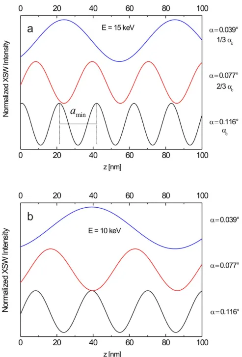
Using radiation of constant wavelength, the vertical position of nodes and antinodes is changed by the variation of the incident angle. The increase of α shifts nodes and antin- odes towards the surface and causes a compression of the XSW field. Figure 2.9 shows the vertical intensity distribution of some XSW fields calculated for X-rays of different energy and incident angle, reflected at a silicon surface. The parameters of these field are given in Table 2.2. The parameters of the fields are summarized in Table 2.2. The energy values of 10 and 15 keV were chosen according to the experiments, which will be discussed in the following chapters. Most measurements have been carried out using radiation of 15 - 15.5 keV, the corresponding field is shown in diagram a of Figure 2.9.

The lowest energy applied to the generation of standing waves was 10 keV, the intensity

distribution is displayed in plot b. Curves of same color represent fields of identical angle

of incidence, so the dependency of the period a of the fields from λ and α can clearly be

seen: The increase of energy, corresponding to a decrease of wavelength λ, reduces the

distance between the respective nodes of the field. Comparing the curves plotted blue, red

and black, which corresponds to incident angles of α = 0.039 ^◦ , α = 0.077 ^◦ and α = 0.116 ^◦ ,

respectively, the compression of standing waves is obvious. For E = 15 keV, the first two

chosen angles correspond to one third (blue) and two thirds of α _c (red); the black curve

shows the maximal compression for the field at the critical angle. Here, the period of the

standing waves field takes its minimal value a min . The vertical accuracy of XSW scans of

elemental distributions, which will be explained in the next section, largely depends on

this quantity.

Figure 2.9: Vertical intensity distribution of XSW fields on a Si reflector for different energies and incident angles. Signals were calculated for an X-ray energy of 15 keV (a) and 10 keV (b).

Incident angles are 0.039 ^◦ (blue), 0.077 ^◦ (red) and 0.116 ^◦ (black). For E = 15 keV, the chosen

angles correspond to 1/3α c , 2/3α c and α c , respectively.

I(z) graph α[ ^◦ ] α/α c (E = 15 keV) a 15

[nm] a 10

[nm]

blue 0.039 1/3 61.1 91.7

red 0.077 2/3 31.1 46.5

black 0.116 1 20.6 30.9

Table 2.2: Parameters of the XSW fields plotted in Figure 2.9.

2.3.4 Excitation of Marker Fluorescence

Now, a distribution of atoms or ions near on a surface or near an interface will be con- sidered. This surface or interface is irradiated by a grazing-incidence X-ray beam and a standing waves field is produced, which overlaps the element distribution. Consequently, the fluorescence of these so-called markers is excited by the intensity maxima (antinodes) of the XSW field. Compared to conventional fluorescence excitation which is done us- ing only the intensity of incident radiation I 0 , the interference of incident and reflected beam in the XSW field according to equation 2.25 significantly amplifies the excitation of fluorescence. Thus, the detection limit of an analyte excited to fluorescence by XSW is considerably lower than in the case of conventional XRF analysis.

With angular resolved measurements of XSW-excited fluorescence, distribution of ele- ments can be determined. As already mentioned, the position of XSW field maxima de- pends on the incident angle and the wavelength of the radiation. Usually, the wavelength is adjusted to a constant value for XSW experiments, so the variation of the incident angle is used to move the antinodes of the field through the marker distribution. For a given angle interval, typically ranging from α = 0 to α ≈ 1.5 · α _c , the fluorescence of the atoms or ions within the XSW field is recorded, whereas the incident angle is increased stepwise. In doing so, the distribution of elements is scanned vertically.

The measured fluorescence signal is the product of the intensity of the XSW field I(z) and the marker concentration at the respective height over the surface. The fluorescent photons from the entire vertical range of the sample volume are collected simultaneously, so the relative intensity of an XSW-excited marker distribution D(z) is given by the integral

I(α) = Z z

0

I(α, z) · D(z)dz. (2.29)

Assuming a typical value for the beam height of ca. 100 µm and a wavelength on the

order of magnitude of 0.1 nm, several hundreds maxima and minima are expected within the XSW field. However, the interference field does not fill the entire intersection volume of incoming and reflected beam, as in the idealized case shown in Figure 2.8, but extends only to a limited distance from the reflecting surface, which is indicated by the upper integration limit z _max [44]. This parameter determines the vertical extension of the XSW field, which is limited by the finite longitudinal coherence length of incoming and reflected radiation.

Later on, this issue will be analyzed in more detail and different factors influencing the vertical extension of the XSW field will be discussed. Furthermore, the fading of the interference field by the decrease of node/antinode contrast as a function of distance to the surface will be examined. Above z _max , the interference field is replaced by the unmodulated overlap of incoming and reflected beam. Thus, the fluorescence of any markers situated in this region is excited by

I _z>z

(α) = I ₀

1 + R(α)

(2.30)

and may, for sufficient marker concentrations and α ≤ α c contribute to the XSW-excited signal in the form of an intensity offset.

Depending on the volume and composition of the sample material covering the re- flecting surface, scattered radiation may cause a further contribution to the excitation of marker fluorescence. Especially, when the interesting markers are embedded in a liquid, as for example ions in aqueous solutions, this effect must be taken into account. The correction of this influence will be discussed in the experimental section.

2.3.5 Simulation of Fluorescence Signals

Different types of elemental distributions have been analyzed in the context of these

studies. The most important ones are exponentially decreasing concentration profiles of

counterions and thin marker layers at a distance of up to 130 nm from the surface. To

introduce the characteristic features of the corresponding fluorescence signals, some inten-

sity curves which are expected for these distributions are calculated and will be discussed

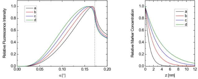
in the following. Figure 2.10 shows some typical counterion signals which were calculated

using the Gouy-Chapman model with varying Debye length. Simulations were done for

an X-ray energy of 10 keV, here the minimal period of the XSW field a min of ca. 20 nm

is significantly larger than the vertical extension of the marker distribution. Correspond-

ingly, only the lowest XSW antinode overlaps with the ions and only one fluorescence maximum appears. Comparing the curves a - d, the relation between the extension of the diffuse ion layer (given by L _D ) and the shape of the maximum in the related fluorescence signal is demonstrated. A scan of the distribution profile a, representing a highly com- pressed diffuse layer (L _D = 1 nm), leads to a very sharp fluorescence maximum, which is located at the critical angle. This is explained as follows: Only shortly before α _c , the antinode reaches the region of significant ion concentration, thus here the largest part of fluorescence is excited before reflectivity drops off. In the case of a broad ion distribution, as shown in the profile d (L _D = 4 nm), the wave overlaps at a given angle with a much higher marker concentration compared to case a. Thus, also the resulting fluorescence maximum is broader and its angle position slightly shifted towards smaller values.

Figure 2.10: Calculated examples of XSW-excited fluorescence intensity curves (left) with the corresponding marker distribution profiles (right). Curves a - d represent an exponentially decaying marker concentration, which is typical for counterion distributions. The curves were calculated for a Si substrate and 10 keV X-ray energy, the critical angle is marked by a dashed line.

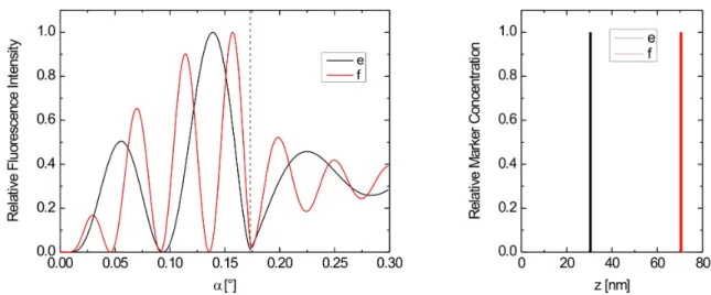
Results like those shown in Figure 2.11 are expected for XSW scans of thin marker

layers at a distance of several XSW field periods above the surface. Here, the fluorescence

signal oscillates, which indicates the transition of XSW maxima through the layer. Each

antinode of the field passing the layer generates one fluorescence maximum. Here, the

distance between the reflecting surface and the marker layer is larger than the shortest

possible oscillation period a _min of the standing waves field, so for m maxima before the

critical angle, the position of the layer can be estimated to m · a _min ≤ z < (m + 1) · a _min (cf. equation 2.28). For the marker layer at a distance of 30 nm above the surface, two fluorescence maxima appear. A shift of the layer to z = 70 nm increases this number to four.

Figure 2.11: Calculated examples of XSW-excited fluorescence intensity curves (left) with the corresponding marker distribution profiles (right). The signal expected for a thin marker layer is plotted in the curves e and f for different layer positions. The curves were calculated for a Si substrate and 10 keV X-ray energy, the critical angle is marked by a dashed line.

Generally, it can be noticed that fluorescence detected near the critical angle originates from markers near the surface (z < a _min ), whereas markers far from the surface (z a _min ) contribute to the signal measured at small angles (α < α _c /2).

For the evaluation of XSW-excited fluorescence signals, an intensity curve I(α) is cal-

culated and fitted to the measured data. As mentioned above, the fluorescence intensity

is the integrated product of the intensity of the XSW field I(α, z) and the element distri-

bution D(z). With the parameters of the sample (refractive indices of the components of

the sample) and of the beam (wavelength, incident angle, critical angle), also the XSW

field is known. From sample preparation, often a certain distribution of markers can be

expected or, considering the criteria explained above, can be deduced from the measured

signal. So, a first probable distribution profile D(z) is proposed. Then, the simulation

of the XSW-excited fluorescence signal according to equation 2.29 is calculated using the

chosen distribution model. This simulation procedure is repeated, varying the parameters

of D(z) in order to optimize the agreement between measured and calculated data. The model, for which optimal fit quality is achieved, can be regarded as representing the actual marker distribution at the interface of the analyzed sample.

2.3.6 Vertical Limitation of the XSW Field

As every experimental method, XSW scans have their limitations of applicability. The following discussion explains the restriction of the vertical range of measurement, which is already suggested by the upper integration limit z max used in equation 2.29.

Until now, an ideal XSW field has been considered, where nodes and antinodes fill the entire intersection volume of incoming and reflected beam. However, in experiments it has been found that this does not match real conditions. This is mainly caused by the finite longitudinal coherence of the radiation which generates the field. Figure 2.12 demonstrates the realistic case, where the beams interfere only in the lower part of the overlap triangle. This effect has two main reasons: the longitudinal coherence length of the incident radiation is finite and the fraction of coherent radiation of the incoming beam is reduced by scattering processes inside the sample material. The longitudinal coherence length of an X-ray beam is defined as the distance, that two parallel wave trains starting from the same point have to propagate until their respective maxima and minima overlap [29]. Thus, the longitudinal coherence length ξ _l depends on the wavelength and the wavelength difference between the two wave trains ∆λ and is given by

ξ _l = λ 2

λ

∆λ . (2.31)

In practice, the longitudinal coherence length of the X-rays irradiating the sample is determined by the quality of the monochromator applied to the X-ray beam. A real monochromator emits a narrow bandwidth of wavelengths. The wavelength-dependent intensity distribution of the monochromatized beam is generally described by a normal distribution. The quality of a monochromator is defined by the full width at half maximum (FWHM) ∆λ of the intensity distribution. Typical values for single-crystal monochroma- tors are ∆λ/λ ≤ 10 ⁻⁴ . The wavelength difference ∆λ induces a variation ∆a of the field period given in equation 2.27. Thus, the nodes and antinodes of XSW fields generated by beams of different wavelengths are shifted vertically, which reduces the contrast of the interference field.

The effect of finite beam monochromaticity is significant at positions far from the

Figure 2.12: Vertical limitation of the XSW field caused by the finite coherence length of incident radiation. The dimensions are not shown in true scale.

interface and plays a role for media of very low electron density such as air or vacuum.

It has been studied by von Bohlen et al. by XSW measurements of nanoparticles of up to 250 nm diameter on a silicon surface [44, 45]. From the comparison of measured and calculated fluorescence curves for particles of different size, it was observed that particles of a diameter of 100 nm and more were not any more completely irradiated by the field.

From the deviation between calculated and experimental data, a vertical extension of the XSW field of z ≥ 83 nm was deduced.

However, the finiteness of longitudinal coherence length cannot be not the only reason for the vertical limitation of the XSW field, as in experiments with solid/liquid interfaces very different values for z max have been found for nearly identical combinations of X-ray energy and substrate material. Thus, it seems likely that also the solution containing the marker distribution has a great effect on the range of interference.

In experiments analyzing marker distributions embedded in liquid and polymer layers on the surface it has been observed that z _max of the best-fit distribution models decreases with increasing volume of the sample material covering the reflecting surface. Thus, the conclusion can be drawn that, for the transition of the beam through a medium of non-negligible electron density, the loss of coherence is mainly caused by scattering and absorption of incident photons. This can be understood using the example of an idealized case.

Considering a beam of originally coherent radiation, scattering and absorption pro-

cesses reduce the fraction of coherent photons until all coherence is lost. For the cal-

Figure 2.13: Principle of the vertical limitation of the XSW field due to a scattering-induced loss of coherence. For the two beams 1 and 2, interfering at the point P, a linear decrease of the coherent fraction is assumed. The maximal path length of coherent radiation l _max inside the medium determines the upper limit z max of the interference range. Right: the fractions of coherent radiation C ₁ and C ₂ for the beams 1 and 2 are plotted as a function z. The shaded area indicates the relative intensity of interference, determined by the product of C 1 and C 2 .

culation of h _XSW and the coherent fraction, the scattering and absorption properties of the respective sample must be known. For the general discussion of the effect, a simple linear decrease of the coherent photon fraction C is assumed. The geometry of the beam path is shown in Figure 2.13: The coherence of the incident beam 1, which passes a layer of thickness d is completely lost after a certain path length indicated l _max . The highest point, where the second beam 2 can interfere with beam 1 is marked P, its vertical position determines z _max . The vertical extension of the field h _XSW is given by

h _XSW = l _max · sin α − d. (2.32)

In the right part of Figure 2.13, the relative intensity of interfering (coherent) wave trains is plotted as a function of the distance z from the reflecting interface. The photons of beam 1 are moving towards the interface (blue dashed line) and reflected at z = 0. After reflection, the propagation direction is towards the sample surface at z = d (solid line).

Beam 2, hitting the the sample surface at a horizontal offset ∆x, has a shorter path length

(red solid line) to the point of interference P inside the medium. Consequently, the higher

P is located, the more coherence is lost in beam 1 and preserved in beam 2. The product

of C ₁ and C ₂ (marked grey), giving the relative intensity of the interference, is zero for

z > z _max .

2.4 Infrared Spectroscopic Ellipsometry

A further experimental method which is used in combination with XSW experiments for the characterization of the properties of surface functionalizations is infrared spectroscopic ellipsometry (IRSE) [46, 47]. Figure 2.14 schematically shows the principle of ellipsometric measurements: Linearly polarized light is reflected at a surface. By the reflection, a phase shift ∆ between the s- and p-polarized components is induced, thus the reflected radiation is polarized elliptically.

Figure 2.14: Principle of ellipsometry measurements.

The reflected radiation can be described by the amplitude ratio ρ of its (orthogonally polarized) components r _s and r _p

ρ = r _p

r _s = tan Ψe ^i∆ . (2.33)

The absolute ratio of the amplitudes of the two components is given by tan Ψ = |r _p |

|r _s | . (2.34)

Incoming infrared light excites different vibration modi of the chemical bonds in the sur-

face molecules, which causes polarization-dependent absorption of the reflected radiation

at characteristic wavenumbers, the so-called vibrational bands. By measurement of am-

plitude ratio of the two components of reflected intensity as function of the wavenumber

(tan Ψ spectrum), these vibrational bands are detected, which enables the identification

of chemical bonds and the state of surface molecules [48, 49]. In particular, the study

of protonation and deprotonation processes of functional surface groups, changing the

interfacial charge, is of interest for the present applications.

Summary of Chapter 2

In this chapter, the theoretical background of the experiments performed in the frame- work of this thesis was presented. First, some basic principles of the distribution of ions in the electric potential of a charged solid/liquid interface were introduced. The experimen- tal methods for the measurement of the parameters characterizing the interfacial charge and potential were discussed, focusing on the X-ray standing waves field. The genera- tion and the typical dimensions of the interference field, the evaluation of XSW-excited fluorescence signals and factors limiting the applicability of the method were explained.

The experimental analysis of different types of ion distributions by standing waves will

be presented in the following chapter.

XSW Analyses of Solid/Liquid Interfaces

3.1 Experimental Setup

The typical components of the setup of XSW experiments are shown in Figure 3.1. For angular resolved XSW experiments, bright X-rays of high coherence and of low divergence are needed. To achieve this, synchrotron radiation is required. X-ray are generated, when charged particles (electrons or positrons) is accelerated in a magnetic field. This is done in the bending magnets, which are used to force the electrons into a circular orbit of the storage ring or in the so-called insertion devices, which are specially designed for this purpose. Common insertion devices are wigglers or undulators, consisting of a row of alternating magnetic fields. Electrons passing these devices follow a wavy trajectory, this successional acceleration of charges induces the emission of a cone of synchrotron light. Synchrotron radiation is emitted tangentially to the storage ring and led to the experimental stations by the so-called beamlines.

Any bending magnet and insertion device emits a continuous spectrum of radiation, so the wavelength of synchrotron radiation extends from the infrared to the hard X- ray range. At the so-called critical energy, the intensity of emitted radiation is near its maximum. As discussed in the previous chapter, XSW fields can only be produced using monochromatic radiation. For this purpose, the polychromatic (“white”) beam is monochromatized, which in the hard X-ray range typically is done by double Bragg reflection at single crystals or at multilayer mirrors. The desired wavelength is selected by adjustment of the angle between mirror surface and the axis of the beam.

31

The photon energy used for the described experiments ranged between 10 and 17.48 keV. On adjusting beam energy, often a compromise has to be found between the respec- tive advantages and disadvantages of marker excitation by high and by low energy. With X-rays of high energy, more elements can be excited to fluorescence. However, in the case of the beamlines where measurements have been carried out, the intensity of the beam is higher at lower energy values, which are nearer the critical energy. So, for example, at the SAW beamlines at DELTA (E _crit = 7.9 keV), the increase of energy of monochromatized radiation from 10 keV to 15 keV considerably reduces the brightness of the beam.

Figure 3.1: Principle of the experimental setup of XSW experiments. Radiation is generated by radial acceleration of electrons or positrons in the bending magnets or insertion devices (ID) of the storage ring. The X-ray beam is configured by the X-ray optics and irradiates the sample under grazing incidence. A goniometer is applied for the adjustment of the incident angle, a reflectivity detector (RD) records the intensity of the reflected beam. The position of the XSW field is marked by red lines. The fluorescence detector (FD) collects the photons excited in the XSW field (blue).

A system of slits confines the horizontal and vertical extension of the beam in order to limit the irradiated area (footprint of the beam) to the sample surface. The adjustment of the incident angle is done by rotation of the sample, which is placed on a goniometer capable of moving angular steps on the order of 0.001 ^◦ with high repeatability.

Parallel to marker fluorescence, the intensity of the reflected beam is recorded, which

is done in the present experiments using ionization chambers, scintillation counters and

photodiodes. The measurement of reflectivity is applied to the exact positioning of the

sample in the rotation center of the goniometer. Furthermore, reflectivity curves contain

information about the structure of the sample, as for example roughness, evenness and

the thickness of layers on the substrate.

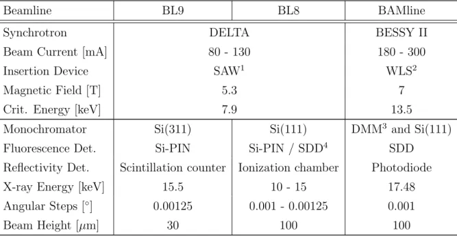
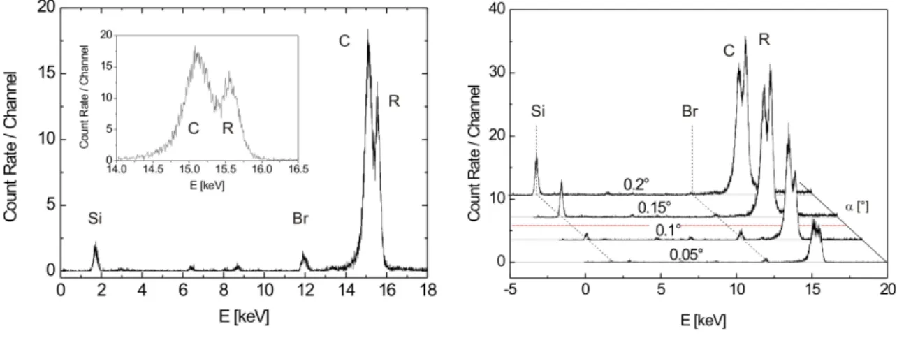
The essential information of XSW experiments is the angular dependent intensity of fluorescence emitted from the marker atoms or ions. It is measured by a semiconductor detector which is mounted perpendicular to the sample. One spectrum is recorded per angle step. The use of this energy-dispersive detector type enables the element-sensitive measurement of fluorescence. The experimental procedure is controlled by a computer and consists of moving of the sample, recording reflectivity and fluorescence and process- ing the fluorescence signal via an MCA (Multichannel Analyzer). Table 3.1 summarizes the technical parameters and experimental settings of the beamlines employed for the measurements described in this work. Experiments were performed at the synchrotron radiation facilities DELTA (TU Dortmund, Germany) and BESSY II (Helmholtz-Zentrum Berlin f¨ ur Materialien und Energie, Germany).

Beamline BL9 BL8 BAMline

Synchrotron DELTA BESSY II

Beam Current [mA] 80 - 130 180 - 300

Insertion Device SAW ¹ WLS ²

Magnetic Field [T] 5.3 7

Crit. Energy [keV] 7.9 13.5

Monochromator Si(311) Si(111) DMM ³ and Si(111)

Fluorescence Det. Si-PIN Si-PIN / SDD ⁴ SDD

Reflectivity Det. Scintillation counter Ionization chamber Photodiode

X-ray Energy [keV] 15.5 10 - 15 17.48

Angular Steps [ ^◦ ] 0.00125 0.001 - 0.00125 0.001

Beam Height [µm] 30 100 100

Table 3.1: Parameters of the beamlines used for the XSW experiments described in this work.

1

Superconducting Asymmetric Wiggler

2

Wavelength Shifter

3

Double Multilayer Monochromator

4

Silicon Drift Detector

3.2 Fluorescence Excitation Using Total X-ray Re- flection

The grazing incidence geometry of XSW experiments involves particular advantages com- pared to classical X-ray fluorescence analysis (XRF). Under total reflection conditions, the incoming beam practically does not penetrate into the substrate carrying the sample, which causes an effective reduction of spectral noise and matrix effects. Furthermore, interference of incoming and reflected radiation significantly enhances the excitation of the sample atoms. This way, under optimal experimental conditions, a very low limit of detection (LOD) in the sub-nanogram range is achieved [16, 17].

Figure 3.2: Left: Fluorescence spectrum excited under grazing incidence (α ≈ α _c , E = 15.5 keV). The first peak (Si Kα line) originates from the radiation penetrating into the substrate, the two peaks at the high-energy end of the spectrum (highlighted in the inset plot) are caused by scattering. Right: Development of signal intensity as function of the incident angle. The rise of scattering intensity, noise level and substrate fluorescence for α > α _c can clearly be seen, whereas marker fluorescence vanishes. Only for α < α c , the fluorescence marker peak (Br Kα) can clearly be separated from the spectral background . The red line indicates the position of the critical angle α _c = 0.12 ^◦ .

The typical properties of XSW-excited fluorescence signals will be discussed referring

to the examples of Figure 3.2. The spectrum plotted on the left is recorded close to

the critical angle, where reflectivity and with it the contrast of the XSW field begins

to decrease. The marker element of the solution is bromine, the characteristic Kα line

(E = 11.92 keV) can easily be identified. The spectrum is recorded near the critical angle, thus fluorescence of the silicon substrate emerges (Si Kα, E = 1.74 keV), indicating a partial penetration of the beam into the substrate. The spectrum is dominated by the peaks of elastic (Rayleigh) and inelastic (Compton) scattering. In the right part of Figure 3.2, a series of successively recorded spectra from an XSW scan are plotted. The development of the fluorescence intensities of marker and substrate as well as Compton and Rayleigh scattering can be observed. Bromine again is the analyte, the signal is clearly separated from the background in the first two spectra. The rise of intensity indicates a maximum of bromine concentration at the reflecting interface. For α > α _c , the peak disappears in the spectral noise. The intensity of substrate fluorescence behaves inversely, the peak emerges at the end of the total-reflection range and remains at a constant level for α > α _c .

Scattering intensity strongly rises around the critical angle, whereas the Compton peak prevails for α < α _c and Rayleigh intensity for α > α _c . The weak fluorescence lines between 6.4 and 8.6 keV (Kα lines of Fe, Cu and Ni) are induced by the excitation of the material of the components of the experimental setup by scattered photons.

3.3 Functionalization by Surface Groups

The first samples analyzed in the framework of the presented studies are surfaces coated by functional groups. The purpose of this modification is the variation of the interfacial charge. The interfacial potential is analyzed by the measurement of the extension of the diffuse ion layer using X-ray standing waves. These experiments are done in combina- tion with streaming current measurements. Besides the evaluation of fluorescence data, a discussion of the characterization of the structure of the liquid phase covering the sur- face with X-rays fluorescence and reflectivity is given, which is important for the correct interpretation of the measured curves.

In other studies, X-ray reflectivity has also been used to investigate the distribution of particles and charges near the solid/liquid interface [50, 51]. However, this technique is not element-sensitive and could therefore not be applied to the present task.

3.3.1 Sample Composition and Preparation

In these experiments, samples were silicon wafers modified by aminosilane surface groups.

By means of this sample, the pH-dependent influence of a surface functionalization on

the charge and ζ-potential of the interface was studied [52]. Substrates were prepared by immersion of silicon wafers (size ca. 4 cm ² ) in acetone solution containing 2-3%

aminopropyl-triethoxysilane (APTS) for 10 minutes and subsequent toluene rinsing. In microfluidics, APTS is used to link other functional groups to an oxidized silicon surface [53], in the present experiment the amino group is applied to the modification of the surface charge. It is determined by the ratio of protonated amino groups (functionalization) and silanol groups (native silicon oxide layer) and given by the following equations:

NH ⁺ ₃ + H 2 O ←→ NH 2 + H 3 O ⁺ (a) SiOH + OH ⁻ ←→ SiO ⁻ + H ₂ O. (b)

(3.1)

The liquid phase covering the wafers consisted of KBr and Fe(NO) ₃ solutions of different pH values. Br ⁻ and Fe ³⁺ ions were applied to the measurement of anion and cation distributions, respectively. The marker concentration was 10 mg/l in each case, the pH value determining the reaction equilibrium was adjusted by titration with HNO ₃ and NaOH solution. Under acidic conditions, measurements were performed at pH 2.8 and 5.7, in the alkaline case at pH = 10.

Differing from XSW experiments with solid structures as particles or layer systems, in the case of the analysis of solid/liquid interfaces the problem of the stability of the sample during measurements arises. The strong scattering of X-rays in water allows an only very small volume of the liquid phase on the reflector, otherwise the high spectral background and the contribution of fluorescence originating from the unmodulated field would inhibit the identification of evaluation of the XSW-excited signal. Thus, only thin solution films can be used for the XSW analysis of ion distributions. Such films prepared on a substrate would evaporate very quickly in contact with air and have therefore to be encapsulated, which is commonly done by mylar or polypropylene foils of few µm thickness [19, 29]. However, the divergence of the incoming beam is increased during the transition through the foil. Especially at low incident angles (α < α _c /2), which are important for the characterization of the diffuse layer, absorption and broadening of the beam in the foil considerably affect the marker signal [60].

To avoid these problems, a different way of sample preparation has been chosen. A

non-ionic surfactant (Tween-20) was added to the solutions, reducing the surface tension

and preventing the evaporation of the liquid phase during measurement. The use of a sur-

factant enables the spreading of thin marker solution layers on the surface. The disruption

of these layers produces sub-µm sized droplets, proving particularly favorable for XSW

experiments. This effect can be explained by the disintegration of a part of the surface groups in contact with aqueous solution. Disintegration of the functionalization is also observed in repeated streaming current measurements [54]. A more detailed discussion of the characterization of different types of the liquid phase and the respective advantages is given later.

Besides the identification of the respective distribution type and the polarity of the interface, the XSW experiments also allow the measurement of the Debye length L _D of counterion distributions. As discussed in section 2.1.2, this parameter allows the conclu- sion to the coverage and strength of the ζ-potential. Experiments were carried out at beamline 9 of the DELTA synchrotron radiation facility.

3.3.2 The ζ -Potential of APTS-functionalized Silicon Surface

Besides the Debye length of the ion distribution, the ζ-potential at the shear plane ψ ₀ has to be determined for the calculation of the interfacial charge. For this purpose, the measurement of the streaming current was applied, using the SurPASS Electrokinetic Analyzer (Anton Paar). As schematically shown in Figure 2.2, a 1 mM KCl solution is pumped through a channel of two APTS-modified silicon wafers. The pH value of the solution was adjusted between 10.3 and 3.5 by titration with HCl and NaOH solution.

From the measured streaming current, the potential at the shear plane is calculated automatically. The results for the functionalized and native silicon surface are given in the diagram shown in Figure 3.3. Its strength ranges from approximatively +70 mV at low pH to -100 mV in basic solution, the isoelectric point of the sample can be located at pH 6 - 7. The pH values 2.8 and 5.7 of the acidic solutions prepared for the XSW measurement of ion distributions correspond to a strong and a weak positive potential.

Therefore, a different extension of the diffuse ion layer is expected in these cases.

Figure 3.3: The ζ-potential of an APTS-functionalized (black) and a native (red) Si surface.

3.3.3 Correction of Scattering Influence

Previous to the discussion of the fluorescence data, some properties of solid/liquid in- terfaces influencing XSW measurements have to be considered. As mentioned in the introduction, scattered photons considerably contribute to the excitation of fluorescence intensity, which requires a correction of the measured marker count rate. Despite this rather unfavorable effect, the angular dependent scattering intensity yields useful infor- mation about the structure of the liquid covering the interface.

Figure 3.4 a shows an example for a scattering signal recorded during the XSW mea-

surement of a solid/liquid sample. In the present case, a silicon surface covered by small

droplets was irradiated by X-rays of E = 15.5 keV. Relative intensities of the Compton

and Rayleigh peak are plotted together with the spectral noise measured at 10 keV. In

the diagram, two intensity steps of different extent can be observed at α ≈ 0.08 ^◦ and

at α ≈ 0.12 ^◦ . At the given energy, these values correspond to the critical angles of the

air/water and the air/silicon interface, respectively. Regarding the Compton signal, the

first step is particularly significant, whereas at the second step only a moderate intensity

rise is observed. Rayleigh intensity behaves inversely. Here, the major increase of the

count rate occurs at α = 0.12 ^◦ . From these intensity distributions, the following con-

clusions can be drawn: Compton scattering mainly occurs within the liquid phase; while