Research Collection
Conference Paper
Direct Force and Pose NMPC with Multiple Interaction Modes for Aerial Push-and-Slide Operations
Author(s):
Peric, Lazar; Brunner, Maximilian; Bodie, Karen; Tognon, Marco; Siegwart, Roland Publication Date:
2021
Permanent Link:
https://doi.org/10.3929/ethz-b-000476947
Originally published in:
http://doi.org/10.1109/ICRA48506.2021.9561990
Rights / License:
In Copyright - Non-Commercial Use Permitted
This page was generated automatically upon download from the ETH Zurich Research Collection. For more information please consult the Terms of use.
ETH Library
Preprint version, final version at http://ieeexplore.ieee.org/ IEEE International Conference on Robotics and Automation 2021
Direct Force and Pose NMPC with Multiple Interaction Modes for Aerial Push-and-Slide Operations
Lazar Peric*, Maximilian Brunner*, Karen Bodie*, Marco Tognon, Roland Siegwart
Abstract— In this paper, we present a model predictive controller for a fully actuated aerial manipulator to track a hybrid force and pose trajectory at the end-effector in an aerial interaction task. A force sensor at the end-effector is used to detect contact and to directly control the interaction force. We propose an approach for automatic transition between three operation modes which reflect the state of contact constraints, including free flight and two modes for force control based on static or dynamic friction at the end-effector. This division into three modes allows for different mode-specific controller tunings to optimize the desired performance throughout an interaction task. Results from flight experiments which combine force, position, and attitude tracking, show the performance of the controller in terms of accuracy and precision. The performance is further benchmarked against a hybrid force/impedance controller.
I. INTRODUCTION
Increasing demand for industrial inspection has played a major role in the push for improved aerial manipulators (AMs), where dangerous tasks must be executed sparsely in extremely large workspaces. Far from a fixed grounding point, tasks such as force-controlled contact and push-and- slide on a surface are perfectly suited for micro aerial vehicles (MAVs) [1]. Incremental developments in aerial interaction over the past decades took a marked leap in the past few years with the emergence of fully-actuated AMs [2].
Their ability to decouple translational and rotational dynam- ics makes fully-actuated AMs capable of performing aerial interaction tasks with improved precision and stability [3].
Several demonstrations of push-and-slide tasks with fully- actuated AMs have emerged in the past few years. Applica- tions include aerial writing [4], [5], peg-in-hole location [4], and contact-based infrastructure inspection [6], [5]. While most of these systems demonstrate the ability to exert high (> 10 N) static interaction forces, these forces are signifi- cantly lower during push-and-slide tasks, and typically with low-friction contact conditions.
Fixed base manipulators can overcome high friction forces via strong counteracting ground forces, but floating base manipulators (as depicted in Fig. 1) encounter a larger problem during the stick-slip transition. Hybrid force/pose trajectories typically separate the task space into constrained and unconstrained degrees of freedom (DoF), commanding forces in the constrained directions, and motion in the uncon- strained directions. With high friction interaction, however,
* Authors contributed equally to this work and can all be considered as first authors.
This work was supported by the NCCR Digital Fabrication.
Authors are with the Autonomous Systems Lab, ETH Z¨urich, Leonhardstrasse 21, 8092 Zurich, Switzerland. e-mail:
maximilian.brunner@mavt.ethz.ch
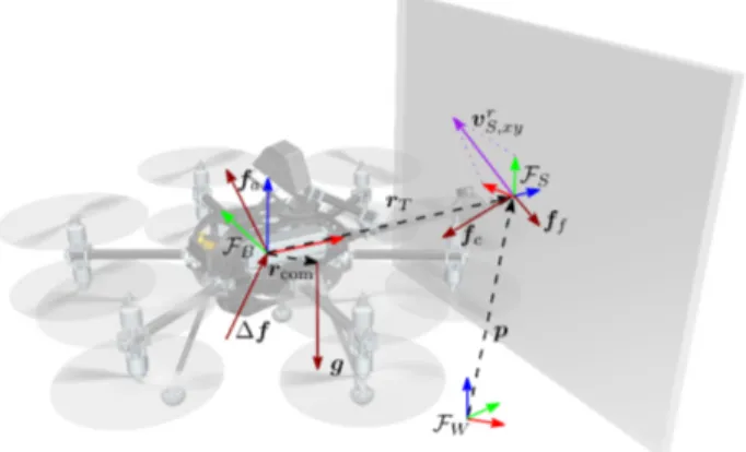
Fig. 1. Visual representation of the aerial manipulation system during a push-and-slide task, and its main variables.
the transition between static and dynamic contact becomes nontrivial. Larger static friction forces, if not properly ad- dressed, can cause saturation of the inputs, overshoots, and unexpected slips leading to possible crashes.
Passivity-based techniques have been implemented for fully actuated AMs, such as the energy tank approach, which aim to handle the problem of unwanted slippage or loss of contact. This is achieved by virtually dissipating an energy tank in the controller, and restricting the system output accordingly [7]. However, forces during push-and-slide tasks remain small, and there is no use of direct force sensing, nor anticipation of the future trajectory.
The knowledge of interaction forces at the end-effector (EE) can provide key insight into the consideration of friction-based contact constraints. The estimation of EE forces for AMs, however, is typically degraded by unmodeled aerodynamic effects and delays due to system integration.
With recent improvements of force-sensing technology, these concerns are addressed by directly measuring interaction forces with a Force-Torque (FT) sensor at the EE [8], [9].
Up to this point, existing control techniques for aerial interaction have been used for slow-moving, and predomi- nantly low-friction sliding interaction tasks. Model predictive control (MPC), with its ability to account for constraints and to optimize over the future trajectory with a receding horizon, offers a solution to this problem. MPC has been previously implemented with underactuated-base AMs with fixed [10]
and actuated [9] EE. However, due to underactuation of the platform, tasks remain slow, with low interaction forces dur- ing push-and-slide. Some MPC-based approaches have also been developed for fully-actuated MAVs [11], [12], but only in free-flight. In the domain of mobile robot manipulators,
direct interaction force control has been implemented with MPC, achieving large forces applied to the environment [13].
Thanks to the fixed nature of the base, high friction forces could be treated as disturbances without causing instability.
The challenge remains in how to formulate the aerial inter- action problem with a model-based controller in the presence of unknown environmental parameters, appropriately inte- grating information from direct force sensing. The method proposed in this paper aims to extend aerial interaction to high friction interaction up to high velocities. In particular, we present the following contributions:
• A novel nonlinear model predictive controller (NMPC) for hybrid 6-DoF pose and force tracking for a fully- actuated AM, incorporating direct force feedback for interaction.
• A practical implementation of contact constraint con- ditions for high friction aerial interaction, with au- tonomous transitions between 3 different control modes.
• Experimental validation of the controller and compar- ison against an impedance controller with a PI force feedback.
II. SYSTEM MODELING
In the course of this work we will refer to three ref- erence frames as depicted in Fig. 1: the inertial world frame FW ={OW,xW,yW,zW}, the body frame FB = {OB,xB,yB,zB} which is fixed to the geometric center of the AM, and the surface frameFS ={OS,xS,yS,zS}, which is fixed to the surface (assumed flat in the work-space) and arbitrarily placed.O?represents the center of the generic frameF?, while (x?,y?,z?) represent its unit axes. Notice that FS is defined s.t.zS is orthogonal to and oriented into the surface. Additionally, FW is defined s.t.zW is aligned with the gravity vectorg∈R3.
The position of the EE and of the body center of mass (CoM) w.r.t. FB are represented by the vectors rT ∈ R3 and rcom ∈ R3, respectively. We assume that the AM and its EE are parts of a single rigid body, i.e.,rT andrcom are constant.
We introduce the flight control factor λ ∈ {0,1}, where the system can be i) in free flight andλ= 0, or ii) in contact with a surface andλ= 1. In free flight the system’s motion is unconstrained, while in contact, the EE can move only on a plane defined by{xS,yS}. To define interaction constraints according to the flight mode expressed by λ, we use the following selection matrix that will later be employed in the derivation of the dynamics:
Sλ=RSdiag(1,1,1−λ)R>S, (1) whereRS ∈SO(3)represents the attitude ofFS w.r.t.FW. The system mass and inertia w.r.t. FB are denoted by m ∈ R>0 and J ∈ R3×3>0 . Forces and torques acting on the system include i) those produced by the actuators of the aerial platform, fa ∈ R3 and τa ∈ R3, expressed in FB, ii) the contact force fc ∈ R3, expressed in FW, iii) the gravitational force mg, expressed in FW, iv) and general disturbance forces and torques, ∆f ∈ R3 and ∆τ ∈ R3, expressed inFW andFB, respectively.
Since we are interested in controlling the pose of the EE, we consider as configuration of the system the position and orientation of the EE w.r.t.FW described by the vector p∈R3 and the quaternion q∈H, respectively. Their time derivatives, i.e., the linear and angular velocity w.r.tFW, are given by the vectorsv∈R3 andω∈R3, expressed in FW
and FB, respectively. We can write the system dynamics using the Newton-Euler equations:
˙
p=Sλv (2a)
˙
v=Sλ(aB+RB( ˙ω×rT+ω×ω×rT)) (2b)
˙ q= 1
2q⊗ 0
ω
(2c)
˙
ω=J−1(τa−ω×(J ω) +rcom×(R>Bmg)
| {z }
τcom
+rT ×(λR>Bfc)
| {z }
τc
+∆τ) (2d)
aB=m−1(RBfa+λfc+ ∆f) +g. (2e) The actuation and disturbance forces fa and ∆f are assumed to act directly on the geometric center, which results in the body accelerationaB.
The matrixSλimplements the constraints imposed by the contact with the surface. In particular, it truncates the linear dynamics in (2a) and (2b) along zS (the surface normal direction) if λ = 1. Additionally, the contact force fc is only considered in (2d) and (2e) ifλ= 1.
III. CONTROL DESIGN A. Overview
We aim to integrate and address the interaction effects discussed in Section I by designing a controller with the following properties:
(a) Hybrid tracking of the EE pose and contact force according to a pose/force reference trajectory. The force control should use a FT sensor for direct force feedback compensating uncertainties and external disturbances.
(b) Autonomous transitioning between contact-less and contact-based flight control, accounting for interaction constraints affecting the system dynamics.
(c) Autonomous transitioning between static and dynamic friction control.
(d) Incorporation of bounds on the dynamics and reference to account for infeasible trajectories and inputs.
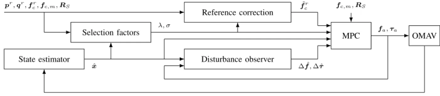
In order to achieve these properties, we use an MPC ap- proach with a variable model and variable weights. Both the model and the weights are dynamically updated according to the current control mode. Figure 2 gives an overview of the entire control structure.
B. Control modes
From practical and general friction model considerations, we separate a push-and-slide interaction task into three different control modes: 1) free flight, 2) stiction (i.e. static force control), and 3) sliding (i.e. dynamic force control).
As we use a model-based controller, we would like to integrate the knowledge about the current control mode.
Preprint version, final version at http://ieeexplore.ieee.org/ 2 IEEE International Conference on Robotics and Automation 2021
Selection factors
Disturbance observer Reference correction
MPC OMAV
State estimator
fa,τa
pr,qr,fcr,fc,m,RS
λ, σ
ˆ x
f˜cr fc,m,RS
∆ ˆf,∆ ˆτ
Fig. 2. Control diagram.
Control mode λ σ Reference tracking
Free flight 0 N/A 3-DoF Position, Attitude Static force control 1 0 2-DoF Position, Attitude, Force Dynamic force control 1 1 2-DoF Position, Attitude, Force TABLE I. Control modes as a result of the selection factorsλandσ.
Therefore, we will use both state and reference trajectory information to change the model dynamics of the MPC as well as the controller tuning.
With this aim, we introduce twoselection factors, namely λ∈ [0,1] andσ ∈[0,1], to distinguish these three modes.
Theflight control factorλ(already introduced in Section II) represents the transition between contact-less and contact- based flights. Additionally, we use theforce control factorσ to represent the transition between stiction and sliding control modes. In detail, the relation between control modes and selection factors is the following:
• Free flight (FF),λ= 0: the MAV moves in space, while there is no interaction with the surface.
• Static force control (SFC),λ= 1, σ= 0: the MAV is in contact with the surface and the EE position is constant.
Notice that the orientation of the EE can change. The interaction force stays in the friction cone of the EE.
• Dynamic force control (DFC), λ= 1, σ= 1: the MAV is in contact with the surface and the EE linear velocity is non-zero. The orientation of the EE can change. In this case, dynamic friction is acting on the EE.
Table I gives an overview of the available control modes and which states are tracked accordingly.
The current control mode, i.e. the combination ofλandσ, is determined by fusing state and reference trajectory infor- mation. It is therefore not a direct result of the optimization, but rather a condition that influences the optimization.
In order to create smooth transitions between the modes, we will use a cosine step function that interpolates between 0 and 1 in a given range[x, x]⊂R:
l(x, x, x) =
0, if x≤x
1 2
1−cos
x−x x−xπ
if x < x≤x
1, otherwise
. (3)
For the remainder of this text, we use the superscript ·r to denote reference variables.
1) Computation ofλ: The calculation of the flight control factorλis done in a similar fashion as in [14] and depends on the current contact force measurement, fc,m ∈R3, and
the position error projected onto the contact force reference, ep∈R, computed as:
ep =
((p−pr)·kffcrr
ck, if kfcrk>0
(p−pr)·zS, otherwise . (4) We design λ such that the current mode is detected as interaction, if the magnitude of the measured contact force, kfc,mk, is above a threshold fc,max∈R and if simultane- ously the projected position error ep is below a threshold ep,min ∈ R. In any other case the mode defaults to being in free flight. While in interaction, we intend to not track the EE position in the surface normal direction. Therefore, we use ep as trigger to detach from the surface once the reference demands it.
In order to allow smooth transitions, we additionally use a minimum force measurement and a maximum position error threshold, fc,min ∈ R and ep,max ∈ R, respectively. We therefore construct two auxiliary variables λf ∈ [0,1] and λe∈[0,1]which are later merged to compute λ.
λf =l(kfc,mk, fc,min, fc,max)
λe= 1−l(ep, ep,min, ep,max). (5) Based on the definition ofλfandλe, the AM is in interaction if both variables are 1. To avoid high noise in the evaluation of this AND condition on continuous variables, we employ amin function and apply a low-pass filter with gain aλ ∈ [0,1]. This results in the following relation for the selection factor at time stepk∈N≥0:
λk =λk−1+aλ(min(λf, λe)−λk−1). (6) 2) Computation ofσ: The force control factorσdifferen- tiates between static and dynamic force control, i.e. between stiction and sliding friction. We use this distinction to enable different tuning of the controller for different control modes.
We combine a simple assumption about stiction physics and the current velocity reference to determine if the con- troller should expect static or dynamic friction:
• If the friction force norm is below a certain threshold ff,min∈R,or
• if the norm of the reference velocity projected onto the surface, is above a thresholdvS,maxr ∈R,
then the control mode is DFC, otherwise it is SFC.
By following this approach, we assume that a friction force below a threshold ff,min indicates dynamic friction (i.e. sliding), while a friction force estimate above a higher
thresholdff,max∈Rindicates static friction (i.e. no lateral movement possible).
Instead of estimating the friction force, we form a friction force envelope ff ∈R to keep track of the recent maximal friction force norm. This is implemented by applying a low- pass filter with different rise and fall times to the projection of the measured interaction force onto the surface:
ff,k =ff,k−1+af,k∆ff,k, with af,k =
(arise, if ∆ff,k>0
afall, otherwise , ariseafall
∆ff,k =kdiag(1,1,0)R>S,kfc,m,kk −ff,k−1. (7)
We use a high arise ∈ [0,1] to be responsive to increasing friction forces and a low afall ∈ [0,1] to avoid too fast transitions to DFC. That way,ff represents the friction force envelope, i.e. an estimate of the highest achieved friction force. Furthermore, we use the projected norm of the velocity reference which is computed as:
vrS,xy=kdiag(1,1,0)R>Svrk. (8) As before, for the computation ofσwe rely on two auxiliary variablesσf ∈[0,1]andσv∈[0,1]computed as follows
σf = 1−l(ff, ff,min, ff,max) σv =l vrS,xy, vS,minr , vS,maxr
. (9)
Since by its definition,σis 0 if bothσf and σv are 0, and 1 otherwise, we use amaxfunction and a low-pass filter with gainaσ∈[0,1]to compute the force control factor:
σk=σk−1+aσ(max(σf, σv)−σk−1). (10) C. Model Predictive Control
As a state vector, we use the force and torque generated by the actuators,fa andτa, the EE positionp and velocity v, as well as the body orientation q and angular velocity ω. The input vector is composed of the actuator force and torque time derivatives,f˙a andτ˙a:
x=
fa> τa> p> v> q> ω>>
∈ X ⊂R19 u=h
f˙a
> τ˙a>i>
∈ U ⊂R6.
(11) The system dynamics employed in the MPC, defined by xk+1 = fk(xk,uk), include discretized equations (2a) to (2e) and the relation [ ˙fa> τ˙a>]> = I6u, where Im ∈ Rm×m is the identity matrix of dimension m ∈N>0. The receding horizon MPC problem is given by:
u0,...uminN−1
N−1
X
k=0
khx(xk,xrk)k2Qx+khu(uk,urk)k2Qu
+khx(xN,xrN)k2QN s.t. xk∈ X,uk ∈ U,
xk+1=fk(xk,uk), x0= ˆx(t),
λk=λ(t), RS ,k=RS(t), fc,k=fc,m(t),
∆fk= ∆ ˆf(t), ∆τk= ∆ ˆτ(t).
(12)
The disturbance estimates ∆ ˆf ∈ R3 and ∆ ˆτ ∈ R3 are obtained by a disturbance observer. The cost function is composed of the cost vectors weighted norms with matrices Qx ∈ R15×15≥0 , Qu ∈ R6×6>0 , and QN ∈ R15×15≥0 . The cost matricesQxandQu are constant throughout the prediction horizon. We formulate the cost vectors in a way to meet two objectives simultaneously:
• Minimize the EE pose error;
• Minimize the force tracking error, if a reference force is available and if contact with a surface is established.
The first objective is implemented by using cost terms on the predicted pose and twist error at each time step of the horizon. The attitude error is approximated inR3 according to [15]. The second objective is achieved by penalizing the difference between the predicted contact force and the force reference at the tip of the EE. The cost vectors are therefore defined as:
hx(xk,xrk) =
efck
pk−prk vk−vrk Im(qk⊗(qrk)−1)
ωk−ωrk
∈R15
hu(uk,urk) = f˙a,k
˙ τa,k
∈R6.
(13)
To compute the contact force errorefc, we define a corrected force referencef˜cr∈R3, whose computation will be detailed in the next paragraph. The contact force error is then defined as the difference between the contact force and the contact force reference:
efc=mSλarB−RBfa−mg−∆f
| {z }
fc
−f˜cr. (14) a) Force reference correction: We apply a contact force reference correction with the following two objectives:
Firstly, in SFC, i.e. when the EE is not moving, we want the measured contact force fc,m to converge to the reference forcefcr. In this case, we correct the reference force by the current force tracking error. We use a proportional-integral correction to avoid steady-state tracking offsets. Secondly, in DFC, we do not apply this correction, as EE needs to overcome static friction forces to track a position reference.
We differentiate between these two cases by introducing the control-mode dependent matrixSσ:
Sσ=λfRSdiag(1−σ,1−σ, λ)R>S, Sσ∈R3×3 f˜cr=fcr+Sσ
Kp(fcr−fc,m) +Ki
Z
(fcr−fc,m)dt
. (15) b) Constraints on inputs and states: The sets of states X and inputsU are constructed to limit actuator wrench and its derivative similarly as in [11]. In this way, the MPC is aware of the system’s physical constraints.
c) Dynamic updating of weight matrices: We de- fine three independent weight matrices QF F, QSF C, and QDF C ∈ R15×15, and fuse them according to the current control mode. The terminal stage weight QN is computed as the scaled version of the stage weight Qx by the static
Preprint version, final version at http://ieeexplore.ieee.org/ 4 IEEE International Conference on Robotics and Automation 2021
gainaN ∈R>0. The block-diagonal matrix RS transforms the axis-specific weight tuning from the surface frame into the world frame.
Qx= (1−λ)QF F
+λRS((1−σ)QSF C+σQDF C)R>S, (16a)
QN =aN ·Qx, with (16b)
RS =blockdiag(RS,RS,RS,I3,I3). (16c) D. Disturbance observer
We employ the same EKF-based disturbance observer as in [11]. Similarly to equations (2a) to (2e), it models the AM as a rigid body with disturbance forces and torques applied on FB. For simplicity, the model does not include interaction forces and no CoM offset. Therefore, its dy- namics are driven by the commanded wrench, fa and τa, corrected by contact force and CoM torque offsets. We use the measured body pose and twist as measurement vector zEKF =
p>B,m vB,m> qm> ωm>>
. The EKF state and input vector are then defined as
xˆ= ˆ
p>B vˆB> qˆ> ωˆ> ∆ ˆf> ∆ ˆτ>>
, (17a) uEKF =
fa+R>Bλfc,m
τa+rcom×(R>Bmg) +rT ×(R>Bλfc,m)
.
(17b) E. Actuator allocation
The final rotor speed and tilt angle commands are com- puted according to the allocation method presented in [16].
IV. EXPERIMENTS A. Experimental setup
We use a custom built AM similar to the one in [11].
Its design can be seen in Fig. 1. The platform consists of a body with 6 arms that each have 2 counter rotating propellers mounted. Each arm can individually be rotated by servos to allow for full 6-DOF wrench generation. A rigid carbon fiber tube is attached horizontally to the body center. At its end, a Rokubi FT sensor1 is placed in between the tube and an EE. The raw force measurements are filtered with a low-pass filter and then applied directly in the MPC formulation and in the EKF input (see (17b)). The body center comprises an Intel NUC and a Pixhawk flight controller. State estimation is performed by an EKF that fuses motion capture pose measurements from a VICON system and onboard inertial measurement unit (IMU) measurements. The AM is powered through a ground-based power supply2 whose lightweight cable can be extended to80 m, making it feasible for real- world applications. The total mass of the system is 5.2 kg.
We use a customary whiteboard as a contact surface, and a rubber ball with a diameter of approx. 2 cm as EE. Due to its suspension by cables, the whiteboard is not entirely rigid. Slight movements are regarded as disturbances in the dynamic modeling. The rubber ball has shown to generate
1https://www.botasys.com/rokubi
2https://elistair.com/safe-t-tethered-drone-station/
Relative weights efxy efz epxy epz eq
FF 0 0 1 1 1
SFC 1 1 0.1 0 1
DFC 0 1 0.25 0 1
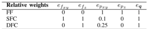
TABLE II. Relative tuning weights for different control modes.
high stiction and friction forces, making sliding tasks more difficult to control than low-friction EEs.
The MPC was implemented using the ACADO framework [17] in Robot Operating System (ROS). The controller computes control inputs at 100 Hz with an average MPC solving time of 5 ms. The MPC step size was chosen as 50 mswithN= 20steps, yielding a horizon length of1 s.
B. Experiments
Experiments are designed to evaluate the following char- acteristics of the controller:
• Position tracking of the EE on the surface,
• interaction force tracking,
• autonomous transitioning between the control modes and its effect on the tracking performance.
We use the following trajectory to evaluate these character- istics: Starting in front of a surface, the reference trajec- tory brings the EE in contact and commands a horizontal translation of0.8 mwith a velocity of up to0.6 m s−1while applying a constant force of3 N.
We compare the performance of our proposed MPC against an impedance controller that employs a PI force- feedback controller on the force measurements at the EE as used in [14].
C. Controller and threshold tuning
The weight matrices were manually tuned for each con- trol mode, balancing aggressive tracking that could lead to slippage of the tool and too soft tracking that could lead to stiction or to too large errors in attitude, resulting in the AM touching the surface.
We use different weight tunings for the three control modes as shown in Table II. Note that we apply different weights on different axes inFS, such that lateral and normal errors are penalized differently.
The thresholds for the control mode transitions are tuned as follows: To reliably detect contact with a surface, we set fc,min and fc,max to be well over the force sensor noise, and with enough difference to allow a continuous transition. In order to achieve continuous force control during the movement on the surface, we set ep,min and ep,max
large enough to allow small position errors due to possible irregularities in the surface shape.
The reference velocity thresholdsvS,minr andvrS,max are set to small values, as we expect sliding friction for any change in the reference position. The friction envelope thresholdsff,min andff,max are set based on experiments, such that they are larger than the friction force that we measured during sliding experiments. They are therefore dependent on the materials of the EE and the surface, as well as on the desired contact force.
The friction force is filtered according to (7) with arise = 0.05 and afall = 0.0005. Throughout all presented experi- ments, we used the tuning values as shown in Table III.
Threshold fc[N] ep[m] ff [N] vSr [m s−1]
·min 1.4 0.1 2.0 0.005
·max 1.6 0.15 4.0 0.01
TABLE III. Threshold tuning for mode transitions.
During preliminary experimental testing, we found that the use of the contact force measurement in the angular dynamics equation Eq. (2d) led to instabilities. We therefore removed the explicit computation of the contact torque τc from the system dynamics and the disturbance observer input Eq. (17b). As a consequence, its influence is captured by the disturbance estimate∆ ˆτ only. We assume that biases in the FT measurements, multiplied with the distance of the EE from the body center, lead to quickly varying torque compensation terms that destabilize the system.
D. Results
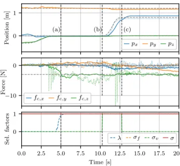
Figure 3 shows the position and force tracking during the sliding trajectory with a reference normal force of 3 N for both MPC and impedance controller. Additionally, the bottom plot shows the selection factors that trigger the transitions between control modes.
While the impedance controller shows good accuracy in position tracking, the sudden impact onto the surface and high friction forces during the translation lead to multiple detachments (at12 s) and unsteady contact force tracking.
The position tracking of the MPC shows that the EE overshoots the reference position after the translation, but then remains stable at the reached destination. We see the delay in the estimated disturbance torque as the main reason for the inaccurate position tracking. Nevertheless, the MPC is able to generate a smooth transition between free flight and contact, without creating force spikes. The flight control factor λ correctly tracks the transitions between FF and interaction control. Once the EE is in contact with the surface, the transition of λ from 0 to 1 enables the force tracking and disables the position tracking along the surface normal. Since the lateral friction force does not grow large enough to reach ff,min, the controller remains in DFC.
In Fig. 4, we repeated the sliding experiment with a higher force reference of 5 N. This resulted in a higher friction force, which triggered the transition from DFC to SFC after finishing the second translation. Under the influence of these high friction forces, DFC can lead to instabilities as a result of too aggressive lateral position tracking. On the other hand, SFC prioritizes force tracking in all directions and puts less emphasis on lateral position tracking, therefore stabilizing the AM after finishing the trajectory.
V. CONCLUSION
We presented an NMPC framework that considers the dynamics of an AM in free flight and two different force interaction modes to optimize the control inputs. Different control modes are used to change the tuning of the MPC
0 1
Position[m]
(a) (b) (c)
px py pz
−10 0
Force[N]
fc,x fc,y fc,z
0.0 2.5 5.0 7.5 10.0 12.5 15.0 17.5 20.0 Time [s]
0 1
Sel.factors
λ σf σv σ
Fig. 3. Position and force tracking of MPC (continuous) and Impedance controller (dotted line), inFS, withkfcrk= 3 N. Dashed lines represent the reference position and force. Vertical dashed lines indicate the different interaction modes: before (a): free flight, (a)-(b): static interaction, (b)-(c):
dynamic interaction, after (c): static interaction. The bottom plot shows the selection factorsλandσ.
0 10 20 30 40
Time [s]
0.0 0.5 1.0
Selectionfactors λ
σf
σv
σ
Fig. 4. Selection factors for sliding force tracking withkfcrk= 5 N.
weights as well as the constraints on the system dynam- ics. The controller autonomously transitions between these different modes based on the reference trajectory and state estimates. The use of a FT sensor allows for direct force con- trol at the EE. Push-and-slide experiments with high friction coefficients have validated the transitioning between control modes as well as accurate normal force tracking, showing improvements with respect to the impedance controller. Non- linear friction behaviours due to stiction remain a difficult challenge that needs to be tackled in the future. This would enable sliding interaction tasks with higher required normal forces. While experiments have been performed with high accuracy pose tracking provided by VICON, in real-world applications, we will investigate the use of onboard Visual- Inertial Odometry in combination with GPS to estimate the AM’s relative pose to its environment.
REFERENCES
[1] F. Ruggiero, V. Lippiello, and A. Ollero, “Aerial Manipulation: A Literature Review,” IEEE Robotics and Automation Letters, vol. 3, no. 3, pp. 1957–1964, 2018.
Preprint version, final version at http://ieeexplore.ieee.org/ 6 IEEE International Conference on Robotics and Automation 2021
[2] R. Rashad, J. Goerres, R. G. Aarts, J. B. Engelen, and S. Stramigi- oli, “Fully Actuated Multirotor UAVs: A Literature Review,” IEEE Robotics & Automation Magazine, 2020.
[3] M. Ryll, G. Muscio, F. Pierri, E. Cataldi, G. Antonelli, F. Caccavale, and A. Franchi, “6D Physical Interaction with a Fully Actuated Aerial Robot,” in2017 International Conference on Robotics and Automation (ICRA), Singapore, May 2017, pp. 5190–5195.
[4] S. Park, J. Lee, J. Ahn, M. Kim, J. Her, G.-H. Yang, and D. Lee,
“Odar: Aerial manipulation platform enabling omnidirectional wrench generation,”IEEE/ASME Transactions on mechatronics, vol. 23, no. 4, pp. 1907–1918, 2018.
[5] K. Bodie, M. Brunner, M. Pantic, S. Walser, P. Pfndler, U. Angst, R. Siegwart, and J. Nieto, “An Omnidirectional Aerial Manipulation Platform for Contact-Based Inspection,” Robotics: Science and Sys- tems XV, 2019.
[6] M. Tognon, H. A. T. Ch´avez, E. Gasparin, Q. Sabl´e, D. Bicego, A. Mallet, M. Lany, G. Santi, B. Revaz, J. Cort´es et al., “A truly- redundant aerial manipulator system with application to push-and-slide inspection in industrial plants,”IEEE Robotics and Automation Letters, vol. 4, no. 2, pp. 1846–1851, 2019.
[7] R. Rashad, J. B. Engelen, and S. Stramigioli, “Energy tank-based wrench/impedance control of a fully-actuated hexarotor: A geometric port-hamiltonian approach,” in 2019 International Conference on Robotics and Automation (ICRA). IEEE, 2019, pp. 6418–6424.
[8] G. Nava, Q. Sabl, M. Tognon, D. Pucci, and A. Franchi, “Direct Force Feedback Control and Online Multi-Task Optimization for Aerial Manipulators,”IEEE Robotics and Automation Letters, vol. 5, no. 2, pp. 331–338, 2020.
[9] D. Tzoumanikas, F. Graule, Q. Yan, D. Shah, M. Popovic, and S. Leutenegger, “Aerial Manipulation Using Hybrid Force and Position NMPC Applied to Aerial Writing,” 2020.
[10] K. Alexis, G. Darivianakis, M. Burri, and R. Siegwart, “Aerial robotic contact-based inspection: planning and control,”Autonomous Robots, vol. 40, no. 4, pp. 631–655, 2016.
[11] M. Brunner, K. Bodie, M. Kamel, M. Pantic, W. Zhang, J. Nieto, and R. Siegwart, “Trajectory Tracking Nonlinear Model Predictive Control for an Overactuated MAV,” in2020 IEEE International Conference on Robotics and Automation (ICRA), 2020, pp. 5342–5348.
[12] D. Bicego, J. Mazzetto, R. Carli, M. Farina, and A. Franchi, “Non- linear Model Predictive Control with Enhanced Actuator Model for Multi-Rotor Aerial Vehicles with Generic Designs,”Journal of Intel- ligent & Robotic Systems, pp. 1–35, 2020.
[13] J. Pankert and M. Hutter, “Perceptive Model Predictive Control for Continuous Mobile Manipulation,” IEEE Robotics and Automation Letters, vol. 5, no. 4, pp. 6177–6184, 2020.
[14] K. Bodie, M. Brunner, M. Pantic, S. Walser, P. Pfndler, U. Angst, R. Siegwart, and J. Nieto, “Active Interaction Force Control for Omnidirectional Aerial Contact-Based Inspection,” 2020.
[15] J. Sola, “Quaternion kinematics for the error-state kalman filter,”arXiv preprint arXiv:1711.02508, 2017.
[16] K. Bodie, Z. Taylor, M. Kamel, and R. Siegwart, “Towards Efficient Full Pose Omnidirectionality with Overactuated MAVs,”Proceedings of the 2018 International Symposium on Experimental Robotics, p.
8595, 2020.
[17] B. Houska, H. Ferreau, and M. Diehl, “An Auto-Generated Real-Time Iteration Algorithm for Nonlinear MPC in the Microsecond Range,”
Automatica, vol. 47, no. 10, pp. 2279–2285, 2011.
Preprint version, final version at http://ieeexplore.ieee.org/ 7 IEEE International Conference on Robotics and Automation 2021