Isolation and Subjective Welfare:

P ^olicy R ^eseaRch W ^oRking P ^aPeR 4535

Isolation and Subjective Welfare:

Evidence from South Asia

Marcel Fafchamps Forhad Shilpi

The World Bank

Development Research Group

Sustainable Rural and Urban Development Team February 2008

WPS4535

Public Disclosure AuthorizedPublic Disclosure AuthorizedPublic Disclosure AuthorizedPublic Disclosure Authorized

Abstract

The Policy Research Working Paper Series disseminates the findings of work in progress to encourage the exchange of ideas about development issues. An objective of the series is to get the findings out quickly, even if the presentations are less than fully polished. The papers carry the names of the authors and should be cited accordingly. The findings, interpretations, and conclusions expressed in this paper are entirely those of the authors. They do not necessarily represent the views of the International Bank for Reconstruction and Development/World Bank and its affiliated organizations, or those of the Executive Directors of the World Bank or the governments they represent.

Policy ReseaRch WoRking PaPeR 4535

Using detailed geographical and household survey data from Nepal, this article investigates the relationship between isolation and subjective welfare. This is achieved by examining how distance to markets and proximity to large urban centers are associated with responses to questions about income and consumption adequacy. Results show that isolation is associated with a significant reduction in subjective assessments of income and consumption adequacy, even after controlling

This paper—a product of the Sustainable Rural and Urban Development Team, Development Research Group—is part of a larger effort in the department to understand the impact isolation on subjective measure of economic welfare. Policy Research Working Papers are also posted on the Web at http://econ.worldbank.org. The author may be contacted at fshilpi@worldbank.org.

for consumption expenditures and other factors. The reduction in subjective welfare associated with isolation is much larger for households that are already relatively close to markets. These findings suggest that welfare assessments based on monetary income and consumption may seriously underestimate the subjective welfare cost of isolation, and hence will tend to bias downward the assessment of benefits to isolation-reducing investments such as roads and communication infrastructure.

Isolation and Subjective Welfare: Evidence from South Asia

Marcel Fafchamps

Oxford University

Forhad Shilpi

The World Bank

JEL codes: D60, I31, R20

Keywords: geographical isolation; consumption adequacy; subjective well-being

*

We benefitted from comments from Ravi Kanbur, Mukesh Eswaran, John Hoddinott, John Pender, Martin Ravallion, and participants to a seminar at Cornell and IFPRI. We also received excellent comments on an earlier version of this paper from participants to the Cornell/LSE/MIT Conference on Behavioral Economics, Public Economics and Development Economics; participants to the Global Poverty Research Group workshop held in June 2004;

and from participants to seminars at LSE, CERDI, the University of British Columbia, Bath University, and the World Bank. We would like to thank Migiwa Tanaka for excellent research assistance. The support of the World Bank and of the Economic and Social Research Council (UK) is gratefully acknowledged. The work was part of the programme of the ESRC Global Poverty Research Group.

†

Department of Economics, University of Oxford, Manor Road, Oxford OX1 3UQ. Email:

marcel.fafchamps@economics.ox.ac.uk.

‡

DECRG, The World Bank, 1818 H Street N.W., Washington DC 20488 USA..

1. Introduction

While much has been written on the relationship between geographical location and objec- tive measures of consumption and welfare (e.g. Elbers, Lanjouw & Lanjouw 2003, Jalan &

Ravallion 2002, Ravallion & Jalan 1996, Ravallion & Jalan 1999, Ravallion & Wodon 1999), little is known on how isolation affects subjective welfare. The traditional literature on labor migration has often assumed that rural dwellers prefer living in the countryside and would have to be compensated for migrating to town. This assumption, for instance, underlies original contributions by Lewis (1954) and Harris & Todaro (1970). More recently, Murphy, Shleifer &

Vishny (1989) make a similar assumption regarding wage work. Little hard evidence however exists on the utility cost or benefit of rural living.

This paper revisits the question of the relationship between isolation and subjective welfare and estimates the welfare cost of geographic isolation. To this effect, we use answers to subjective questions about consumption and income adequacy to test whether utility is equalized across space and, if it is not, whether utility is higher or lower in isolated areas. This approach enables us to investigate in a direct and straightforward manner the question of the relationship between isolation and utility without requiring any assumption about spatial mobility.

The starting point of our empirical specification is a standard utility maximization model in

which isolation is related to utility through its effect on incomes and prices, on the availability of

goods and services, and on public goods and externalities. For our empirical investigation, we use

a large-scale living standard measurement survey, the Nepal Living Standard Survey (NLSS) of

1995/96. Nepal is the perfect country to study isolation because so much of the country remains

inaccessible by road. The NLSS includes a number of questions on subjective consumption and

income adequacy. The head of each surveyed household was asked to rank the household’s total

income as ‘not adequate’, ‘adequate’ or ‘more than adequate’. Similar questions were asked

about

We investigate whether responses to these questions vary systematically with distance to markets and cities.

Our econometric investigation leads to a robust

subjective welfare. This result obtains after we control for consumption expenditures, suggesting that the relationship between isolation and welfare is not only due to lower monetary consump- tion. Controlling for household mobility and adding various controls leaves results unchanged.

We quantify the difference in subjective welfare associated with isolation and

particularly for housing, schooling and health care. Surprisingly, the reduction in subjective wel- fare associated with isolation is largest for households already close to markets. These results should be interpreted as indicative of a strong empirical relationship between geographical isola- tion and subjective welfare. Better data is needed to ascertain the causal effect of geographical isolation on welfare.

The paper is organized as follows. The conceptual framework is discussed in Section 2.

Section 3 describes the data and its main characteristics. Econometric estimation results are presented in Section 4 while in Section 5 we quantify the reduction in subjective welfare asso- ciated with geographical isolation. Section 6 discusses the results and Section 7 concludes the paper.

2. Conceptual framework

For the sake of this paper, let us define isolation as distance from urban centers: a household located at a large distance

from the nearest urban center is deemed to be more isolated than a household located closer. We are interested in the relationship between welfare and local

1Other surveys have also asked what is typically referred to as the subjective well-being question, namely, ’Do you feel generally happy with life?’. Unfortunately, this question was not asked in the NLSS.

characteristics. To capture this idea, let individuals derive utility

from total consumption expenditures

and from public amenities

V_jk=V(X_jk, A_k)

where

denotes the individual and

the location. To keep the presentation simple, other factors such as prices, product variety, etc, are ignored for now. We introduce them later. We ignore savings, so that income equals consumption.

Individuals prefer the location

where their utility

is highest. Whether they can relocate or not depends on the functioning of the labor market. We

locate freely and costlessly. We then examine the case where workers are immobile or move at a cost.

2.1. The cost of isolation

Assume for a moment that

is the same across locations. If individuals can move at no cost, arbitrage implies that utility — and hence income — are equalized across locations. To generate different levels of income and utility across locations, let us follow Roy (1951), as modified by Dahl (2002), and assume that workers differ in ability

so that some individuals have higher marginal productivity. In a competitive labor market with free movement of labor, workers are paid their marginal product. We thus have

with

Now assume that, for technological reasons, jobs that require a high ability are located in or near cities, i.e., that

With these assumptions, average welfare is higher

2This is not an unreasonable assumption. Fafchamps & Shilpi (2005), for instance, have shown that there are largerfirms and more job specialization in and around cities. We also know from the work of Jacoby (2000) that, in Nepal, land located far from markets has a lower value and yields a lower income. This is undoubtedly due to lower average prices for agricultural output and less emphasis on commercial farming, an issue that is revisited by Fafchamps & Shilpi (2003). All these factors probably generates higher returns to education and to entrepreneurial ability in urban centers.

in cities, i.e.,

urban centers where wages are higher. If we assume that ability has no direct effect on utility, welfare differences across locations and individuals are entirely driven by differences in income.

Once we condition on income, we should observe no systematic relationship between utility and urban proximity, i.e.,

Now assume that market towns and other urban centers have better amenities — higher

This could be because it is less costly to provide public services to a concentrated population.

Since workers locate freely, arbitrage implies that:

V(Xk(εj), Ak) =V(Xm(εj), Am)

where

and

denote two different locations. It follows that

if

: for a given ability

, workers in high

areas receive a lower wage than workers in low

areas (e.g.

Rosen 1979, Roback 1982).

By assumption

is a decreasing function of distance from cities.

It follows that

This generates testable predictions. If we compare two workers earning the same income but living in locations with different levels of amenities

location has higher ability, and thus higher utility. There is a negative relationship between utility and amenities — proxied by distance — after we control for income. It is possible to measure the implicit value of amenities by comparing wages of similar ability workers across locations with different levels of amenities. This is the approach adopted, for instance, by Rosen (1979) and Roback (1982).

Alternatively, suppose we do not observe ability but we observe a strictly increasing monotonic

3Of course, since ability is higher in urban areas, the average income across workers of different abilities is higher in urban areas and∂E[Xk(εj)]/∂dk<0where the expectation is taken over all abilitiesε.

transformation

implies that

. Further suppose that we do not observe

but

. We can estimate the implicit utility cost of isolation by regressing

on

and

:

W_jk =α₀+α₁logX_jk−α₂logd_k+u_jk

(2.1)

Differences in utility across location reflect differences in ability, but by comparing individuals with the same utility and different consumption

we identify the effect of distance

on utility.

Indeed, controlling for

, utility

falls with distance from urban centers as amenities get worse. This simple observation constitutes the basis of our testing strategy.

To compute the equivalent variation of isolation, let

denote the percentage of income that makes individual

indifferent between distance

and distance

. We have:

α0+α1logXjk−α2logdk+uj = α0+α1log(Xjk−CkmXjk)−α2logdm+uj

logX_jk(1−C_km) = α2

α₁(logd_k−logdm) logX_jk C_km = 1−e

α2

α1(logdk−logdm)

(2.2)

In case workers are immobile, the method proposed by Rosen (1979) and Roback (1982) breaks down. Since utility is not equalized across locations, it cannot be assumed that better amenities are compensated by lower wages, and wage differences across locations for workers of the same ability cannot be interpreted as the hedonistic price of better amenities.

The utility approach still works, however. It also works if workers can only move at a cost,

or if some individuals can move and others cannot — for instance because of credit constraints

or of discrimination in the labor market. This feature is particularly appealing given the kind

of data we have. Labor markets in Nepal are not as

(Dahl 2002), over 30% of US employees work in a state other than their birth state. In contrast, in Nepal, a country of 20 million people, more than 80% of household heads reside and work in their birth

mobile — only that, in each ability category and each location, some workers be mobile so that, at the margin, the arbitrage argument works. But with so many workers immobile, it is likely that arbitrage fails for at least some locations and some ability categories, therefore invalidating the Roback test. Furthermore, the overwhelming majority of Nepalese people are self-employed.

Their income depends on dimensions of individual ability that are difficult to measure — such as experience, familiarity with local conditions, and entrepreneurial spirit. It is therefore unlikely that we would be able to control for ability sufficiently well to measure the value of amenities using the Roback approach.

2.2. Multiple subjective satisfaction indicators

So far we have discussed the case of a single utility indicator. Now suppose that we have sub- jective satisfaction indicators for consumption subsets

such as food or clothing. To integrate these indicators into the analysis, we decompose consumption into

subsets and we assume that utility is (approximately) Cobb-Douglas with respect to these subsets. We start by ignoring amenities

subscripts for easier reading, we have:

V = [H h=1

ω_hlogc_h

4Dahl (2002) proposes a way of dealing with selection on unobserved ability. This solution requires not only a number of additional assumptions but also massive amounts of data to compute migration probabilities between each location. Unfortunately we do not have sufficient data to compute such transition matrices for Nepal.

where the

’s are consumption shares, with

ωh = 1. LetV^h

be the sub-utility obtained from the consumption of good

V^h = logc_h

If the consumer chooses consumption optimally, we have:

V = [H

h=1

ω_hlogω_hX ph

= a+ logX−logP

where

is a constant and

is a price index defined as

h

p^ω_h^h

. Similarly we can write:

V^h = logω_hX ph

= b+ logX−logph

where

is a constant.

To introduce geographical isolation, suppose that

where parameter

captures differences in amenities and in transport costs across consumption subsets. Taking logs we get:

V^h =b + logX−λ_hlogd

(2.3)

By comparing

across consumption subsets, we can infer which consumption subsets are most sensitive to isolation.

In practice, we do not observe

directly but a proxy

, namely the likelihood of answering

‘inadequate’, ‘adequate’ or ‘more than adequate’ to a consumption adequacy question for subset

h. Regression estimation yields:

W^h = g_h(V^h) =α^h₀+α^h₁logX−α^h₂logd

V^h = g_h⁻¹(α^h₀+α^h₁logX−α^h₂logd)

(2.4)

Totally differentiating (2.4) and (2.3) and setting them equal, we get:

∂V^h

∂logX = ∂g_h⁻¹

∂V^hα^h₁ = 1

∂V^h

∂logd = −∂g_h⁻¹

∂V^hα^h₂ =λ_h

from which it follows that:

λ_h ≈ α^h₂

α^h₁

(2.5)

where the approximation comes from the fact that we are averaging over observations. The equivalent variation

of isolation can be calculated for each consumption subset using

from equation (2.2).

So far we have assumed that consumers face no quantitative rationing. This may be a reason- able assumption for many goods but it is inadequate for public goods such as law enforcement or clean air. It is also problematic for goods that are publicly provided at a subsidized price,

5Product diversity can also be introduced to the model as follows. Assume that to each consumption subset hthere corresponds an aggregation function of the form:

ch= ] N_h

0

c(s)^ϕds _ϕ¹

wheresdenotes a continuum of goods andNhdetermines the range of goods available. If the prices of all goods are identical, we havech=chN

1 ϕ

h. Inserting into the utility function, we obtain an extra term:

V^h=b+ logX−logph+ 1 ϕlogNh

This shows that utility decreases with a fall in variety Nh, resulting for instance from isolation. To simplify notation, we omit varietyNhfrom the rest of the presentation.

such as health care. For these amenities, quantitative rationing arises if individuals are unable to purchase what they wish to consume at the subsidized price.

To illustrate this case, let us partition goods into rationed

and unrationed

Many amenities fall into the rationed category. Utility is written:

V = [U u=1

ω_ulogc_u+ [R r=1

ω_rlogc_r

(2.6)

where

is regarded as exogenously determined — it is not a choice parameter of the household.

Define

p_rc_r

. Utility maximization over the unrationed goods yields the familiar demand functions

u

and the indirect utility function can be written:

V =b+ logX_u−logP_u+ [R r=1

ω_rlogc_r

(2.7)

As we can see, utility now depends also on the consumed quantity of public goods and rationed public services. Suppose that

varies with isolation

on

and distance

also captures difference in

r=1ω_rlogc_r

, the value of which is included in the equivalent variation of isolation

.

When we look at specific consumption subsets, however, the utility derived from

drops out:

V^u = logcu

= b+ logXu−logpu

(2.8)

6By rationing we mean that the consumer is offhis demand curve. If limited supply of a good, say l, results in a high price in locationk, we do not regard this as rationing: since the consumer is on his demand curve, the formulas for the unrationed goods apply.

From this difference between (2.7) and (2.8), it follows that comparing

for total consump- tion with

for specific consumption subsets provides information about the isolation cost associated with public goods.

For rationed goods

we have:

V^r= logc_r

Suppose that

. It follows that

of the form:

W^r=gr(V^r) =α^r₀−α^r₂logd

This suggests a way of identifying rationed goods: for them, total expenditures

do not enter the regression.

Since expenditures do not enter the equation for

, we cannot estimate

using (2.5) because we do not have

. We may, however, obtain an order of magnitude for

if we are willing to make some strong assumptions regarding the way subjective adequacy questions were answered. Suppose we are willing to assume that

individuals answer adequacy questions about one subset in a way that is commensurate to the contribution of the subset to total utility. If this were the case,

would be the same for all unrationed goods and we could also use it to normalize the welfare cost of isolation for rationed goods:

λ_r ≈ α^r₂

α^u₁

(2.9)

If we have different unrationed goods

, one for each

7It is imporant to recognize that this comparison holds strictly only for Cobb-Douglas preferences. For more general preference functions, the consumption of amenities cr may affect satisfaction derived from unrationed goods because of complementarities between subsets. We revisit this issue below.

8It is conceivable that consumption is rationed for certain consumers but not others. we will be estimating a model that is a mixture of the rationed and unrationed case. Although we do not discuss this case explicitly here, it is intuitively clear that, as a result of attenuation bias, the coefficient of total expenditures will be smaller.

unrationed good

. If estimates of

for unrationed goods are relatively similar, we may hope that — should good

be unrationed — its

would fall within the same range. With these strong assumptions, we can ‘bracket’

and, by extension,

.

3. The data

The data we use come from the Nepalese Living Standard Measurement Survey (LSMS) of 1995/96. The survey drew a nationally representative sample of 3373 urban and rural households spread among 274 villages or ‘wards’. Between 16 and 20 households were interviewed in each ward. As with other LSMS surveys, data coverage of NLSS 1995/96 is quite comprehensive.

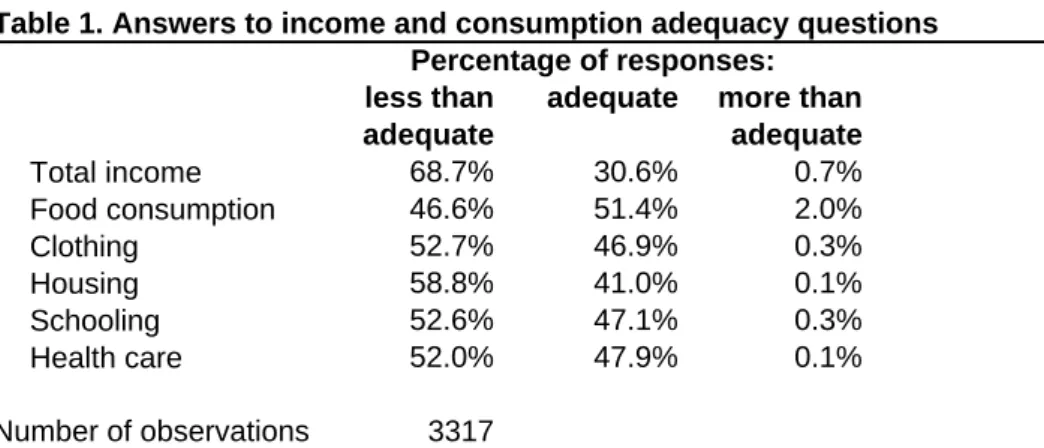
The survey includes a series of questions on the adequacy of consumption level enjoyed by the household. The household head was

family’s food consumption over the past one month], which of the following is true? It was less than adequate for your family’s needs [1], it was just adequate for your family’s needs [2], it was more than adequate for your family’ needs [3]." The household head was then asked

other similar questions in which the part in brackets is replaced by: [your family’s housing], [your family’s clothing], [the health care your family gets], [your children’s schooling], and [your family’s total income over the past one month], respectively.

Responses to these questions are summarized in Table 1. The overall dissatisfaction of household heads is quite striking. About 69 percent of household heads feel they have less than adequate income. Even for food consumption, which receives the best adequacy rating of the six questions, 47 percent of the household heads report it to be inadequate relative to needs. Only a small proportion of households report their income or consumption to be more than adequate.

Although disturbing, these

the time of the LSMS survey, 42% of the Nepalese population was estimated to be below the

poverty line (World Bank, 1999).

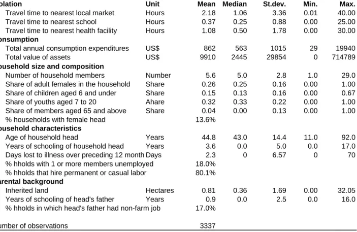
Household characteristics are summarized in Table 2. The Nepal survey contains detailed information about travel time to a number of different facilities. Given that Nepal is a very mountainous country, distance in Km is not a relevant measure for most of the country; travel time is a more accurate measure of isolation in this case. We see that, on average, surveyed households live on average more than two hours of travel time from a market, the maximum value being 40 hours.

The median is around 1 hour. Distance to local markets is the

isolation measure

that we use in our empirical analysis. Given the nature of the terrain and the spatial dispersion of households,

varies between individuals within the same ward.

Travel times to the nearest school and health facility are much shorter: on average households are located around 20 minutes from the nearest school and one hour from the nearest health facility. The quality of schools and health facilities varies widely across locations, however.

Average total annual consumption (non-durables and durables) is reported in US$.

The total value of assets is reported next. This includes land, livestock, agricultural equipment, and

and highly skewed, with the median representing around one-fourth of the mean. Parental background variables are reported as well, such as land inherited by the household, education level of the father of the household head, and whether the head’s father was employed in a non-farm occupation. Later on we use these variables to predict migration out of one’s birth ward. In 1996, towards the end of the NLSS survey, a Maoist insurgency began to take root in rural Nepal. Since the insurgency initially limited itself to attacking a few police stations,

9Our measure of isolation, ‘distance to markets’ is computed as the average of the travel time tofive different types of markets, namely market centers,hat/bazar,krishi center, cooperative center and local shops. Taking any single one of them leads to the loss of many observations. This information is recorded independently for each household.

1 0Using the exchange rate of 56.8 Rupees to the dollar which prevailed at the time of the survey. For reference, in the regression analysis we use (logged) Rupees.

it had a minimal direct impact on the welfare of survey respondents. But it may have affected their expectations regarding the future, raising the possibility of omitted variable bias. At the bottom on Table 2 we report insurgency incidence

the Nepalese police. Some 12.5% of the surveyed households resided in areas that were seriously affected by the insurgency between 1996 and 2000. These districts tend to be far from urban centers.

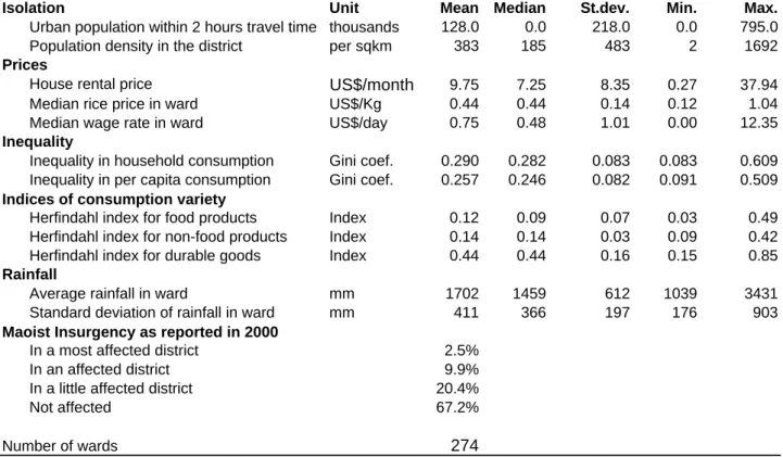
Ward-level variables are presented in Table 3. Using detailed information on the road distance between each ward and each of 34 towns and cities compiled by Fafchamps & Shilpi (2003), we construct a variable that represent the total urban population

living within 2 hours of travel distance from the ward. Population

isolation measure. Our third isolation measure is population density in the district. Other things being equal, we expect people in low population density districts to live further apart from each other, thereby raising delivery costs for private goods as well as public services.

The survey did not collect extensive price data. There is information on house rental prices, mostly on a self-assessed basis. In the next section we combine this information with house quality data to estimate a district-specific house price premium. This premium is thought to capture locational advantages reflected in housing prices. We have information on rice prices at the household level, from which we compute a ward-level median.

We use the wage rate in the ward as an additional measure of the cost of living. We compute the median wage rate in the ward from responses of individual household members. Nearly all wage employment recorded in the survey is for low skilled manual work in farm and non-farm work. We report Gini coefficients for consumption per capita computed for each ward. We use it as control. It is indeed thought

1 1Household-level prices capture differences in quality, quantity and convenience between households facing the same market. It is more reasonable to assume that all households residing in the same ward face the same prices.

Because of the presence of outliers (probably due to measurement error), we use the median price in the ward rather than the mean.

that inequality affects subjective well-being negatively. If inequality is stronger in urban areas, this could generate an omitted variable bias.

To capture the impact of product variety

, we construct for each ward indices of variety for food, non-food, and durables. For each household, the survey collected consumption expenditure information on 67 separate food items, 58 non-food items and 16 durable goods items. Based on this information, we compute the total expenditures

by all surveyed households in a ward on item

in the questionnaire, some wards consume 63 items while others only consume 33. Based on this information, we compute, for each of our three groupings

(food, non-food, and durables), a Herfindahl concentration index defined as:

N^J = S

i∈Js²_i [S

i∈Js_i]²

This index gives a rough idea of what is available for sale in the ward: the higher its value, the more concentrated spending is on a small number of categories, and the less diversified ward consumption is.

does not, however, measure product diversity within each sub- category and is thus an imperfect measure of variety. Index values reported in Table 3 show more concentration in durable expenditures and less in foodstuffs.

Two sets of dummies control for climatic and economic factors: ecological belt dummies and regional dummies. Ecological belt dummies divide the country into three North-South zones based on elevation. The mountain zone is the part of the country located at 4000 meters (12000 feet) of elevation and above. The Terai is the narrow plain bordering India. The Hills is the

1 2To the extent that richer consumers buy a greater variety of products, our variety indices are correlated with consumption expenditures. This is not a cause for concern, however, since we control for consumption expenditures directly in the regression analysis.

1 3N^J = 1 corresponds to complete concentration in a single item while N^J = 1/J corresponds to equal expenditure shares for allJ items in a category.

intermediate zone where much of the Nepalese population lives. Regional dummies capture an East-West division of the country. The Central region is where the capital Katmandu is located.

We also use average rainfall and rainfall variability between years as additional proxies for local agro-climatic conditions.

4. Econometric results

We now turn to the econometric analysis. Responses to subjective adequacy questions — coded from 1 to 3 — are the dependent variables used in our analysis. There are six dependent variables:

satisfaction with food, clothing, housing, schooling, health care, and total income. Satisfaction with total income should, in principle, combine all the effects of isolation and can be taken as proxy for

while answers to questions about specific consumption groups proxy for

. It is, however, conceivable that respondents regard monetary issues as separate from problems of product variety (N ) and access to amenities (A). Someone may, for instance, answer that his income is adequate but complain that he cannot buy the clothing or health care he desires because it is not available locally.

If, for most respondents, product variety and access to public services are conceptually distinct from the magnitude of monetary income, answers to the income adequacy question may fail to include the effects of

and

— and thus be less sensitive to isolation.

4.1. Non-parametric analysis

We begin with non-parametric univariate regressions of answers to income and consumption adequacy questions on the log of distance to markets. The purpose of the exercise is to document

1 4To an economist it would seem that a sufficiently high income would enable someone to overcome insufficient access (e.g., by paying a private tutor or paying someone to buy the clothes in town). According to this reasoning, insufficient access is ultimately an income problem. This is probably not how most respondents see it. Having a private doctor or tutor, for instance, is not within their frame of reference. It is therefore likely that, for most respondents, issues of access are distinct from issues of monetary income.

the existence of a strong correlation between the two and to illustrate that the relationship between adequacy responses and

is approximately linear.

Results are presented in Figures 1a to 1f, using an Epanechnikov kernel with moderate smoothing. The 95% confidence interval is also reported to facilitate inference.

It is immedi- ately apparent that subjective consumption adequacy falls dramatically and significantly with distance from markets.

The relationship between

and subjective adequacy is monotonic and basically linear, except at high market distances for which the small number of observations does not allow precise estimation. This means that subjective adequacy falls rapidly at short distances, before tapering off. In the rest of the analysis we use

as regressor.

As explained in the conceptual section, the relationship depicted in Figures 1a to 1f could be the result of selection by ability. To investigate this possibility, we perform a non-parametric regression of consumption expenditures on distance. For the regression to be meaningful, we need to control for differences in household size and composition. One approach would be to divide total expenditures by the number of household members, possibly weighted by gender and age, yielding consumption per adult equivalent. But doing so may bias results due to economies of size in household production (e.g. Deaton & Paxson 1998, Fafchamps & Quisumbing 2003).

To avoid such bias, we use a semi-parametric regression of the form:

logXjk =β₁B_jk+β₂logp_k+ϕ(logd_jk) +ε_jk

(4.1)

where

is a vector of controls for household

in location

and

is an arbitrary smooth function. The composition of the household is captured by the number of household members, a female head dummy, and the shares of women, young children, youth, and elderly members

1 5The 95% confidence interval for observation iis calculated as 1.96 times the robust standard error of the intercept in the local kernel regression centered on observationi.

1 6Virtually identicalfigures obtain if we use only non-migrant households.

in the household.

We also include the age and age squared of the head and we controls for price differentials to the extent allowed by the data. Prices controls include the ward median rice price, the ward median wage, and regional dummies.

The estimated function

is depicted in Figure 2. Results confirm the existence of a strong negative relationship between isolation and consumption expenditures. This

be due to sorting on ability across locations, as discussed in the conceptual section, or it could be because isolation from markets offers fewer income earning opportunities. Since consumption is lower in isolated households, this could explain lower reported satisfaction level. It is therefore important that we control for expenditures when measuring the relationship between isolation and subjective welfare.

4.2. Multivariate analysis

We now turn to a multivariate analysis. We begin by estimating an empirical equivalent of equation (2.3):

W_jk^h =f(α^h₀+α^h₁logX_jk+α^h₂logd_jk+α^h₃logP_k+α^h₄D_k+α^h₅logp_k+α^h₆B_jk)

(4.2)

where

denotes the satisfaction rankings discussed earlier and

is an ordered probit density function. Our

. Urban population within two-hour travel time from the ward,

, and population density in the district

are included as additional measures of isolation: households living in sparsely populated districts on average live further away from each other. In equation (4.2), coefficients

and

proxy for the combined effect of amenities, product variety, and local public goods.

As in (4.1), controls

are included to correct for differences in household size and composi-

1 7Adult males are the omitted category.

tion. Household size is expected to reduce income and consumption adequacy because the same level of expenditures should yield less satisfaction if the household is larger. The age and gender composition of the household may also affect how much satisfaction is derived from a given level of consumption expenditures.

Age is included to allow for life cycle effects: we expect young people to be less satisfied with life in general if their expectations are inflated by the prospect of economic growth. We expect the female head dummy to have a negative coefficient because many female headed households result from divorce and separation. The log of the value of household assets is included as additional regressor to capture permanent income effects hidden by a transitory rise or fall in expenditures. Assets may also affect subjective well-being directly through the sense of security they provide (e.g. Deaton 1991).

The median rice price and wage rate in the ward are included as price controls. We also include a district-specific housing price premium. This is estimated by regressing the (log of the) monthly rental price on district dummies, controlling for a variety of house characteristics such as square footage, number and type of rooms, quality of materials, and in-house amenities.

District dummies are thought of as capturing locational attributes such as access to public amenities and the like. We therefore expect subjective welfare to increase with the locational premium.

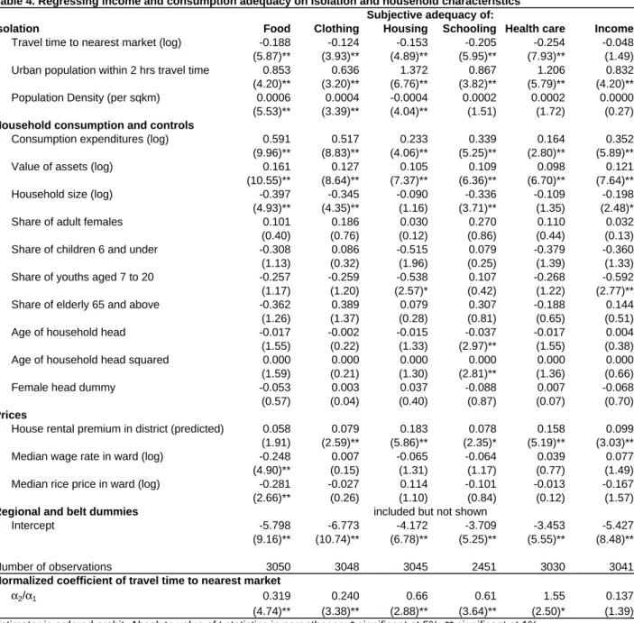
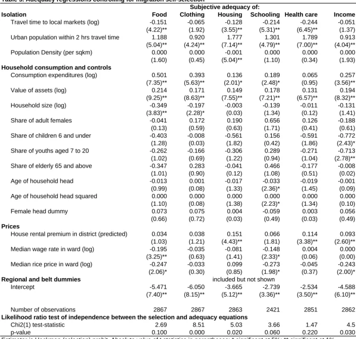
Multivariate regression results are presented in Table 4 using ordered probit.

All regressions show a negative effect of distance to markets

on subjective satisfaction. The effect is strong

1 8In particular, we note that female members typically produce services (such as home care, knitting, and sewing) which are consumed by the household (Fafchamps & Quisumbing 2003). Because it is extremely difficult to impute a value on such services, they are omitted from consumption expenditures. Adult males, in contrast, typically focus on self-employment or wage work. The monetary income they bring is properly measured as part of consumption expenditures. For this reason, we expect the share of female members in the household to raise subjective well-being once we control for consumption expenditures. These effects are captured by the share of various age/sex groups in the regression.

1 9We could in principle achieve a gain in efficiency by estimating all six regressions as a seemingly unrelated system of regressions, thereby allowing errors to be correlated across equations. Given that dependent variables are categorical, this would require six levels of numerical integration — a feat of computer programming that is not justified by the anticipated efficiency gain.

and significant in

second measure of isolation

is positive and strongly significant in all six regressions. If we omit

from the income regression, the coefficient of

is significant. Taken together, these results imply that, after controlling for consumption expenditures and household composition, subjective satisfaction is higher in households located close to markets and in or nearby large urban centers. It is not just distance to local markets that matters, but also the size of the urban population in nearby towns. Our third measure of isolation, population density

, is positive and significant at the 10% level or better in four of the six regressions, further confirming the relationship between subjective welfare and isolation. Population density, however, has a negative and significant effect on housing adequacy. This is probably due to a price effect as population concentration raises rents and house prices.

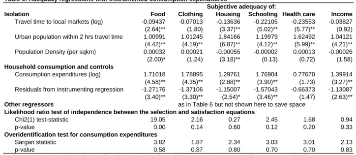
Taken together, these results indicate that subjective welfare is negatively correlated with isolation even after factoring out the effect of lower consumption expenditures. The regression results also shed some indirect light on the nature of isolation-welfare relationship. Normalized distance coefficients

are reported at the bottom of Table 4 together with their

Results indicate that the relative magnitude of the distance coefficient is largest for health care and, to a lesser extent, for schooling and housing. This is probably because households living in isolated wards

that access to public services may be a large component of the cost of isolation.

We also

consumption than for the income question itself. This suggests that answers to the income

adequacy questions do not fully capture the non-monetary costs of isolation, such as lower

product variety and access to public services. If this interpretation is correct, it follows that

most welfare costs of isolation are non-monetary. We revisit this issue in the next section.

Turning to other regressors, most controls have the anticipated sign. We

and significant coefficient of consumption expenditures in the regressions for all income and consumption adequacy questions. Household assets have a significant positive coefficient in all six regressions while household size has a significant negative coefficient in most of them. These results are consistent with the utility model. In most cases, household size and consumption expenditure have roughly the same coefficient, except with a different sign. Results would thus not change much if we simply divided consumption by the number of household members instead of entering both regressors independently.

The locational housing price premium has the anticipated positive sign and is significant in all regressions. We also note that the distance coefficient is larger when the housing price premium is omitted from the regression, suggesting that some of the effects of isolation are captured by the housing price variable. Other village-level prices have a negative and significant effect on satisfaction from food consumption, but in other regressions the price variables are mostly non-significant. We also

households located in the Mountain and Hills zone tend to report lower levels of satisfaction.

This is again consistent with other isolation results: the steeper the terrain, the less likely travel is to take place on motorized vehicles, and the more arduous travelling to the market becomes.

4.3. Possible self-selection bias

The utility approach does not depend on whether people are mobile or not — and hence is

not affected by selection across locations according to ability. But there may be unobserved

individual characteristics other than ability that influence subjective utility and are correlated

with distance. For instance, it is conceivable that there exist ‘grumpy’ people who tend to be

less intrinsically happy. As they are less sociable, they self-select into remote locations. This is

a potential source of bias.

Since the bias arises from self-selection, mobility is at the heart of the econometric problem:

among people who cannot move, there should be no systematic relationship between ‘grumpiness’

and isolation as long as grumpiness is a randomly distributed human trait. In our data, 80% of the surveyed heads of household reside in their birth ward. This suggests a strategy for dealing with potential self-selection bias. We estimate equation (4.2) using only non-migrant households and correct for self-selection into migrant status as follows:

W_jk^h = α^h₀ +α^h₁logX_jk+α^h₂logd_jk+...+u^h_jk

if

=0 (4.3)

if

= 0

if

In the country of study, male adults migrate early in life (Seddon, Adhikari & Gurung 1999).

Migrant household heads are those who were surveyed in a ward other than their birth ward.

The regressors

are variables affecting the decision to leave one’s birth place. They include predetermined individual characteristics such as education of the head and parental education.

Inherited land is included as well because it is tied to location specific knowledge that would

be lost if the household were to move. Date of birth is included to reflect changes in migration

opportunities over time. Ethnicity dummies are included in case certain groups have better

networks with migrant populations elsewhere (e.g. Seddon, Adhikari & Gurung 1999, Munshi

2003). In the following sub-section we also include ethnicity dummies and education of the

household head as additional controls in the subjective welfare regressions. Inherited land and

education and occupation of the father thus serve to identify the selection equation. They are

reasonable instruments for our purpose since they are likely to affect the migration decision but

unlikely to affect ‘grumpiness’ per se.

Model (4.3) is estimated using the bivariate probit selection estimator of Heckman. To this effect, we recode answers to the satisfaction question into two categories only — less than adequate, and adequate or more than adequate. This entails a loss of information but since the number of observations in the ‘more than adequate’ category is very small, the loss of information is minimal.

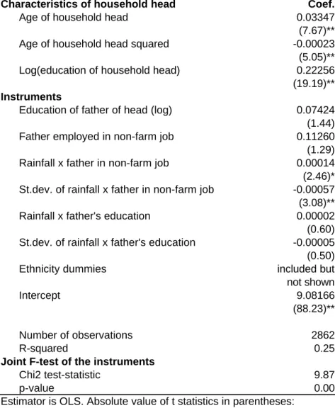
The selection regressions are presented in Appendix.

They show that better educated heads of household are significantly less likely to have remained in their birth ward. This is consistent with empirical evidence showing that returns to education are highest in non-farm activities (e.g. Yang 1997, Fafchamps & Quisumbing 2003). We also

is more likely if the head’s father is better educated, possibly reflecting an interest in off-farm work from an early age. In contrast, households inheriting a lot of land from their parents are less likely to have migrated out of their birth ward. These two variables are strongly significant, confirming that the selection equation is identified. Several ethnic dummies are also significant, with those belonging to the Brahmin caste and to the Magar and Tharu tribes more likely to migrate.

Regression results for

are presented in Table 5. Using a likelihood ratio test, the absence of correlation between the errors in the selection and satisfaction regressions is only rejected for the food regressions — but it would be rejected at

care. A selection correction is thus appropriate. As is clear from Table 5, our main results regarding isolation are basically unchanged: distance is significantly negative in all regressions except total income. The consumption expenditure variable remains positive and significant except for health care, where it is now non-significant. Other qualitative results survive as well.

2 0Since the selection and adequacy regressions are estimated jointly, there is one selection regression per ade- quacy regression. Estimated coefficients are very similar across regressions.

Thus, although a selection correction may be appropriate in this case, self-selection does not appear to be responsible for our

4.4. Robustness checks

The theoretical model presented in Section 2 suggested that isolation may affect welfare through various channels, such as prices

services

. Unfortunately we only have partial information about these channels. In Tables 4 and 5 we have already made use of the limited price information available. The results have shown that, as predicted by theory, subjective satisfaction with food consumption is lower when the local price of rice is higher. In contrast, our housing price index has a positive — and often significant — coefficient in all regressions, suggesting that the variable proxies for various locational advantages. This

land prices to fall with isolation in Nepal.

We now include additional variables that proxy for

and

the (log of the) distances from the household to the nearest school and health facility. If the relationship between isolation on subjective welfare is driven by differences in access to schools and health care, introducing these variables in the regression should result in a zero coefficient of isolation variables

and

— especially in the schooling and health care regressions.

As proxy variables for

, we use the three indices of variety

discussed in the data section.

Although imperfect, these measures give an idea of the number of distinct categories of products and services available to ward residents.

To minimize the risk of omitted variable bias, we also add a number of regressors thought to

affect subjective welfare. We begin by adding the education of the household head. Education

has been shown to influence responses to subjective welfare questions (Diener, Suh, Lucas &

Smith 1999). Unemployment and illness are included for similar reasons. The Gini coefficient of consumption per capita in the ward is included to capture possible aversion to inequality.

Rainfall in the year preceding the survey and the ward-specific standard deviation of rainfall in the year of the survey are included to capture possible effects of climate on residents’ mood.

To capture possible effects of the Maoist insurrection on people’s expectations, we include our insurgency dummies.

To control for social status we include ethnic dummies. Finally we include a dummy variable taking value 1 if the household hired permanent or casual workers in the year of the survey. The rationale for doing so is that households employing other people may feel they enjoy a higher status, and this may affect their response to adequacy questions.

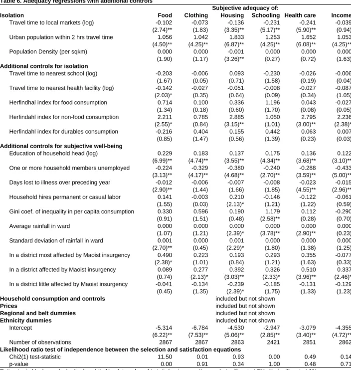
Results with the additional regressors are summarized in Table 6. A selection correction is conducted in the same way as before but not shown here to save space.

Additional controls for isolation fall short of expectations. Distance to the nearest school and health facility are never significant, suggesting that differences in physical distance to these facilities do not account for the relationship between isolation and subjective welfare. Other dimensions of local public service provision probably matter more, such as the quality of the school or health facility and the availability of drugs and teachers, for which we do not have data.

Indices

of product variety are significant in a number of regressions — mostly the index of non-food consumption. We take this as evidence that product variety is valued by Nepalese households. However, the effect of the inclusion of these variables on the distance coefficients is

2 1Admittedly, the information at our disposal measures the incidence of the insurgency four years after the survey. However, it is likely that over time the insurgency got strongest in the areas in which its action was already perceived in early 1996 when actions started. Insurgency dummies can thus be seen as an effort to capture the insurrective mood of the population in 1996.

2 2Adding this variable may also clarify the effect of the wage variable since it is likely to differ if the household is a buyer or seller of labor.

2 3After including of the additional regressors, the null hypothesis of no correlation between the error terms in the selection and satisfaction regressions can only be rejected for the food regression.

minimal, suggesting that the

indices are far from accounting for the effect of isolation.

Regarding the isolation variables themselves, our main results are basically unchanged: dis- tance remains negative and significant in all regressions except total income while urban popu- lation remains positive and significant in all regressions. Population density remains significant in two regressions. Other controls need not be discussed in detail since their inclusion is purely to eliminate possible sources of omitted variable bias.

These results demonstrate that the relationship between isolation and subjective adequacy survives the elimination of many potential sources of omitted variable bias. But they also indicate that we have not been able to identify the precise channel through which geographical isolation and subjective welfare are related.

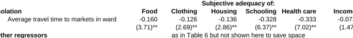
As another robustness check, we investigate whether our results may be affected by endoge- nous placement within wards. Tables 5 and 6 control for self-selection

wards. The reader may nevertheless worry about the possible endogeneity of household placement

the ward

— e.g., that grumpy people live at the outskirts of the village. To investigate this possibility, we reestimate Table 6 replacing individual distance

with the ward average

.

To save space, we show in Table 7 the regression results for the distance coefficients only. Distance is even more significant, indicating that our earlier results are not driven by endogenous placement within the ward.

We also estimate the regression including both household-specific distance to market and

2 4Education of the household head is positive and significant and unemployment is negative and significant in all regressions. Illness is negative in all regression, significantly so in five. These results are in line with experimental evidence (e.g. Frey & Stutzer 2002, Diener & Biswas-Diener 2000). Wefind that more rain tends to make people less satisfied (significant in three regressions), perhaps because rains damage roads and isolate wards further. Ethnicity variables are significant in a few regressions, usually suggesting that members of some of the tribal groups are more easily dissatisfied, perhaps because of political grievances. The labor hiring variable is marginally significant in two regressions. The Gini coefficient is significant in one regression but with the wrong sign. Maoist insurgency coefficients, when significant, usually have the wrong sign, with more affected regions appearing to be more satisfied with their income and consumption than inhabitants of least affected areas. Whatever the explanation for these results, they demonstrate that inequality and the Maoist insurgency are not what accounts for the negative relationship between income and consumption adequacy and isolation.

2 5The ward mean is computed excluding the household itself, so as to avoid spurious correlation.

average distance in the ward. Multicollinearity between the two measures gets in the way of precise estimation. The results, not presented here to save space, show that ward average distance is negative and significant at the 10% level or better in four of the six regressions. What matters most appears to be isolation of the ward itself, not relative isolation of individuals within the ward. This is further evidence that endogenous placement within the ward is unlikely to account for our results.

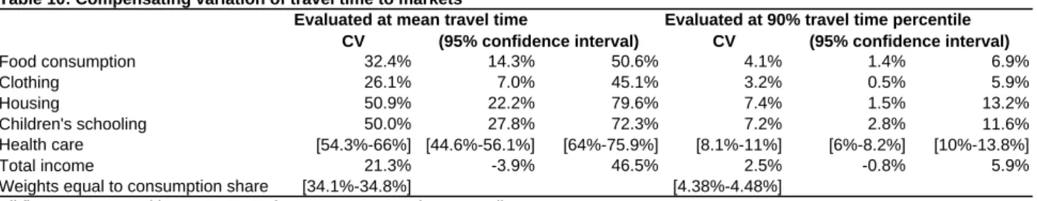
5. Magnitude

We have found a robust and significant relationship between isolation and subjective welfare. But is the magnitude of the relationship large enough to warrant further consideration? To quantify it, we draw upon the formula derived in Section 2 for estimating the equivalent variation

of reducing travel time from, say,

to

:

ckm= 1−e

α2

α1(logdk−logdm)

(5.1)

This formula provides a useful yardstick for quantifying the magnitude of the relationship be- tween

and subjective welfare.

We compute formula (5.1) replacing

and

by the coefficients of distance and con- sumption expenditures. This provides an intuitive way of quantifying the relationship between distance and welfare: if the relationship between

and subjective welfare could be interpreted as causal,

would measure the subjective cost of isolation in monetary terms.

Each of our six regressions yields separate

and

estimates and hence a different

. Differences among these

’s gives an idea of the relative magnitude of the welfare cost of isolation on different

2 6Since, for a givenlogdk−logdm,ckmis a non-linear combination of parameter estimates, a confidence interval can be computed as well.

components of utility.

The coefficient of income is not significantly different from 0 in the health care regression.

This is consistent with rationing in health care, as would be the case if health services are subsidized by government. As argued in the conceptual section, equation (5.1) is no longer valid if there is quantity rationing but we may be able to bracket

if we are willing to assume that

1

. In this case, we can use income coefficients estimated for unrationed consumption goods to normalize the distance coefficient in the rationed regression. This means calculating (5.1) with four different

and reporting the range of values found. Given that the estimated

are broadly similar across categories, we expect respondents to have answered all the adequacy questions in a comparable way.

If preferences are (approximately) homothetic, we can also compute the combined effect of isolation using

h=1ω_hV^h

where

is the consumption share of subset

can write

where

. We obtain the combined welfare cost of isolation by solving

which yields:

[H

h=1

ω_h(b + logX−λ_hlogd_k) = [H

h=1

ω_h(b + logX(1−c_km)−λ_hlogd_m)

c_km = 1−exp

# _H [

h=1

ω_hα^h₂

α^h₁(logd_k−logd_m)

$

(5.2)

where we have used the fact that consumption shares

sum to one. Equation (5.2) says that the combined welfare cost of isolation is a weighted combination of effects on consumption subsets. Because of suspected rationing in health care, we again use the bracketing method for health care, yielding a range of possible values for

.

As is clear from (5.1) and (5.2), computing the welfare cost of isolation ultimately involves

dividing the distance coefficient

by the consumption expenditure coefficient

. Estimating