Geography and Exporting Behavior

Policy Research Working Paper 5979

Geography and Exporting Behavior

Evidence from India

Megha Mukim

The World Bank

Development Research Group Trade and Integration Team February 2012

WPS5979

Public Disclosure AuthorizedPublic Disclosure AuthorizedPublic Disclosure AuthorizedPublic Disclosure Authorized

Abstract

The Policy Research Working Paper Series disseminates the findings of work in progress to encourage the exchange of ideas about development issues. An objective of the series is to get the findings out quickly, even if the presentations are less than fully polished. The papers carry the names of the authors and should be cited accordingly. The findings, interpretations, and conclusions expressed in this paper are entirely those of the authors. They do not necessarily represent the views of the International Bank for Reconstruction and Development/World Bank and its affiliated organizations, or those of the Executive Directors of the World Bank or the governments they represent.

Policy Research Working Paper 5979

This paper examines locational factors that increase the odds of a firm’s entry into export markets and affect the intensity of its participation. It differentiates between two different sources of spillovers: clustering of general economic activity and that of export-oriented activity. It also focuses on the effect of the business environment and that of institutions at the spatial unit of districts in India.

The study disentangles the within-industry effect from

This paper is a product of the Trade and Integration Team, Development Research Group. It is part of a larger effort by the World Bank to provide open access to its research and make a contribution to development policy discussions around the world. Policy Research Working Papers are also posted on the Web at http://econ.worldbank.org. The author may be contacted at m.mukim@lse.ac.uk.

the within-firm effect. A simple logit specification is used to model the probability of entry. The analysis is based on a panel of manufacturing firms in India, which allows for the introduction of firm-specific controls and a battery of fixed effects. The findings suggest that exporter- specific clustering, general economic agglomeration, and institutional factors affect firms’ export behavior.

Geography and Exporting Behavior:

Evidence from India

Megha Mukim

JEL Classification: F14, D24

Keywords: Export Entry, Extensive Margin, Intensive Margin, Economic Geography Sector Board: Economic Policy

*

London School of Economics and Columbia University; Email:

grateful to Tom Farole, Deborah Winkler, Raymond Florax, Amit Bataybal, Mark Partridge

and other participants at the Tinbergen Institute, Giovanna Prennushi and an anonymous

referee for helpful comments and suggestions. Funding from the World Bank is gratefully

acknowledged. This paper is part of a wider study on the regional determinants of trade

competitiveness conducted by the International Trade Department of the World Bank.

1 Introduction

Policy makers consider exporting to be unambiguously good – for the firm and for the economy. Although there is a lively debate about whether exporting really has a causal and positive effect on firm productivity, many national governments have set aside resources to provide domestic firms with an impetus to enter foreign markets, i.e. to start exporting. Developing countries are no different in this regard. This paper will study the decision of Indian firms to export and will analyze the factors that determine the extensive and the intensive margins of exporting. In other words, it will identify how the characteristics of a given firm, industry and location determine export participation.

In the paper export participation has been defined in two ways – the propensity of firms to start exporting, and the intensity with which they export. First, the paper tests what sorts of factors affect the probability that the firm will start to export. Factors specific to the firm, such as firm-level productivity, type, age and the size of the firm, could account for the decision to start exporting. Equally, factors specific to the industry or the location, such as agglomeration could also play a role in reducing the sunk costs of entry. In the second half of the paper, the analysis focuses on whether these factors also play an important role in affecting the performance of the firm, conditional on entry. The paper will also disentangle the cross-sectional variation across firms and the time-series variation within firms. While the former reveals how the factors of interest affect firms within a given industry, the latter reveals how these factors affect any given firm.

There are two strands of literature that are relevant to the question of sunk entry costs in exporting, and of positive externalities associated with agglomeration. Theoretical models developed by Baldwin and Krugman (1998) and Dixit (1989) describe the presence of fixed costs faced by firms to enter into export markets. These sunk costs of entry might relate to information on foreign markets, the establishment of distribution channels, the costs of complying with new or more developed product standards etc. Theoretical models have described the scope of the benefits from industrial clustering at different levels – own-industry (Marshall 1890, Arrow 1962, Romer 1986), inter-industry (Venables 1996) and through industrial diversity (Chinitz 1961, Jacobs 1969). This paper is mainly concerned with the intersection of the predictions from these theoretical models, i.e. how the presence and scope of agglomeration economies lower the sunk costs of export entry. The follow-up question is to what extent the performance of the firm is affected at the margin after entry when it continues to export.

Duranton and Puga (2004) describe microeconomic mechanisms, such as sharing, matching and learning etc., through which the benefits of agglomeration could flow to individual firms within a location

. There is also a lively empirical literature on

1

For each of these mechanisms, Duranton and Puga (2004) develop one or more core models

and discuss the associated literature. Sharing mechanisms refer to sharing individsible

facilities, sharing the gains from the wider variety of input suppliers, sharing the gains from

narrower specialisations, and sharing risks. Matching refers to mechanisms that improve

either the expected quality of matches or the probability of matching, and alleviates hold-up

measuring export spillovers. Aitken et al (1997) find that the presence of multinational firms affects the probability of entry in export markets for Mexican firms by a factor of 0.035. Becchetti and Rossi (2000) find that geographical agglomeration significantly increases export intensity and export participation (by a factor of at least 0.02) in their study of Italian firms. Greenaway et al (2004) find a similar result for firms in the UK, whereby clustering in the same region and industry increases the probability of entry by a factor of 0.016. Lovely et al (2005) find that domestic firms cluster in response to exports to countries with higher barriers to entry, suggesting the presence of export spillovers. Konig (2009) studies export spillovers by destination for French firms and finds that exporter-agglomeration positively affects the probability of starting to export to a given country by a factor of 0.14 and that these effects are destination-specific.

However, the findings of the literature are not conclusive as there are papers that find little or no evidence of export or other spillovers. Barrios et al (2003) find no evidence of export spillovers between exporters or multinationals for domestic firms in Spain, and Bernard and Jensen (2004) find no evidence that export or agglomeration spillovers affect export entry for firms in the United States.

This paper will directly test for these hypotheses to understand what factors might affect the decision of the firm to start exporting. The paper will use a panel of heterogeneous firms, wherein firms differ with regards to characteristics such as productivity, size, age and type and with regards to participation in export markets.

There are two distinct types of spillovers, (1) generated by agglomeration of more general economic activity within a location, and (2) generated by exporter-specific clustering within a location. The paper will also study the effect of the business environment more generally proxied by variables relating to levels of general infrastructure and by institutional variables. The model will control for firm and location attributes and will identify the effect of factors specific to the firm, those associated with Krugman’s (1991) first and second-nature geography

and the general investment climate. The empirical analysis is carried out using districts as a geographical unit of study – equivalent to a county in the US or in China, a unit that coincides reasonably well with Marshall’s notion of agglomeration.

The remainder of the paper is organized as follows: The next section provides a descriptive overview of the clustering of economic activity, general and export- oriented, across districts in India. Section 3 outlines the theoretical model and the estimation framework. It also describes the variables used and lists the sources of data. Section 4 presents the results of the model, for the extensive margin and Section 5 for the intensive margin of export participation. Section 6 concludes and discusses the contributions, limitations and implications of the findings.

problems. And learning refers to mechanisms based on the generation, diffusion and the accumulation of knowledge.

2

First-Nature geography is when the characteristics of the natural geography determine

clustering, and second-nature geography is when interactions between economic agents and

increasing returns to scale determine clustering.

2 Descriptive Analysis

An important focus of this paper is to ascertain what part of firms’ exporting behavior can be explained by the effect of agglomeration, in other words, if spillovers between firms can lower the sunk costs of export entry. In fact, whilst this study will also focus on the effect of various infrastructure and institutions within a location, at this stage it is pertinent to establish if there is any evidence of clustering. At a later stage, the analysis will focus on trying to disentangle the effects of second-nature effects from the natural geography and the more general sources of business-oriented advantages.

There are two phenomena that would indicate that agglomeration and exporting go hand-in-hand – if exporters were drawn to other exporters, and/or if exporters were drawn to industrial activity more generally. Different methods can be used to ascertain whether firms are uniformly distributed across various locations in the country, or if they show patterns of spatial concentration. Clustering in its simplest form can be shown through a bird’s eye view of where economic activity is located.

In this paper I look at the location of firms at the level of the district

. In particular, I compute (1) all firms, exporting and non-exporting, as a percentage of the population

and (2) firms that export as a percentage of the population. It should be kept in mind that the sample of firms contains mostly medium and large-scale manufacturing units.

In other words, I look at clustering of all firms and that of exporters after having controlled for the size of the district.

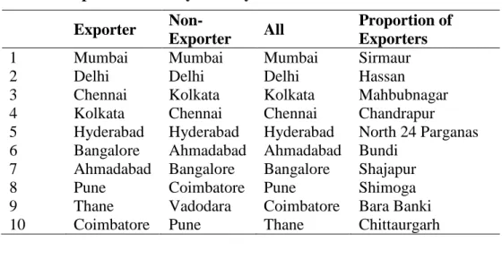
I find that there is much concordance between the districts hosting general and export- oriented economic activity. Not only do firms and exporters show evidence of clustering in a few districts, they also seem to cluster in the same districts. Table 1 lists districts in descending order of the economic activity hosted. Thus, while economic activity, whether exporting or not, seems to be located in the same districts, there is evidence of some locations hosting much higher proportions of export- oriented activity.

Having established that there is evidence of clustering of exporters and economic activity in the country, this paper will now examine to what extent the characteristics of the location affect the propensity of firms to start exporting and other attributes of their exporting behavior more generally. The effect of second-nature clustering will be identified separately from that of first-nature geography and the investment climate. The latter are particularly interesting, in so far as public policy makers can directly affect the provision of infrastructure and affect institutional variables within a location. The next section will provide a brief overview of the theoretical literature and outline a few empirical studies of relevance.

3

Maps can be made available on request.

4

Proportions instead of absolute counts are presented since it could be argued that clustering

in these districts is simply a factor of the size of the district.

Table 1: Top 10 Districts by Activity Exporter Non-

Exporter All Proportion of Exporters

1 Mumbai Mumbai Mumbai Sirmaur

2 Delhi Delhi Delhi Hassan

3 Chennai Kolkata Kolkata Mahbubnagar

4 Kolkata Chennai Chennai Chandrapur

5 Hyderabad Hyderabad Hyderabad North 24 Parganas 6 Bangalore Ahmadabad Ahmadabad Bundi

7 Ahmadabad Bangalore Bangalore Shajapur

8 Pune Coimbatore Pune Shimoga

9 Thane Vadodara Coimbatore Bara Banki

10 Coimbatore Pune Thane Chittaurgarh

3 Estimation Framework

3.1 Econometric Model

The decision to start exporting is estimated using a Logit model that controls for the specific characteristics of firms, locations and years. Consider a firm



i that makes a decision to start exporting. The associated profits are





and the sunk cost of entering export markets is



f

. Since I am mainly interested in firms that begin to export for the very first time, in this model I do not consider firms that continue to export. Because there is no need to account for export experience of a given firm, this approach has the added benefit that there is no endogeneity bias owing to the introduction of lagged export status (see Roberts and Tybout 1997, and Bernard and Jensen 2004).

Following Konig (2009) it is assumed that a firm will start to export if profits associated with entry exceed the cost of entry, i.e.





 f

. Thus, the probability that a firm



i starts to export at time



t is given by:



Pr( Y

1)  Pr( 

 f

) (1)

Profits of a firm are assumed to be a function of productivity and other characteristics of the firm, and the sunk cost of entry is assumed to be a function of local exporting activity and agglomeration specific to a given industry (



k ) in a location (



j ).

Rewriting Equation (1), the probability of starting to export is given by:



Pr( Y

 1)  Pr( 

X

 

Z

 

 0) (2) where firm characteristics are included in the vector



X

, and characteristics affecting the sunk cost of entry specific to the location and industry are included in



Z

. This

expression can be estimated using a Logit model under the assumption that the error

term is distributed logistically. Thus, the dependent variable Y

is a dummy variable

describing whether the firm



i starts to export at time period



t . The regressions include only those firms that have entered the export market at least once – in other words, firms that have never export over the sample period are excluded.

Additionally, the dependent variable equals 1 for the year in which the firm first starts exporting and equals 0 for all other years leading up to that year. If firms continue to export, or if they switch status after having entered the export market for the first time, these observations are not included in the regressions.

3.2 Specification of Variables

The deterministic component of the function consists of the various attributes of the location that can influence the propensity of a firm to start exporting. The random component consists of the unobserved characteristics of the location and measurement errors. As mentioned above, the dependent variable is a dummy variable at time



t that equals 1 if the firm starts to export and 0 for all years leading up to



t . The explanatory variables in the model are defined at time



t  1 , and as indicated, for National Industrial Classification (NIC) 2-digit industry (



k ) and at the spatial unit of the district (



j ) or the state (



J ). The sources of data are described later in Section 3.3.

Firm-specific characteristics include 

, which represents the productivity of the firm,



age

, which represents the age of the firm, size

, which represents the size of the firm, and



type

, which represents the type of firm (private domestic, private foreign, public or mixed). Agglomeration (or, second-nature geography) are described by



exp

, which represents the count of other exporters found in district



j weighted by district population, exp

, which represents the count of other exporters by industry found in district



j weighted by district population,





, which represents localization economies, represented by the share of employment in industry k found in district j,





, which represents inter-industry trading relations measured by the strength of buyer-supplier linkages, and



U

, which represents urbanization economies in district j. Other economic geography variables getting at first-nature geography include



MA

, which summarizes access to markets in neighboring districts, and Port

, which summarizes distance for a given district from the closest port.

Infrastructure variables are given by



Road

, which measures the density of roads (primary and secondary) in district j,



Ed

, which measures the level of human capital in district j,



X

, which captures the quality and availability of infrastructure (electricity and communications),



W

, which is a vector of factor input price variables in district j, and



WE

, which captures the level of wealth in district j. And lastly, institutional variables are given by



flex

, which is an indicator of the flexibility of labor regulations in state



J , and



riots

, which is an indicator of social institutions and unrest.

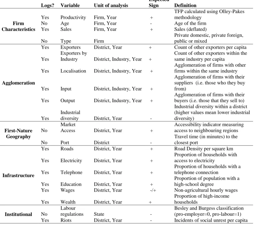
The remainder of this section provides a detailed description of each of the variables

used in the model – firm-specific variables, second-nature geography, first-nature

geography, infrastructure and institutional. For easy reference, a summary of the variables is provided in Table 2.

Firm-Specific Controls

Firm-specific controls include the productivity, size (sales), age and the type of firm (private domestic, private foreign, public or mixed). The literature suggests that exporters are usually more productive than non-exporters because of two distinct mechanisms - self-selection into export markets and learning-by-exporting. Exporters may be more productive than their counterparts, who only supply the domestic market, simply because more productive firms are able to engage in export activity and compete in international markets. The second mechanism is post-entry productivity benefits, since when firms enter into export markets they gain new knowledge and expertise, which allows them to improve their level of efficiency.

While this paper is not concerned with the casual impact of exporting on productivity, it is important to control for the self-selection of more productive firms into exporting. Lagging productivity by one period effectively controls for possible endogeneity, since the decision to ‘start’ exporting takes place only once.

To obtain consistent production function estimates, this paper follows Olley and Pakes (1996) to compute firm-level total factor productivity (





). This approach controls for two distinct sources of bias (1) simultaneity between outputs and inputs, which would bias the labor coefficient upward and (2) endogeneous exit of firms from the sample, which would bias the capital coefficient downward. Under fairly general assumptions, Levinsohn and Petrin (2003) show that with simple OLS estimations the labor coefficient will be upward biased and the capital coefficient will be downward biased. This would imply that productivity estimates would be upward biased for more capital-intensive firms, such as exporters. I compute the labor and capital coefficients under simple OLS assumptions and using the Olley-Pakes procedure and report these in Appendix Table A.1. I use data on the firm’s total wage bill as a proxy for the labor input, and on its fixed assets

as a proxy for capital. These nominal values are deflated using NIC 2-digit level output and input specific price indices

. Agglomeration Variables

The count of other exporters within the district ( exp ) and the count of other

exporters by industry within the district ( exp

) are weighted by the district population captures the effect of export spillovers. The idea is that proximity to other exporters could result in knowledge spillovers that might help non-exporters to start exporting. In addition more general industrial agglomeration within a location would

5

Fixed assets include plant and machinery, computers, electrical installations, transport and communication equipment and infrastructure, fittings and furniture, social amenities and other fixed assets.

6

Since more productive forms are likely to have a lower-than-average firm specific price, the

use of industry price indices might systematically underestimate the output of more

productive firms and therefore underestimate their productivity. On the other hand, if

exporters were more likely to use better quality inputs and materials, then using industry-

specific deflators would overestimate productivity. The converse would be true for less

productive firms. In the absence of firm-specific prices I am unable to overcome this bias.

also increase the likelihood for denser interactions between exporters, no matter what the proportion of exporters in the overall cluster. Thus, not only does the specification control for the effect of other exporters, by industry and otherwise, within a district, it also includes measures of own-industry and input-output agglomeration and industrial diversity. It should be noted that clustering could also be associated with diseconomies such as congestion or increased competition. Thus, the estimations will capture the net effect of the positive and negative impacts on export participation.

Localization economies ( 

) can be measured by own industry employment in the district, own industry establishments in the district, or an index of concentration, which reflects disproportionately high concentration of the industry in the district in comparison to the country. I measure localization economies as the proportion of industry



k ’s firms in district



j as a share of all of all industry



k firms in the country for a given year t. The variable takes a different value for each industry in a given district, across districts. It identifies spillovers that are associated with within-industry clustering, regardless of the final markets that these firms serve. The higher this value, the higher the expectation of intra-industry concentration benefits in the district.

kt jkt

jkt

E

 E



There are several approaches for defining inter-industry linkages: input-output based, labor skill based and technology flow based. Although these approaches represent different aspects of industry linkages and the structure of a regional economy, the most common approach is to use the national level input-output accounts as templates for identifying strengths and weaknesses in regional buyer-supplier linkages (Feser and Bergman 2000). The strong presence or lack of nationally identified buyer- supplier linkages at the local level can be a good indicator of the probability that a firm is located in that region. To evaluate the strength of buyer (supplier) linkages for each industry, a summation of regional (here district) industry firms weighted by the industry’s input (output) coefficient column (row) vector from the national input- output account is used:







k

jkt k

jkt

w n

1

where,





is the strength of the buyer (supplier) linkage,



w

is industry k’s national

input (output) co-efficient column (row) vector and n

is the total number of firms in

industry k in district j in year t. The measure examines local level inter-industry

linkages based on national input-output accounts. The national I-O coefficient column

vectors describe intermediate goods requirements for each industry, whilst the I-O

coefficient row vectors describe final good sales for each industry. Assuming that

local industries follow the national average in terms of their purchasing (selling)

patterns of intermediate (final) goods, national level linkages can be imposed to the

local level industry structure for examining whether district j has a right mix of buyer-

supplier industries for industry k. By multiplying the national I-O coefficient vector,

which is time-invariant, for industry k and the size of each sector in district j, simple

local firm numbers can be weighted based on what industry k purchases or sells nationally.

I use the Herfindal measure to examine the degree of economic diversity in each district. I refer to this measure as urbanization economies ( U

) in each district in a given year t. Urbanization economies are a reference to large urban areas, which are industrially diverse, which enjoy access to large labour pools with multiple degrees of specialization, access to financial and professional services, better physical and social infrastructures etc. The Herfindahl Index, although it captures only the level of industrial diversity within a region, is a proxy for these larger urbanization economies. The Herfindal Index of a district j ( U

) is the sum of squares of firm shares of all industries in district j:

2

 _ ^





 



 

k jt

jkt

jt

E

U E

Unlike measures of specialization, which focus on one industry, the diversity index considers the industry mix of the entire regional economy. The largest value for



U

is one when the entire regional economy is dominated by a single industry. Thus a higher value signifies a lower level of economic diversity.

First-Nature Geography Variables

In principle, improved access to consumer markets (including inter-industry buyers and suppliers) will increase the demand for a firm’s products, thereby providing the incentive to increase scale and invest in cost-reducing technologies. The proposed model will use the formulation proposed initially by Hanson (1959), which states that the accessibility at point A to a particular type of activity at area B (say, employment) is directly proportional to the size of the activity at area B (say, number of jobs) and inversely proportional to some function of the distance separating point A from area B. Accessibility is thus defined as the potential for opportunities for interactions with neighboring districts and is defined as:





j b

m j

mt

jt

d

MA S

Where, MA

is the accessibility indicator estimated for location j in year t,



S

is a size indicator at destination m (in this case, district population) in a given year,



d

is a measure of distance between origin j and destination m, and b describes how increasing distance reduces the expected level of interaction

. The size of the district of origin



j is not included in the computation of market access – only that of neighboring districts is taken into account. Thus, the accessibility indicator is constructed using population (as the size indicator), distance (as a measure of separation) and is estimated without exponent values. The measure of distance is

7

In the original model proposed by Hanson (1959), b is an exponent describing the effect of

the travel time between the zones.

travel-time distance (in number of minutes) connecting any given pair of districts.

Origin and destination points are located at the geographic center of each district, and the travel-time estimate is based on the least time-consuming path between the two.

Time is computed

using Geographic Information Systems (GIS) as the length of the road between two points with assumptions about the speed of travel according to different road categories

. The same travel-time measure is also used to compute Port

, the distance of a given district to the closest of the 13 largest trading ports in the country. Access to a major merchandise chipping port should, in theory, positively impact the probability of starting to export.

Infrastructure Variables

The next set of variables deals with the general quality of infrastructure within a district, since one would expect that the general business environment would have a positive impact on the probability of a firm to enter export markets. Such variables are also particularly interesting to policy makers since, unlike agglomeration, targeted investments within a location can help to improve infrastructure and make a location more business-friendly. I include the density of roads, i.e. the length of roads per square kilometer within a district, as a proxy for transport infrastructure. I computed these values using ArcGIS data, and the density data is time-invariant

. I assess quantitatively the role played by human capital by including the proportion of the population within the district with a high-school education in a given year, captured by the education variable - Ed

. I define X

as a measure of ‘natural advantage’

through the embedded quality and availability of infrastructure in the district. I use the availability of power (proxied by the proportion of households with access to electricity) within a location as an indicator of the provision of infrastructure. In addition I also use the proportion of households within a district with a telephone connection as an indicator of communications’ infrastructure.

W

is an indicator of labor costs in location j, and is given by nominal district-level wage rates (i.e. non-agricultural hourly wages). The expected effect of this variable is hard to pin down theoretically. On the one hand, if wages were a measure of input costs then one would expect export activity to be inversely related to wages.

However, it is also important to control for the skill set of the workers since a positive coefficient on wages could be a proxy for more skilled labor. Although I am unable to directly control for the ability of the worker, I include ‘education’ as a proxy for the level of human capital within the district. And thus, the proportion of high-income households ( WE

) within a district is an indicator of the general level of wealth, or more specifically, consumer expenditure within a district. The variable is constructed

8

The author is grateful to Brian Blankespoor of the World Bank for carrying out the computations and for making the data available for this analysis.

9

Some examples of road types are motorways, primary roads, secondary roads, trunk links, tertiary roads, residential roads etc.

10

This is a strong assumption, and with the availability of better data the paper will attempt to

update these results at a later stage.

using household consumption data and refers to those households that belong to the highest monthly per-capita consumption expenditure group

.

Institutional Variables

I also control for the quality of institutions within the location. I include a dummy variable which is set equal to one for states with labor laws rated as pro-business by Besley and Burgess (2004). While labor regulations are mainly legislated and enforced by state governments, they also have an important effect on the cost of contracts at the district level. I also include a district-level variable on the frequency of riots and social unrest per capita across different years as a proxy for social institutions. This information is drawn from Marshall and Marshall (2008).

In summary, the firm characteristics and economic geography variables are supplemented with controls for infrastructure (transport, education, electricity and telephone), input costs (wages) and institutional variables (flexibility of labor regulations and social unrest).

11

The actual consumption category differs depending on the year of the survey, the type of

district (rural or urban) and the population of the district.

Table 2: Summary of Variables

Logs? Variable Unit of analysis

Expected

Sign Definition

Firm Characteristics

Yes Productivity Firm, Year +

TFP calculated using Olley-Pakes methodology

No Age Firm, Year - Age of the firm

Yes Sales Firm, Year + Sales (deflated)

No Type Firm

Private domestic, private foreign, public or mixed

Agglomeration

Yes Exporters District, Year + Count of other exporters per capita Yes

Exporters by

Industry District, Industry, Year +

Count of other exporters within the same industry per capita

Yes Localisation District, Industry, Year +

Agglomeration of firms with other firms within the same industry

Yes Input District, Industry, Year +

Agglomeration of firms with their suppliers (i.e. those who they buy from)

Yes Output District, Industry, Year +

Agglomeration of firms with their buyers (i.e. those that they sell to)

Yes

Industrial

diversity District, Year -

Industrial diversity within a district (higher values mean lower industrial diversity)

First-Nature Geography

No

Market

Access District, Year +

Accessibility indicator measuring access to neighbouring regions

No Port District -

Travel time (in minutes) to the closest port

Infrastructure

Yes Roads District, Year + Road Density per square km

Yes Electricity District, Year +

Proportion of households with access to electricity

Yes Telephone District, Year +

Proportion of households with a telephone connection

Yes Education District, Year +

Proportion of population with a high-school degree

Yes Wages District, Year -/+ Non-agricultural hourly wages

Yes Wealth District, Year +

Proportion of high-income households

Institutional

No

Labour

regulations State -

Besley and Burgess classification (pro-employer=0, pro-labour=1) Yes Riots District, Year - Incidents of social unrest per capita

3.3 Sources of Data

Firm-level data on export behavior (i.e. when a firm starts to export and following

entry into export markets, the value of exports as a proportion of sales) and on output

and inputs is drawn from the Prowess database. Prowess is a corporate database that

contains normalized data built on a sound understanding of disclosures of over 20,000

companies in India. The database provides financial statements, ratio analysis, fund

flows, product profiles, returns and risks on the stock market etc. The Centre for

Monitoring the Indian Economy (CMIE), which collects data from 1989 onwards,

assembles the Prowess database. The database contains information on 23,168 firms

for the year 1989 – 2008

. After cleaning the data, the final dataset contains 6,296 firms. Since there is limited data for other district-level variables, the analysis is restricted to fewer years (1999-2004). The analysis is limited to the manufacturing sector (i.e. National Industrial Classification 2-digit unit 14 to 36). I also exclude firms for which data on sales, gross assets and wages is missing, since these are crucial to the computation of firm-level productivity. Of the firms in the final dataset, 3,638 firms enter the export market at least once over the period of study. There is also a large degree of firm heterogeneity in terms of size and age.

However, some caveats should be mentioned here. It is not mandatory for firms to supply data to the CMIE, and one cannot tell exactly how representative of the industry is the membership of the firms in the organization. Prowess covers 60-70 percent of the organized sector in India, 75 percent of corporate taxes and 95 percent of excise duties collected by the Government of India (Goldberg et al 2010

). Large firms, which account for a large percentage of industrial production and foreign trade, are usually members of the CMIE and are more likely to be included in the database.

And so, the analysis is based on a sample of firms that is, in all probability, taken disproportionately from the higher end of the size distribution. As Tybout and Westbrook (1994) point out, a lot of productivity growth comes from larger plants, which are also more likely to be exporters, providing confidence in the comprehensive scope of the study.

Measures of agglomeration are constructed using unit-level data for the years 1999- 2004 from the Annual Survey of Industries (ASI), conducted by the Central Statistical Office of the Government of India. The ASI covers all factories registered under the Factories Act of 1948 that employ 20 or more workers, or that employ 10 or more workers and use electricity. Although the ASI data has a large sample size, certainly larger than Prowess, and it contains data on firm-level characteristics, it cannot be used to study firm-level export behavior. This is because even though the ASI provides information on whether a firm exports or not, the database does not follow firms over time. In other words, firms are sampled afresh every year and it is not possible to create a panel of firms over time. Data on the number of units, i.e. the plant or the factory, is used in the analysis since employment-level data is often scarce or missing. As ASI collects data for primarily the manufacturing sector, agglomeration measures do not account for the activities of services enterprises. This is a shortcoming of the analysis since service sector activity and clustering within a location might be strongly associated with the availability of essential inputs that might reduce entry costs into export markets. Data on market access is constructed using district-level population drawn by various surveys of the National Sample Survey Organisation (NSSO).

Data on measures of infrastructure, such as education, electricity and communications infrastructure, and on wages and wealth within the district are also drawn from the household surveys of the NSSO. These data are only available for 3 Rounds: Round 55.10 (July 1999 - June 2000), Round 60.10 (June 2004) and Round 61.10 (July 2004 - June 2005). The specifications with infrastructure variables thus refer to fewer years than those for firm-level and economic geography variables. And lastly, as mentioned

12

More recent data is also available, but the data extracted by the author stops at 2008.

13

Quoted in earlier version of NBER working paper.

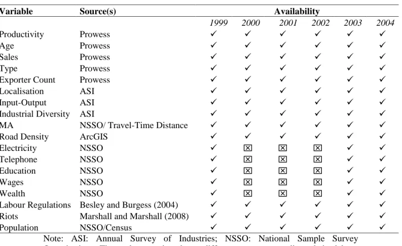
previously, Besley and Burgess (2004) and Marshall and Marshall (2008) are the main source for the data on the flexibility of labor regulations and of measures of social unrest, respectively. A tabular summary of the data is provided in Table 3.

Table 3: Data Availability

Variable Source(s) Availability

1999 2000 2001 2002 2003 2004

Productivity Prowess      

Age Prowess      

Sales Prowess      

Type Prowess      

Exporter Count Prowess      

Localisation ASI      

Input-Output ASI      

Industrial Diversity ASI      

MA NSSO/ Travel-Time Distance      

Road Density ArcGIS      

Electricity NSSO      

Telephone NSSO      

Education NSSO      

Wages NSSO      

Wealth NSSO      

Labour Regulations Besley and Burgess (2004)      

Riots Marshall and Marshall (2008)      

Population NSSO/Census      

Note: ASI: Annual Survey of Industries; NSSO: National Sample Survey Organisation. The values assigned to different states regarding their labour regulations, and those for road density assigned to districts do not vary over year, and the value does not vary over time.

4 Results: The Extensive Margin

4.1 Across Firms

The results of the econometric specification are provided in Table 4. The dependent variable is ‘start’ i.e. a dummy variable that equals one if the firm starts exporting and zero otherwise. All columns include year and industry (2-digit NIC level) controls.

From left to right, the columns present estimations that include an increasing number

of variables and then finally also include location-specific effects. Model specification

(1) controls for firm-level characteristics only; in addition to these, model (2) includes

agglomeration variables; model (3) adds first-nature geography variables; model (4)

adds further infrastructure variables, and model (5) adds institutional variables. Model

(6), which includes all variables, firm, second and first nature, infrastructure and

institutional, also includes state fixed effects. Owing to limited data availability for

infrastructure variables, as described earlier, the number of observations is considerably reduced in model (4). Due to missing data, this loss of observations is exacerbated in models (5) and (6).

As one would expect, firm-level productivity is strongly and positively associated with the decision of the firm to enter export markets, providing some evidence for self-selection of the most productive firms into the export market. Additionally, the size of the firm seems to effect the export decision negatively, suggesting that smaller firms are more likely to start exporting. Interestingly, once productivity is controlled for, the age of the firm has no statistically significant effect on the log odds of entry.

Also, once infrastructure variables are included in the regressions, these effects are no longer statistically significant.

The count of existing exporters per capita, by industry and in total, within a district seems to have little or no discernible effect on the propensity of the firm to export.

For example, the magnitude of the coefficient of ‘Exporter Count’ in model (6) can be interpreted as follows: a unit increase in the percentage of exporters within a district decreases the log odds of starting to export by 0.2857, although this variable is only significant at the 10 percent level.

Other aspects of more general agglomeration within a district, i.e. localization, input- output economies and industrial diversity have a stronger impact on the odds of entering export markets. In fact, the coefficient on localization is negative suggesting that this variable might be capturing some aspects of competition across firms within the same industry – although the coefficient is not significant in any specifications barring the one in model 4. Input linkages, i.e. access to suppliers, have a positive effect before infrastructure controls are introduced. On the other hand, proximity to buyers, i.e. those that firms sell to, seems to have a negative effect. The effect of industrial diversity is stable and negative, but statistically insignificant, across different specifications.

In Column (3) first-nature economic geography variables are introduced – market access and access to the closest port. Neither variable seems to have any effect on the probability of starting to export.

Model (4) introduces infrastructure variables into the specification, and finds that

most of these variables seem to have little or no effect on the odds of a firm entering

export markets. Interestingly however, the effect of education (i.e. the proportion of

the population with a high-school degree) is positive and significant at the 10 percent

level. In lengthier checks (not shown here) the introduction of road density reduces

the significance of the education variable, suggesting that some of the effect of more

skilled labor is explained by the availability of better transport infrastructure. Lower

wages seem to reduce the costs of entry, but the effect is not significant across

specifications.

Table 4: Decision to Start Exporting (Across-Firm Logit)

(1) (2) (3) (4) (5) (6)

Productivity 0.0840** 0.0801** 0.0789** 0.0913 0.0046 0.0125

[0.037] [0.039] [0.039] [0.130] [0.170] [0.185]

Age -0.0002 -0.0010 -0.0008 0.0024 0.0049 0.0050

[0.002] [0.002] [0.002] [0.007] [0.009] [0.009]

Size -0.1280*** -0.1303*** -0.1327*** -0.0455 -0.0256 -0.0105

[0.031] [0.035] [0.036] [0.060] [0.093] [0.104]

Exporter Count 0.0422 0.0551 -0.1350 -0.1733 -0.2857*

[0.041] [0.044] [0.103] [0.133] [0.173]

Exporter Count (Ind) 0.0275 0.0244 0.0166 0.0569 0.0971

[0.044] [0.042] [0.127] [0.142] [0.148]

Localisation -0.0019 0.0142 -0.1750*** -0.9611 -0.9169

[0.028] [0.034] [0.064] [2.046] [2.171]

Input Economies 0.3357*** 0.3423*** 0.0153 -0.5117 -0.6113

[0.123] [0.123] [0.263] [0.657] [0.693]

Output Economies -0.3609*** -0.3815*** 0.0676 1.3390 1.3776

[0.113] [0.114] [0.262] [2.673] [2.837]

Diversity -0.0577 -0.0219 -0.0247 -0.2156 -0.1450

[0.075] [0.089] [0.190] [0.234] [0.296]

Market Access 0.0000 -0.0000 -0.0000 0.0000

[0.000] [0.000] [0.000] [0.000]

Port 0.0000 -0.0003 -0.0006 -0.0005

[0.000] [0.000] [0.000] [0.001]

Road Density 0.1674 0.1720 0.2985

[0.153] [0.185] [0.317]

Telephone -0.0104 -0.0031 -0.2274

[0.219] [0.226] [0.300]

Electricity 0.3126 0.1813 0.0855

[0.470] [0.534] [0.720]

Education 0.5746* 0.4870* 0.6845*

[0.342] [0.413] [0.502]

Wages 0.1035 0.0748 0.1809

[0.555] [0.575] [0.617]

Wealth 0.0143 -0.0792 -0.2822

[0.213] [0.224] [0.255]

Flex -0.0625 0.0000

[0.288] [0.000]

Riots -0.1233** -0.1321**

[0.053] [0.067]

Population 0.0466 0.0184 -0.0488 0.0495 0.0876 -0.4675

[0.033] [0.059] [0.096] [0.241] [0.458] [0.774]

Fixed Effects

Year &

Industry

Year &

Industry

Year &

Industry

Year &

Industry

Year &

Industry

Year &

Industry &

State

# 2,519 2,300 2,272 679 478 478

Pseudo



R

0.0181 0.0192 0.0191 0.0481 0.0689 0.0753

Notes: All specifications control for the type of the firm (i.e. private domestic, private foreign,

public and mixed); Lagged values ( t  1 ) of explanatory variables are being used. Robust

Errors in brackets, clustered at the district level; *** p<0.01, ** p<0.05, * p<0.1

And finally, institutional variables at the state (i.e. the flexibility of labor regulations) and at the district (i.e. social unrest per capita) are introduced in model (5). The effect of business-friendly labor regulations is insignificant. The impact of riots per capita, however, is negative and significant suggesting that more social unrest within a district lowers the odds of a firm’s entry into export markets.

The last column (6) introduces location (i.e. state

) fixed-effects in an attempt to control for any unobserved characteristics of the location that are not captured by the first-nature geography variables. In summary, the effect of firm-specific characteristics, namely productivity and size of the firm, has a significant effect on the odds of entry into exporting. Additionally, the agglomeration of same-industry firms within a district seems to have a negative effect, although that of exporter-specific clustering within the district is harder to pin down. Access to suppliers positively effects entry, while access to buyers does not. The level of skilled labor within a location has a positive effect, and social unrest is associated with lower odds of entry.

4.2 Within Firms

The previous regressions have been estimated at the industry-level. Including industry dummies implies that the coefficients are averaged for all firms within a given industry (and year and/or state). However, it could also be the case that a change in industry-level (or state-level) characteristics could affect firms in that industry differently, depending on the individual characteristics of the firm. For instance, Bown and Porto (2010) study the effect of a change in preferential market access for the Indian steel industry and find that some firms within the industry, such as those which historically had ties to developed markets, responded more quickly than others in order to increase their exports. Indeed, as their analysis shows, aggregating variables at the industry-level fails to capture the differences across firms, some of which are large producers who were active for a number of years prior to the shock and others that were relatively new entrants to the market

. And since ultimately the analysis is concerned with studying the effect of agglomeration and other characteristics of a location on the propensity of a given firm to enter export markets, this section re-runs the regressions with the introduction of firm fixed-effects.

Taking firm-fixed effects not only constrains the coefficient to be averaged within- firms and not across firms, it also provides the most stringent control. It effectively controls for any possible endogeneity running from unobservables at the level of industries and locations, and the coefficients describe the effects at the level of firms over time. It is then redundant to take account of industry or location unobservables and the introduction of firm dummies provides a much cleaner analysis of effects at the level of the firm. Table 5 reports the results from the specifications that include

14

Convergence is not reached when district fixed-effects are introduced.

15

For instance, when aggregated across all firms, it seems that the share of sales associated

with the preferential products seems to fall in response to the increase in market access. This

could be because new entrants in the market sell only a small share of preferential products,

compared to more established firms, which brings down the aggregate average for all firms.

firm fixed-effects. Since convergence was not reached with the inclusion of infrastructure variables, the models were run without them

.

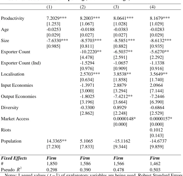
Table 5: Decision to Start Exporting (Within-Firm Logit)

(1) (2) (3) (4)

Productivity 7.2029*** 8.2003*** 8.0641*** 8.1679***

[1.253] [1.067] [1.028] [1.029]

Age -0.0253 -0.0188 -0.0383 -0.0283

[0.029] [0.027] [0.027] [0.029]

Size -7.6330*** -8.5703*** -8.5851*** -8.6132***

[0.985] [0.811] [0.882] [0.935]

Exporter Count -10.2220** -6.5037** -5.6270**

[4.478] [2.591] [2.292]

Exporter Count (Ind) -1.5294 -1.0657 -1.1338

[0.976] [0.909] [0.916]

Localisation 2.5703*** 3.8538** 3.5649**

[0.634] [1.858] [1.740]

Input Economies -1.3971 2.8879 2.0964

[3.000] [3.294] [7.144]

Output Economies -1.8025 -7.4212** -7.2446

[3.196] [3.664] [6.390]

Diversity -0.3300 0.8929 -0.6864

[2.862] [2.248] [2.529]

Market Access 0.0000148* 0.0000157*

[0.000] [0.000]

Riots 0.1012

[0.143]

Population 14.3365** 5.1065 -15.1162 -14.6737

[7.230] [7.833] [9.344] [9.859]

Fixed Effects Firm Firm Firm Firm

# 1,850 1,586 1,566 1,462

Pseudo



R

0.298 0.390 0.478 0.503

Notes: Lagged values (



t 1 ) of explanatory variables are being used. Robust Standard Errors in brackets, clustered at the firm level; *** p<0.01, ** p<0.05, * p<0.1

Controlling for all characteristics of a given firm, the size of the firm has a negative effect on its odds of entry. Just as in the earlier section 4.1 on across-firm estimations, this suggests that smaller firms are more likely to start exporting

. However, the coefficient on productivity is not only larger in magnitude, it is also highly significant across all specifications. Since productivity has been lagged, this is robust evidence to support the theory that more productive firms are more likely to self-select into exporting.

16

I also tried the model with the inclusion of firm and year fixed-effects, but convergence was not reached.

17

Keep in mind that this model says nothing about the intensity with which a firm might

export, and looks exclusively at the decision to enter the export market. The next section will

look more closely at the effect of continued and more intensive export participation.

There are some marked differences compared to the results of the across-firms analysis. The effect of clustering of exporters within the district has a strong negative and significant effect on the probability of a given firm to enter export markets. In other words, being surrounded by other exporting firms, irrespective of industry type, seems to discourage entry. On the other hand, the effects of more general industrial agglomeration are much more noteworthy than in earlier models. For instance, within- industry clustering of firms seems to have a strong positive effect on the log odds of entry into export markets. Additionally, local industrial diversity seems to have no effect on the log odds of entry. Compared to earlier results, now access to larger neighboring markets positively affects the odds that a firm will enter the export market.

Although these specifications shed much light about the effect of geography and firm-level variables on the decision of the firm to start exporting, they don’t say much about how these very variables might affect export participation conditional on entry.

The next section will explore these effects in greater detail.

5 Results: The Intensive Margin

There is evidence (Das, Roberts and Tybout 2007) to show that entry costs are substantial not just with regards to the decision to export, i.e. the extensive margin, but also with regards to how much to export, i.e. the intensive margin. Thus, it could be argued that characteristics of the location affect not only the probability that a firm might start to export, but that they also have an effect on the continued success of the firm in export markets. Firms seeking to enter foreign markets might face fixed costs of participation for every additional year of exporting. Indeed, there is some evidence (Arkolakis 2009) to show that firms begin by exporting small quantities and increase their volume of exports quickly over time. Thus, export performance could also be measured as the intensity with which firms export.

To identify the effect of geography and firm-level variables on the intensity of export participation, I regress the log of the value of exports on a set of firm, industry and location-specific characteristics, similar to those in Equation (2):

ijkt jkt it

it

 

 

X  

Z  

exp

ln (3)

Equation (3) is estimation using Ordinary Least Squares (OLS) regressions

. Firm characteristics are included in the vector



X

, and characteristics specific to the

18

I also had the choice of regressing exports of the firm as a proportion of sales on the explanatory variables. In this case the dependent variable would be a fraction that varies between 0 and 1, and using OLS would lead to incorrectly identified coefficients. This is because the effect of any explanatory variable cannot be constant through its entire range.

Additionally, the predicted values from an OLS regression often produce figures outside the

range of 0 to 1. Papke and Woolridge (1996) examine potential econometric alternatives and

support using quasi-likelihood methods. Accordingly, I try and use fractional logit

location and industry are included in



Z

. As in Section (4) above, I will identify the effects of geography and firm characteristics for firms within a given industry and location, and then for a given firm.

5.1 Across Firms

The first set of results is presented in Table 6, wherein the model specifications are the same as those in Table 4. However, the dependent variable is now the log of total exports of the firm, since I am mainly interested in understanding the factors that affect the intensity of participation in export markets.

The first striking result is that lagged productivity has a negative effect on value of exports – in fact a 1 percent increase in productivity seems to lower exports by anything between 29 to 33 percent. Age is also negatively associated with export intensity, indicating that younger firms tend to export more. And, intuitively, the size of the firm is positively associated with exports.

The clustering of exporters within the district seems to affect export intensity negatively, while the clustering of exporters of the same industry within the district has a positive effect. A percentage increase in the number of same-industry exporters within the district increases the value of exports by 16 percent. In the same vein, more general clustering, i.e. clustering of firms within the same industry, has a positive and significant coefficient. Thus, there is some evidence of positive externalities of within-industry clustering on the intensity of a firm’s participation in export markets.

Access to suppliers has a positive effect, and access to buyers has a negative effect, although these coefficients are not statistically significant once infrastructure and other variables are controlled for.

Market access has a negative effect, although the magnitude of the effect is small.

Access to the closest port has a negative effect suggesting that firms closer to large trading ports are more likely to export more. In fact a 1-minute increase in the travel- time distance to the closest port decreases exports by 0.11 percent (see model 6). It seems that being located close to a port does not affect the odds of starting to export (see the result in Table 4) but that it does positively affect the intensity of export participation. Firms close to a large trading port are not more likely to start exporting, but once they do start exporting they are more likely to export more.

Infrastructure variables seem to be statistically insignificant in all cases, except for road density, which seems to suggest that higher density is associated with more intensive exporting, although the effect is insignificant and negative with the introduction of institutional variables and location fixed-effects. And lastly, whilst social unrest might negatively affect the propensity of firms to turn to foreign markets, once they do start exporting it is no longer statistically significant. In fact, the flexibility of labor regulations now seems to be much more important – more pro- business regulations are associated with higher intensity of exports.

regressions, but find that these models do not converge with the introduction of firm fixed-

effects.