1
A Macroeconometric Model for Serbia
Klaus Weyerstrass
Institute for Advanced Studies Stumpergasse 56
1060 Vienna Austria
Phone: +43 1 59991 233 Fax +43 1 59991 555
E-mail: klaus.weyerstrass@ihs.ac.at
Daniela Grozea-Helmenstein Institute for Advanced Studies, Vienna
1
A Macroeconometric Model for Serbia
Abstract
This paper describes and evaluates a quarterly macroeconometric model for Serbia. Due to the economic restructuring and transformation in Serbia which followed the major geographical, economic, and institutional disruptions in the former Yugoslavia in the first half of the 1990s, reliable macroeconomic time series for Serbia are available only from about 1997 onwards.
Hence, quarterly data have been used to estimate the behavioral equations of the model.
However, for some aggregates only annual data are available. In these cases, quarterly data have been derived by recurring to related series. Notwithstanding these data limitations, the macroeconometric model is able to replicate the endogenous variables reasonably well in an ex post simulation.
JEL classification codes: C51, C53, E17
Keywords: Econometric modelling, Serbia, Model evaluation
1. Introduction
Macroeconomic policy-making is confronted with an increasingly complex environment.
Furthermore, external shocks such as sudden exchange rate movements or raw material prices impact on the domestic economy. Besides external shocks, in the case of Serbia its intensifying European economic integration has important macroeconomic consequences. Existing trade barriers are removed, thus international trade is gradually re-oriented towards EU markets. In addition, the increasing macroeconomic and political stabilisation can be expected to raise the attractiveness of the Serbian economy for foreign investors. Growing foreign direct investment (FDI) will bring about a faster increase and renewal of the capital stock. In addition, the accompanying knowledge transfer raises total factor productivity (TFP). Both effects, a larger and modernised capital stock and a faster TFP growth, will augment Serbia’s growth potential, enabling a higher GDP growth and lower inflation. While the qualitative effects of these events as well as of monetary and fiscal policy measures can often be derived from economic theory, their quantification requires a mathematical representation of the economy. Here, macroeconometric models, containing the most important macroeconomic aggregates and markets, have established a long tradition. With the aim of quantifying the sketched effects of the intensifying European integration of Serbia, as well as generating macroeconomic forecasts, in an international cooperation a macroeconometric model for Serbia was developed. This model is regularly updated and applied for simulations and for forecasting. Work on this model originated in the project “Strategic Partnership in Support of the Integrated Regional Development Plan (IRDP) of the Autonomous Province of Vojvodina”, financed by the Austrian Development Agency ADA. The project was jointly carried out by the Institute for Advanced Studies, Vienna, and ECONOMICA Institute of Economic Research, Vienna, in close cooperation with the Centre for Strategic Economic Studies “Vojvodina CESS”, Novi Sad, Serbia. A detailed description of the first model version can be found in Berrer et al. (2009). The model for Serbia has a structure and theoretical underpinning similar to a model for Slovenia developed by one of the authors within an earlier cooperation (Weyerstrass and Neck 2007;
Weyerstrass, Neck and Haber 2001).
This paper describes the macroeconometric model for Serbia. First, in the next section data issues are elaborated. In particular, the availability of time series on macroeconomic aggregates
2
for Serbia and necessary data transformations are addressed. Furthermore, the time series properties of the variables are investigated. In section 3, the behavioural equations are described. A full list of the equations is provided in the appendix. Finally, in section 4 the ability of the model to replicate the endogenous variables is evaluated on the basis of an ex post simulation.
2. Data issues
In this section, the data used for the model and data transformations are described in detail. At the time of writing this paper (i.e. at the beginning of 2012), available reliable macroeconomic data for Serbia covers at best the period 1997 to the first half of 2011. For many aggregates, the time series even start only in 1999 or 2000. Hence, it was decided to base the econometric estimation of the behavioural equations of the macroeconomic model for Serbia on a higher than an annual frequency. For some aggregates such as wages, prices, labour market indicators and interest rates, monthly data are available. However, for GDP only annual and quarterly data are available. Therefore, it was decided to use quarterly data.
In particular, data for GDP, the capital stock and public finances are scarce. For the expenditure components of GDP, only annual data at current prices are available for Serbia. Quarterly data are published for total real GDP, but not for the expenditure components. Hence, these data had to be constructed by reverting to related macroeconomic aggregates that are available at least at a quarterly frequency. In addition, a time series of the capital stock had to be constructed by generating an initial capital stock in a base year and then applying the Perpetual Inventory Method (PIM). The initial capital stock in 1997 was determined by reverting to a capital-output ratio found for Macedonia. This initial value of the capital stock was then extrapolated by adding gross investment and subtracting depreciation, in accordance with the PIM.
Data Transformations
In Serbia, data on quarterly GDP as published by the Statistical office presently covers total GDP at constant prices, starting in 1997. Data on the GDP expenditure components at current prices are available at an annual frequency, also starting in 1997. However, the annual figures are published with a considerable time lag of about three quarters. No data are published on the expenditure aggregates at constant prices. In order to derive a quarterly series for total GDP at current prices, it was assumed that GDP at current prices follows the same quarterly pattern as GDP at constant prices.
For quarterly data on the GDP expenditure components at current prices, the following computations have been performed:
Exports and imports: the National Bank of Serbia publishes quarterly balance of payments data in euro and in US dollar. The quarterly profile of these data on exports and imports of goods and services have been assigned to exports and imports in Serbian dinar (RSD) according to the national accounts statistics.
Public consumption: for the quarterly division of public consumption according to national accounts statistics, public finance data have been resorted to. The Serbian Ministry of Finance publishes monthly figures on a detailed breakdown of revenues and expenditures. The sum of the items “expenditures for employees” and “purchases of goods and services” was taken as an approximation for government consumption. The quarterly profile of the sum of these public expenditures has been used to derive government consumption according to national accounts statistics.
Consumption of private households: as an indicator for the expenditures of private households, revenues from value added tax (VAT) have been used. These figures were
3
taken from the “Bulletin Public Finances” of the Serbian Ministry of Finances. Using annual data on VAT revenues and private household consumption, a behavioural equation was estimated, with private consumption as the dependent variable and VAT revenues as the explanatory variable. By dividing the constant by four, adding quarterly VAT revenues, multiplied by the respective coefficient, and adding the residuals of the estimation, a quarterly series for private consumption, adding up to the actual annual figures, was calculated.
Gross fixed capital formation: as an indicator for the sub-annual development of fixed investment is lacking, the same quarterly profile as for total GDP has been taken.
Changes in inventories: for the period 1997 to 2002, quarterly changes in inventories have been determined as the residual between total GDP and the final demand components. For the years since 2004, changes in inventories and a series for the statistical discrepancy are published; before 2004, the statistical discrepancy was included in the changes in inventories. Hence, for the period since 2004 the annual changes in inventories have been divided by quarters by resorting to the same quarterly shares as in the cases of total GDP and fixed investment, and the residual was assigned to the statistical discrepancy.
Real GDP by expenditure
Annual data for nominal and real GDP are officially published. No data are available for the expenditure components at constant prices, nor for quarterly GDP at current prices. In order to derive real GDP by expenditure, some assumptions and calculations had to be made. A series of the total GDP deflator could be calculated. For the annual GDP deflator, actually published data could be used, while the calculation of the quarterly deflator was based on official data for real GDP and the calculated series of quarterly GDP at current prices. It was assumed that the same deflator as for total GDP also pertains to each expenditure component; this assumption is problematic, since consumer prices, export prices and prices for investment goods are known to develop quite differently. However, since no further information on the various deflators was available, this approximation can be justified. These calculations resulted in quarterly series for the GDP expenditure components at constant prices.
Capital stock
For Serbia, no official data on the capital stock are available. Hence, a capital stock series was constructed based on the Perpetual Inventory Method (PIM). According to the PIM, the net capital stock at the end of the current year (Kt) is equal to the capital stock at the end of the previous year (Kt-1) plus gross fixed capital formation in the current year (It) minus depreciation in the current year (DEPt):
Kt = Kt-1 + It - DEPt (1)
The application of the Perpetual Inventory Method requires the determination of an initial value of the capital stock in the starting year t0. One option would be to assume that at the beginning of the economic transformation process at the end of the 1990s the capital stock in Serbia was totally outdated, implying an initial value of zero in 1997. However, it seems reasonable to assume that not the entire capital stock was outdated. Therefore, it was decided to base the starting year value of the capital stock on international data. For Macedonia, capital stock estimates exist (Roberts 2002). Since Macedonia is also a successor state of the former Yugoslavia, it is particularly suited as a benchmark for Serbia. Hence, it was decided to determine the starting value of the capital stock in Serbia at the beginning of 1997 on the basis of the capital-output ratio of 1.6 as found by Roberts (2002) for Macedonia. This value refers to the net capital stock, i.e. cumulative gross investment net of depreciation. Capital stock data refer to the stock at a certain point in time, while GDP and investment data are flows during a
4
certain period. The first year for which GDP data for Serbia is available is 1997; hence the starting value of the capital stock was determined by multiplying the annual GDP figure for 1997 by the assumed capital-output ratio of 1.6. This figure was then taken as the initial value of the capital stock at the end of 1996 or the beginning of 1997, respectively. From the first quarter of 1997 onwards, the capital stock was then extrapolated by applying the Perpetual Inventory Method, i.e. by adding quarterly gross fixed capital formation and subtracting depreciation.
Depreciation could take different patterns. With straight-line depreciation, the market value of an asset in constant prices is assumed to decline by the same amount each period. This amount is equal to 1/Tth of the initial value of the asset, where T is the service life of that particular asset. With geometric depreciation, the market value in constant prices is assumed to decline at a constant rate in each period (e.g. OECD 2001). The latter will normally be a good approximation of the former; hence a constant depreciation rate was assumed. The above equation for the calculation of the capital stock can thus be rewritten as:
Kt = (1-δ) Kt-1 + It (2)
with δ as the depreciation rate.
For Serbia, no income account of GDP is published. Hence, no official data on depreciation is available. Even if it were available, depreciation, according to national accounts statistics, deviates from the consumption of fixed capital. The physical depletion of the capital stock is not necessarily identical to the economic depreciation as accounted for in the national accounts statistics. Were capital stock data available, depreciation could be calculated by re-arranging the above equation for the PIM accordingly. As already mentioned, capital stock data are not available for Serbia, hence the depreciation rate could not be derived in this way.
Since no information on depreciation of the capital stock in Serbia is available, the depreciation rate for the calculation of the capital stock according to the Perpetual Inventory Method was based on data for other countries. The OECD publishes data on the gross and net capital stocks, gross fixed capital formation, and consumption of fixed capital (depreciation) for 14 countries (OECD 1997). Since for some countries some of these aggregates are missing, all relevant data are available for ten countries. The unweighted average of the depreciation rate (current year consumption of fixed capital as a percentage of the capital stock at the end of the previous year) amounts to 5 percent. The value ranges between 2.7 percent in Greece and 8.7 percent in Canada. However, these extreme values are outliers; the majority of the depreciation rate lies between 4.6 percent and 5.7 percent. Hence, at least for developed industrialised countries a depreciation rate of about 5 to 6 percent per year seems a reasonable assumption.
Applying the perpetual inventory method to Serbia with an annual depreciation rate of 6 percent (1.47 percent per quarter), the capital-output ratio rises from 1.6 in 1997 to about 1.8 in 2010.
Due to the legacy of the former Yugoslav era, physical capital in Serbia needs to be considerably rebuilt and modernised. Hence, a rising capital-output ratio should also be expected in the future. In the OECD countries, this value lies in the range of about 2.5 to 3.
3. The Model
3.1. Modelling Approach
The macroeconomic model for Serbia comprises all important macroeconomic markets, i.e. the labour, goods, monetary and foreign exchange markets. Hence, the model contains equations for GDP and its expenditure components, prices, wages, employment, unemployment, interest rates, and exchange rates. In addition, the government sector is modelled in some detail. The latter
5
model bloc contains the most important revenue and expenditure items of the consolidated general government, i.e. the Republic of Serbia (the central government), the Autonomous Province of Vojvodina, the municipalities and cities, as well as the Social Security Organisations.
Unit root tests identify most variables as integrated of order one (see TABLE 2 in the appendix for details), i.e. the variables are non-stationary in levels, but the first differences are stationary.1 Hence, for almost all behavioural equations error correction models (ECM) were chosen as the most appropriate modelling technique. An ECM combines the long-run, cointegrating relationship between the levels of the included variables and the short-run relationship between the first differences of the variables. An error correction model has the following form:
x ... x
y c x ... x
(3)y
y t 1 1 1,t 1 r r,t1 t
p 0
i 1 1,t i r r,t i
1 t
t
In this specification, y is the endogenous variable xr are the r explanatory variables, and ε denotes the error term in period t. The term in square brackets comprises the cointegrating relationship. As the specification shows, the short-run dynamic of the endogenous variable is driven by short-run movements of the exogenous variables and by past deviations from the long-run equilibrium.
Most equations have been specified in logarithmic differences, i.e. the endogenous variables are defined as growth rates. In addition to the explanatory variables derived from economic theory, many equations contain dummy variables. These account either for outliers in certain periods or for seasonal effects.
3.2. Description of Model Equations
In this section, the behavioural model equations are briefly described. A list of the model equations is provided in the appendix, together with a description of the model variables in TABLE 1.
For modelling consumption of private households, the Keynesian consumption theory and the permanent income hypothesis are combined. According to the Keynesian view, consumption of private households depends on current disposable income. The permanent income hypothesis stipulates that is the present value of expected future income rather than current disposable income which is relevant for consumption decisions. Taking both strands of consumption theory together, private household consumption depends both on current disposable income and on wealth. Wealth effects are approximated by the real long-term interest rate. The interest rate as a determinant of consumption accounts both for the fact that some households finance part of their consumption via bank credits, and for the intertemporal decision on the allocation of income to consumption in the present period and in the future. The higher the interest rate, the higher are the opportunity costs of spending income for current consumption. Gross fixed capital formation is undertaken to renew the capital stock, and to adjust it to changes in final demand. Hence, the accelerator theory stipulates that changes in demand determine fixed capital formation. Since it takes time to purchase and install new capital goods, it is expected rather than actual demand that has to be considered. However, in the case of adaptive expectations, as is assumed here, expectations are based on past observations. Therefore, in the investment equation actual demand is included as approximation for expected future demand. According to
1 In many cases, the results of the unit root tests are inconclusive. These problems are caused by the shortness of the time series and by the fact that some quarterly time series had to be derived from the respective annual values.
6
theories focussing on the profitability of investment projects, the value of the capital stock equals the discounted future income that can be generated by employing the capital stock.
Therefore, the interest rate, which is used to discount future income, is crucial for the profitability of an investment project. The market interest rate is formed on the basis of the time preferences of the individual investors. According to this strand of theories, investment is only a function of the real interest rate. The relation between the present value of the discounted future revenues that can be generated by an additional unit of the capital stock and the price for this additional unit of capital is called marginal q. This theory was introduced by Keynes (1936) and further elaborated by Brainard and Tobin (1968) and by Tobin (1969, 1978). In empirical studies the problem arises that the marginal q is unobservable and has to be approximated by observable variables. A possible candidate that may be used to approximate the present value of future revenues of a selected number of firms is the stock index. However, this is only justified under the condition that the stock market correctly reflects economic fundamentals of the firms and is not biased by speculative bubbles or over-pessimistic expectations. The neoclassical theory of investment combines the investment determinants according to the accelerator hypothesis and profitability considerations (see, e.g., Jorgensen 1963). In this case, the investment function is derived from profit maximisation of companies, based on a neoclassical production function with the input factor capital and a positive but diminishing marginal product. The optimal capital stock equalises the marginal revenue product of capital and the user cost of capital. The latter consist of the depreciation rate, the real interest rate, and the growth rate of the prices for capital goods. If the price for capital goods rises, this diminishes the user cost of capital, since in this case it is more profitable to invest in the current period instead of postponing investment to the following period. Besides these variables, the user cost of capital is influenced by taxation. Tax allowances lower the user cost of capital whereas taxation of profits reduces the profitability of investment projects. In empirical estimations, however, the inclusion of these variables is often limited by data availability. In the model for Serbia, due to data availability as well as significance and sign of the estimated coefficients, the user cost of capital are approximated solely by the real long-term interest rate. In addition to the user cost of capital, investment is influenced by (the change in) total final demand. Exports of Serbian goods and services depend on international demand and on the relative price of Serbian exports on the world market. Worldwide demand is approximated by world trade, while the real effective exchange rate accounts for price effects. Imports of goods and services depend on total demand in Serbia and on relative prices. Total demand is approximated by real GDP. As in the case of exports, relative prices are approximated by the real effective exchange rate of the Serbian dinar.
Labour demand by companies (i.e. actual employment) is influenced by the production level and by labour costs. In the model, production is approximated by real GDP, while labour costs consist of the average gross wage per employee. In the model, labour supply by private households is exogenous.
The consumer price index (CPI) is related to internal and external determinants. The most important internal cost-push factor is wages. In addition, rising capacity utilisation exerts upward pressure on prices. As an important external cost factor, the oil price in dinar enters the consumer price equation. The GDP deflator is simply linked to the development of the consumer price index. In an extended Phillips curve equation, the wage rate is negatively influenced by the difference between the actual unemployment rate and the non-accelerating inflation rate of unemployment, or the NAIRU. In addition, wages are positively influenced by consumer prices and by labour productivity.
On the financial market, interest rates and exchange rates are determined. Since the National Bank of Serbia (NBS) runs an independent monetary policy, the NBS interest rate for open market operations has been included in the model as the relevant monetary policy instrument. In
7
model simulations and forecasts, this short-term interest rate which is determined by the National Bank of Serbia might either be exogenous or endogenous. In the first case, the forecaster has to determine the expected future path of monetary policy and hence of the NBS interest rate. In this case, the model equation determining the NBS interest rate has to be switched off in forecasts. For the case of a model-based monetary policy path, the model contains a Taylor rule (Taylor 1993) type equation determining the short-term interest rate, i.e.
the NBS interest rate. In this equation, the NBS interest rate for open market operations depends positively on the inflation rate and on the output gap in Serbia. This approach implies that the National Bank of Serbia follows both inflation and an output target. In this case, monetary policy becomes more restrictive, i.e. the interest rate is raised if inflation rises and/or actual output exceeds potential output. In the latter case, i.e. if resources are fully or even over- employed, inflationary pressure arises since employees’ associations have more power to claim higher wage increases, and as machines run at full capacity, costs for maintenance and repairs rise. In a term structure equation, the long-term interest rate depends on the short-term interest rate. The nominal effective exchange rate of the Serbian dinar is determined by important bilateral exchange rates. Since the countries of the euro area are Serbia’s most important trading partners, the nominal effective exchange rate of the Serbian dinar is mainly determined by the exchange rate vis-à-vis the euro. When including both the euro and the US dollar, the latter has to wrong sign. Hence, only the euro is considered as determinant of the nominal effective exchange rate of the dinar in the Serbia model. The real effective exchange rate is influenced by the nominal effective exchange rate and by price developments. In the model, the latter are approximated by the inflation rate in Serbia. In theory, it is the inflation differential rather than exclusively inflation in Serbia that matters. However, it would have been difficult to construct an international inflation rate consistent with the regional pattern of Serbia’s external trade as reflected in the effective exchange rate. Therefore, in the real effective exchange rate equation only inflation in Serbia has been included in addition to the nominal effective exchange rate.
In the supply block, potential GDP is determined. The calculation of potential output is based on a Cobb-Douglas production function with constant returns to scale and with the production factors labour, capital and autonomous technical progress. Since potential GDP is a measure of the long-run production possibilities of an economy, it is the long-run trends rather than the actual realisations of the production factors that enter the production function. An exception is the capital stock where it is assumed that it is normally fully utilised. Autonomous technical progress is defined as total factor productivity (TFP). Under these assumptions, trend employment, the capital stock and trend total factor productivity determine potential output. The production function has the following form:
log(YPOT) = 0.7 log (TRENDEMP) + 0.3 log(CAPR) + TRENDTFP (4) In this equation, YPOT is potential GDP, TRENDEMP is the labour force adjusted for structural unemployment, CAPR is the real capital stock, and TRENDTFP is the long-run trend of total factor productivity (TFP). Since for the time being no income data of the national account exist for Serbia, the production elasticities of the production factors employment (0.7) and capital (0.3) were based on international empirical evidence.
Before calculating potential GDP according to the above equation, trend employment and trend total factor productivity have to be determined. Trend employment is calculated by subtracting natural or structural unemployment from the labour force. Since structural unemployment is non-observable, this variable has to be approximated. In the model for Serbia, this is done by applying a Hodrick-Prescott (HP) filter to the actual unemployment rate in order to extract the trend. Structural unemployment is then defined as the long-run trend in actual unemployment.
In order to endogenise the NAIRU, it is modelled as a moving average (MA) process.
8
In a growth accounting exercise, total factor productivity (TFP) is calculated as that part of (the change in) real GDP that is not due to (increased) labour and capital input, where both production factors are weighted with their production elasticities, i.e. 0.3 for the capital stock and 0.7 for labour, respectively. For the production possibilities, the long-run trend rather than the current level of total factor productivity is relevant. Therefore, the actual TFP series is smoothed by applying the Hodrick-Prescott filter so as to remove short-run fluctuations that are caused by the business cycle or by any short-run shocks.
In the public sector block, the model contains behavioural equations for the most important revenue and expenditure items of the consolidated general government, i.e. the Republic of Serbia (i.e. the central government), the Autonomous Province of Vojvodina, the municipalities and cities, and the Social Security Organisations (i.e. the Pension Fund, the Health Fund, and the National Employment Agency). In a fiscal rule, public expenditures on goods and services are inversely related to the past change in the debt level. This rule prevents public debt from ever increasing, since a rise in the debt level is in the next period counteracted by a spending restraint. In order to account for differences between national accounts and public finance data, the model includes a behavioural equation relating government consumption according to national accounts to government consumption according to public finance statistics. Interest payments on outstanding public debt are determined by the debt level and by the long-term interest rate. Subsidies to the corporate sector are positively related to the general economic situation, which is approximated by GDP at current prices. Social security benefits are determined by the average gross wage. The remaining government expenditures are explained by the economic situation as measured by nominal GDP. Income tax revenues are linked to the number of employees, multiplied by the average income tax rate and the gross wage rate. In a similar vein, revenues from corporate income taxes are explained by GDP as a proxy for company profits, multiplied by the average corporate income tax rate. Value added tax (VAT) revenues are determined by private consumption expenditures, multiplied by the value added tax rate. Social security contributions by employees and employers are linked to the number of employees, multiplied by the average gross wage and the average social security contribution rate. As in the case of government expenditures, the remaining government revenues are positively related to the economic situation, which is measured by nominal GDP.
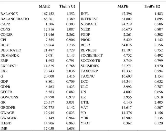
4. Model evaluation
The ability of the model to replicate the endogenous variables is based on an ex post simulation for the period 2005 to 2009. The following two commonly applied statistical measures will be used to evaluate the model:
a) The mean absolute percent error (MAPE) is the average absolute percent error. To arrive at the MAPE one must take the sum of the ratios between the forecast error and the actual realization of the respective variable times 100 (to get the percentage) and divide by the number of forecasting periods. The MAPE is defined by the following formula:
∑ | ̂ | (5)
b) Theil’s inequality coefficient U2. Theil’s inequality coefficient U2 compares the forecast with a naïve no-change forecast. In the case of five-year averages this means that the average of the past five years is taken as the benchmark forecast for the outcome in the following five-year period. The U2 statistic will take the value 1 under the naïve forecasting method. Values less than 1 indicate greater forecasting accuracy
9
than the naïve forecasts, values above 1 indicate the opposite. Theil’s U2 statistic is defined by the following formula:
√∑ (
( ̂ )
)
∑ (
)
(6)
In both equations, x and ̂ denote the actual and the forecast value, respectively, of the variable, t is the time period, and N denotes the number of periods. In the ex post simulation, the number of forecasting periods N was equal to 40 quarters, but for the calculation of the MAPE and of Theil’s inequality coefficient, the quarterly time series had been aggregated to annual data, hence in this case N was equal to 5 years (2005 to 2009).
The results in TABLE 3 in the appendix show that in half of the cases Theil’s inequality coefficient takes values below 1, implying that for these variables the macroeconometric model beats the naive no-change forecast. For the important variables real GDP growth and inflation, Theil’s U2 is only slightly above unity, and for the labour market indicators employment, unemployment and the unemployment rate it is clearly below 1. Nominal values of the GDP expenditure components can be better traced by the model than the respective real variables.
The model contains behavioural equations for the real GDP components (private and public consumption, gross fixed capital formation, exports and imports), as well as for prices (CPI and the GDP deflator). As can be seen from TABLE 3, the price levels can be replicated very well, and better than the real variables. Hence, when calculating the nominal values by multiplying the real values with the deflator, relatively high and low values of Theil’s inequality coefficient are combined, reducing the inequality coefficients of the GDP expenditure components.
Regarding the mean absolute percent error (MAPE), again prices, wages and the labour market indicators exhibit low values. On the other hand, the effective exchange rates and some fiscal variables cannot be tracked so well by the model.
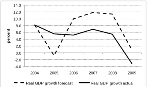
For some important variables, the actual and forecast values are visualised in the figures in the appendix. Overall, the ability of the macroeconometric model for Serbia to replicate the endogenous variables can be regarded as satisfactory, in particular taking the shortness of the available time series into account. The results of the forecast evaluation give reason for optimism regarding the reliability of the model when it is used for forecasting and simulations.
References
Berrer, H., Grozea-Helmenstein D., Weyerstrass K. 2009. A Macroeconomic Model for Serbia. Data, Estimation and Evaluation. Research Report, Economica Institute of Economic Research, Vienna, and Institute for Advanced Studies, Vienna.
Brainard, W.C., Tobin J. 1968. Pitfalls in Financial Model Building. American Economic Review 58(2), 99-122.
Jorgensen, D.W. 1963. Capital Theory and Investment Behavior. American Economic Review, Papers and Proceedings 53.
Keynes, J.M. (1936). The General Theory of Employment, Interest and Money. Macmillan Cambridge University Press.
Weyerstrass, K., Neck, R. (2007), SLOPOL6: A Macroeconometric Model for Slovenia, International Business and Economics Research Journal, Vol. 6, No. 11, 81-94.
Weyerstrass, K., Neck, R., Haber, G. 2001. SLOPOL1: A Macroeconomic Model for Slovenia, International Advances in Economic Research, Vol. 7, No. 1, 20-37.
OECD 2001. Measuring Capital. OECD Manual. Measurement of Capital Stocks, Consumption of Fixed Capital and Capital Services. Paris.
10
OECD 1997. Flows and Stocks of Fixed Capital 1971 – 1996. Paris.
Roberts, B. V. 2002. An analysis of Macedonian economic growth during 1997 – 2001.
Republic of Macedonia, Ministry of Finance, Bulletin 11-12/2002.
Taylor, J.B. 1993. Discretion versus Policy Rules in Practice. Carnegie-Rochester Conference Series on Public Policy, 39, 195-214.
Tobin, J. 1969. A General Equilibrium Approach to Monetary Theory. Journal of Money, Credit, and Banking 1(1), 15-29.
Tobin, J. 1978. Monetary Policies and the Economy: The Transmission Mechanism. Southern Economic Journal 44(3), 421-431.
Appendix
In the following, t-statistics are provided in parentheses below the estimated coefficients. The adjusted R² is the coefficient of determination, adjusted for the degrees of freedom. LM denotes the Breusch-Godfrey test for serial correlation. Unlike the Durbin-Watson statistic for AR(1) errors, the LM test may be used to test for higher order ARMA errors and is applicable whether or not there are lagged dependent variables.
The null hypothesis of the LM test is that there is no serial correlation up to lag order p. The local alternative is ARMA(r,q) errors, where the number of lag terms p = max(r,q). In all equations, p was determined as 2. *, **, *** means that the null hypothesis of no serial correlation has to be rejected at the 10, 5, 1 percent level of significance, respectively.
Model equations Behavioural equations
Consumption of private households
log(CONSR/CONSR-4) = -1.111 + 0.326*log(CONSR/CONSR-4) + 0.721*log(YDR/YDR-4) (1.117) (2.450) (3.647)
- 0.535*log(CONSR-4) + 04185*log(YDR-4) - 0.006*(ILEND-INFL) + 0.094*DUM061-1 (3.775) (2.606) (2.666) (2.468)
R² = 0.712 LM(2) = 1.558
Gross fixed capital formation
log(GFCFR/GFCFR-4)=-1.124 + 0.524*log(GFCFR-1/GFCFR-5) + 0.734*log(GDPR/GDPR-4) (0.671) (6.415) (4.099)
- 0.241*(log(GFCFR-4) + 0.305 *log(DEMANDR-4) - 0.003 ILEND (3.530) (1.678) (3.864) R² = 0.751 LM(2) = 5.623*
Exports of goods and services
log(EXR/EXR-4) = -0.452 + 0.751*log(WTRADE-1/WTRADE-5) (0.402) (3.067)
- 0.107*log(REER/REER-4) - 0.629*log(EXR-4) + 1.071*log(WTRADE-4) (2.557) (7.666) (7.350)
- 0.161*log(REER-4) - 0.857*DUM99 - 0.815*DUM00 - 0.420*DUM021 (3.704) (12.659) (10.432) (3.652)
R² = 0.924 LM(2) = 13.197***
11 Imports of goods and services
log(IMR/IMR-4) = -6.889 + 0.348*log(IMR-1/IMR-5) + 1.721*log(GDPR/GDPR-4) (1.725) (3.149) (3.274)
+ 0.244*log(REER/REER-4) - 0.975*(log(IMR-4) + 1.341*log(GDPR-4) (2.839) (5.098) (3.467)
+ 0.376*log(REER-4) (2.707)
R² = 0.667 LM(2) = 2.447 Employment
log(EMP/EMP-4) = -0.010 + 0.498*log(EMP-1/EMP-5) + 0.134*log(GDPR/GDPR-4) (2.156) (5.938) (2.916)
- 0.043*log(ULC-1/ULC-5) - 0.081*DUM02 (2.672) (6.258)
R² = 0.737 LM(2) = 2.517
Gross wage
log(GWAGE/GWAGE-4) = 3.805 + 0.562*log(CPI/CPI-4) + 0.889*log(PROD/PROD-4) (5.297) (5.661) (4.614)
- 0.021*(UR-NAIRU) - 0.676*(log(GWAGE-4) + 0.811*log(CPI-4)) + 0.305*log(PROD-4) (1.649) (8.038) (6.490) (1.902)
R² = 0.926 LM(2) = 13.799***
Consumer price index
log(CPI/CPI-4) = 0.039 + 0.101*log(OILDIN/OILDIN-4) + 0.302*log(GWAGE/GWAGE-4) (2.446) (5.697) (4.562)
+ 0.598*log(UTIL-2/UTIL-6) + 0524*DUM01 - 0402*DUM014 (3.729) (10.157) (5.781)
R² = 0.928 LM(2) = 8.247* GDP deflator
log(PGDP/PGDP-4) = -0.003 + 0.923*log(PGDP-1/PGDP-5) + 0.085*log(CPI/CPI-4) (0.631) (19.590) (2.116)
+ 0.217*DUM001 - 0.401*DUM021 (10.849) (15.844)
R² = 0.990 LM(2) = 2.211
Short-term interest rate (Taylor rule)
NBSRATE = 0.501*NBSRATE-1 + 0.057*INFL + 0.050*UTIL + 6.777*DUM061 (5.166) (2.367) (4.489) (2.673)
R² = 0.832 LM(2) = 9.524***
12 Long-term interest rate (term structure of interest rates)
ILEND-ILEND-4 = -0.149 + 0.603*(ILEND-1-ILEND-5) + 0.376*(NBSRATE-NBSRATE-4) (0.446) (17.123) (6.782)
- 20.540*DUM014 (9.947)
R² = 0.976 LM(2) = 1.621
Nominal effective exchange rate
log(NEER/NEER-4) = -0.030 + 0.919*log(NEER-1/NEER-5) (1.137) (14.822)
- 1.006*log(DINEUR/DINEUR-4) + 0.927*log(DINEUR-1/DINEUR-5) (16.180) (10.893)
R² = 0.931 LM(2) = 32.998***
Real effective exchange rate
log(REER/REER-4) = 0.010 + 0.844*log(REER-1/REER-5) + 0.654*log(NEER/NEER-4) (0.203) (15.554) (10.304)
- 0.490*log(NEER-1/NEER-5) + 0.369*log(CPI/CPI-4) + 0.802*DUM014 (6.553) (3.184) (5.240)
R² = 0.948 LM(2) = 7.787**
Trend TFP extrapolation
log(TRENDTFP/TRENDTFP-4) = 0.031 + 3.614*AR(1) - 5.436*AR(2) + 4.778*AR(3) (29.741) (31.929) (12.855) (6.591) - 3.610*AR(4) + 3.591*AR(5) - 3.587*AR(6) + 2.258*AR(7) - 0.611*AR(8) (4.242) (4.271) (5.204) (5.906) (6.229) R² = 0.999 LM(2) = 5.814*
NAIRU extrapolation
log(NAIRU/NAIRU-4) = 0.001 + 3.581*AR(1) - 4.901*AR(2) + 2.913*AR(3) (0.067) (27.019) (11.520) (6.404) - 1.334*AR(5) + 1.026*AR(6) - 0.285*AR(7)
(2.860) (2.238) (1.861) R² = 0.999 LM(2) = 2.435
Value added tax (VAT) revenues log(VAT/VAT-4) = -1.698 (2.634)
+ 1.107*log((CONS*VATRATE/100)/(CONS-4*VATRATE-4/100)) (7.360)
- 0.861*(log(CONS-4*VATRATE-4/100))) + 0.221*DUM05 (6.007) (8.714) R² = 0.945 LM(2) = 4.382
13 Social security contributions
log(SOCCONTR/SOCCONTR-4) = -3.503 + 0.597*log(SOCCONTR-1/SOCCONTR-5) (3.154) (7.0400
+ 0.600 log(SOCCONTR-1/SOCCONTR-5) (1.734)
+ 0.165*log((EMP*GWAGE*SOCCONTRATE/100)/(EMP-4*GWAGE-4*SOCCONTRATE-4/100)) (1.734)
- 0.633*(log(SOCCONTR-4) + 0.453*(log(EMP-4*GWAGE-4*SOCCONTRATE-1/100))) (5.261) (4.639)
- 0.247*DUM051 - 0.088*DUM062 - 0.106*DUM071 (6.520) (2.435) (2.928)
R² = 0.905 LM(2) = 5.497* Personal income tax revenues
log(TAXINC/TAXINC-4) = -6.147 + 0.153*DUM07 (4.835) (5.312)
+ 0.951*log((EMP*GWAGE*PINCTRATE/100)/(EMP-4*GWAGE-4*PINCTRATE-4/100)) (2.674)
- 0.520*(log(TAXINC-4) + 0.503*(log(EMP-4*GWAGE-4*PINCTRATE-4/100))) (4.268) (3.561)
R² = 0.737 LM(2) = 2.713 Corporate income tax revenues
log(TAXCORP/TAXCORP-4) = -0.034 + 0.524*log(TAXCORP-2/TAXCORP-6) (0.375) (3.875)
- 0.575*DUM0912 + 1.321*log((GDP-2*CORPTRATE-2)/(GDP-6*CORPTRATE-6)) (5.334) (2.038)
R² = 0.765 LM(2) = 2.621 Remaining government revenues
log(REVREST/REVREST-4) = -0.014 + 1.172*log(GDP/GDP-4) + 0.430*DUM04 (0.342) (4.568) (5.245)
+ 0.345*DUM061 (4.232)
R² = 0.744 LM(2) = 6.357**
Government consumption
log(G/G-4) = 0.058 + 0.196*log(G-1/G-5) - 0.468*log(DEBT-1/DEBT-5) + 0.604*DUM03 (1.766) (2.037) (1.927) (6.324)
R² = 0.715 LM(2) = 21.432***
Government consumption (public finance statistics)
log(GOVCONS/GOVCONS-4) = -0.092 + 0.132*log(GOVCONS-1/GOVCONS-5) (2.292) (2.278)
+ 0.961*log(G/G-4) - 0.451*log(GOVCONS-4/G-4) (4.320) (4.203)
R² = 0.720 LM(2) = 6.184**
14 Social benefits
log(SOCBENEFIT/SOCBENEFIT-4) = 0.038 + 0.517*log(SOCBENEFIT/SOCBENEFIT-4) (1.313) (2.916)
+ 0.282*log(GWAGE/GWAGE-4) (2.195)
R² = 0.508 LM(2) = 0.974 Subsidies
log(SUBSIDIES/SUBSIDIES-4)=-6.692 + 3.844*log(GDP/GDP-4) - 0.590*log(SUBSIDIES-4) (2.660) (4.153) (3.926)
+ 0.909*log(GDP-4) - 0.454*DUM071 - 0.441*DUM072 - 0.512*DUM083 (3.937) (2.477) (2.400) (2.653)
R² = 0.627 LM(2) = 4.043
Interest payments on outstanding public debt
log(INTEREST/INTEREST-4) = -4.558 + 0.756*log(INTEREST-1/INTEREST-5) (2.282) (4.399)
+ 0.836*log(DEBT*ILEND/DEBT-4*ILEND-4) + 0979*DUM081 (2.273) (2.793)
R² = 0.603 LM(2) = 0.494
Remaining government expenditures
log(EXPREST/EXPREST-4)=- 0.765*(log(EXPREST-4)+0.601*log(GDP-4))-1.160*DUM053 (5.977) (6.144) (3.582) R² = 0.627 LM(2) = 2.071
Identities
oildin = oilusd * dinusd gwager = gwage / cpi * 100 infl = (cpi / cpi-4 - 1) * 100
ucc = ilend – ((pgdp / pgdp-4 - 1) * 100) + deprate prod = gdpr / emp
ulc = gwage / prod un = lforce - emp ur = un / lforce * 100
gdpr = consr + gr + gfcfr + inventr + exr - imr grgdpr = (gdpr / gdpr-4 - 1) * 100
gdp = gdpr * pgdp / 100
yd = gdp - taxinc - vat - soccontr + socbenefit ydr = yd / cpi * 100
cons = consr * pgdp / 100 gr = g / pgdp * 100
demandr = consr + gr + gfcfr + inventr + exr
balance = taxinc + taxcorp + vat + soccontr + revrest - socbenefit - subsidies - govcons - interest - exprest
balanceratio = (balance+balance-1+balance-2+balance-3) / (gdp+gdp-1+gdp-2+gdp-3) * 100 debt = debt(-1) - balance + deltadebt
debtratio = debt / (gdp + gdp-1 + gdp-2 + gdp-3) * 100 capr = capr(-1) * (1 - deprate / 100) + gfcfr
trendcapr = trendcapr(-1) * (1 + @pc(capr) / 100)
15 trendemp = lforce * (1 - nairu / 100)
log(ypot) = 0.7 * log(trendemp) + 0.3 * log(trendcapr) + log(trendtfp) util = gdpr / ypot * 100
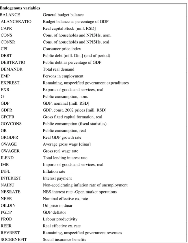
TABLE 1 List of Variables
Endogenous variables
BALANCE General budget balance
ALANCERATIO Budget balance as percentage of GDP CAPR Real capital Stock [mill. RSD]
CONS Cons. of households and NPISHs, nom.
CONSR Cons. of households and NPISHs, real
CPI Consumer price index
DEBT Public debt [mill. Din.] (end of period) DEBTRATIO Public debt as percentage of GDP DEMANDR Total real demand
EMP Persons in employment
EXPREST Remaining, unspecified government expenditures EXR Exports of goods and services, real
G Public consumption, nom.
GDP GDP, nominal [mill. RSD]
GDPR GDP, const. 2002 prices [mill. RSD]
GFCFR Gross fixed capital formation, real GOVCONS Public consumption (fiscal statistics)
GR Public consumption, real
GRGDPR Real GDP growth rate
GWAGE Average gross wage [dinar]
GWAGER Gross real wage rate ILEND Total lending interest rate
IMR Imports of goods and services, real
INFL Inflation rate
INTEREST Interest payment
NAIRU Non-accelerating inflation rate of unemployment NBSRATE NBS interest rate -Open market operations NEER Nominal effective ex. rate
OILDIN Oil price in dinar
PGDP GDP deflator
PROD Labour productivity
REER Real effective ex. rate
REVREST Remaining, unspecified government revenues SOCBENEFIT Social insurance benefits
16 SOCCONTR Social contributions
SUBSIDIES Subsidies
TAXCORP Corporate income tax
TAXINC Personal income tax
TRENDCAPR Trend of capital stock TRENDEMP Trend of employment
TRENDTFP Trend of total factor productivity
UCC User cost of capital
ULC Unit labour costs
UN Unemployed persons
UR Unemployment rate
UTIL Capacity utilisation rate
VAT Value added tax revenues
YD Personal disposable income
YDR Real personal disposable income
YPOT Potential output
Exogenous variables
CORPTRATE Corporate income tax rate
DELTADEBT Diff. between change in debt level and budget balance DEPRATE Quarterly depreciation rate of capital stock (7 % p.a.) DINEUR Exchange Rate Dinar / Euro
DINUSD Exchange Rate Dinar / US Dollar DUM00 Dummy variable, 1 in 2000 DUM001 Dummy variable, 1 in 2000q1 DUM01 Dummy variable, 1 in 2001 DUM014 Dummy variable, 1 in 2001q4 DUM02 Dummy variable, 1 in 2002
DUM021 Dummy variable, 1 in the 1st quarter of 2002 DUM03 Dummy variable, 1 in 2003
DUM041 Dummy variable, 1 in 2004q1 DUM05 Dummy variable, 1 in 2005 DUM051 Dummy variable, 1 in 2005q1 DUM054 Dummy variable, 1 in 2005q4 DUM061 Dummy variable, 1 in 2006q1 DUM062 Dummy variable, 1 in 2006q2 DUM07 Dummy variable, 1 in 2007 DUM071 Dummy variable, 1 in 2007q1 DUM072 Dummy variable, 1 in 2007q2 DUM081 Dummy variable, 1 in 2008q1 DUM083 Dummy variable, 1 in 2008q3
DUM0912 Dummy variable, 1 in 2009q1 and 2009q2