A Case for Incomplete Markets

IHS Economics Series Working Paper 313

June 2015

A Case for Incomplete Markets

Lawrence Blume

Timothy Cogley

David Easley

Thomas Sargent

Viktor Tsyrennikov

Impressum Author(s):

Lawrence Blume, Timothy Cogley, David Easley, Thomas Sargent, Viktor Tsyrennikov Title:

A Case for Incomplete Markets ISSN: Unspecified

2015 Institut für Höhere Studien - Institute for Advanced Studies (IHS) Josefstädter Straße 39, A-1080 Wien

E-Mail: o ce@ihs.ac.atffi Web: ww w .ihs.ac. a t

All IHS Working Papers are available online: http://irihs. ihs. ac.at/view/ihs_series/

This paper is available for download without charge at:

https://irihs.ihs.ac.at/id/eprint/3548/

A Case for Incomplete Markets

Lawrence E. Blume

, Timothy Cogley

, David A. Easley

, Thomas J. Sargent

and Viktor Tsyrennikov

1Cornell University and Institute for Advanced Studies

2New York University

3Cornell University

4New York University and Hoover Institution

5IMF

June 2015

All IHS Working Papers in Economics are available online:

http://irihs.ihs.ac.at/view/ihs_series/ser=5Fwps=5Feco/

Economics Series

Working Paper No. 313

A Case for Incomplete Markets ^∗

Lawrence E. Blume

Timothy Cogley

David A. Easley

Thomas J. Sargent

Viktor Tsyrennikov

June 11, 2015

Abstract

We propose a new welfare criterion that allows us to rank alternative financial market structures in the presence of belief heterogeneity. We analyze economies with complete and incomplete financial markets and/or restricted trading possibilities in the form of borrowing limits or transaction costs. We describe circumstances under which various restrictions on financial markets are desirable according to our welfare criterion.

Keywords: social welfare, heterogeneous beliefs, spurious unanimity, speculation, pessimism, incomplete markets, financial regulation

1 Introduction

A conventional wisdom in the economics profession is that complete markets are good. The welfare theorems state that complete markets outcomes are

∗We would like to thank Jonathan Parker for a helpful and detailed discussion. We would also like to thank V.V. Chari, Vincenzo Quadrini, and participants in the following workshops and seminars: 2014 SITE conference, 2014 ITAM Macroeconomics Workshop, 2013 NBER Summer Institute, 2013 Econometric Society Australian meetings, 2012 North American Econometric Society meetings, 2012 Cornell/PennState Macroeconomics work- shop, and the Joint Vienna Macroeconomics Seminar.

†Cornell University, lHS, lb19@cornell.edu

‡New York University, tc60@nyu.edu

§Cornell University, dae3@cornell.edu

¶New York University and Hoover Institution, ts43@nyu.edu

kIMF, viktor.tsyrennikov@gmail.com

Pareto optimal and that any optimal allocation can be realized by trade in complete markets with an appropriate lump-sum transfer scheme. So putting limits on trade, by foreclosing trading opportunities, leaves potential mutual gains unrealized. This “wisdom” has practical consequences. Arguments for the privatization of social security and against the regulation of financial markets rely in part on the assertion that barriers to trade are bad things.

Complete markets have their critics. Some say that traders have market power and that their exploitation can be limited only by constraining trade.

Others argue that market outcomes, though optimal, are bad in other ways;

since lump-sum transfers are impossible, the sacrifice of dead-weight loss is necessary to achieve other goals. These critiques are empirical. The degree of market power could be large or small. Lump-sum transfers are not so much impossible as they are difficult to execute. Consequently, these concerns are typically considered to be second-order.

We offer here a different and perhaps more fundamental critique. When markets allocate contingent claims among expected-utility-maximizing agents, Pareto optimality with ex ante beliefs is an inappropriate welfare criterion except in the instance where all traders have identical beliefs over states of the world. This critique is detailed in section 3, after an infinite-horizon model of trade in a single consumption good with complete markets is de- veloped in section 2. If the “true distribution of states” were known to an omniscient social planner, Pareto calculations with correct beliefs is an ob- vious fix. Omniscient social planners are rare, however, and without them there is no alternative welfare requirement that obviously ameliorates the issues raised in section 3. We investigate the magnitude of the problem through simulations of competitive equilibria. The simulations of sections 5, 6 and 7 examine several policy alternatives to complete markets in Marko- vian instances of the model of financial restrictions developed in section 4, and explore the size and location of the set of potentially true distributions for which the policies would lead to a true welfare improvement with respect to several distinct welfare criteria. We conclude in section 8 with a discussion of the theoretical and the policy implications of our findings.

2 The model

We assume that time is discrete and begins at date 0. At each date a state is

drawn from the set

=

1, . . . , S

. The set of all sequences of states is Σ with

representative sequence σ = (s

, s

, ...), called a path. Let σ

= (s

, ..., s

) denote the partial history through date t. We use ˜ σ

σ

to indicate that a path ˜ σ coincides with a path σ up through period t.

The set Σ together with its product sigma-field is the measurable space on which everything is built. Let P

denote the “true” probability measure on Σ. For any probability measure P on Σ, P

(σ) is the (marginal) probability of the partial history σ

: P

(σ) = P (

σ

S

S

).

In the next few paragraphs we introduce a number of random variables of the form x

(σ). All such random variables are assumed to be date-t mea- surable; that is, their value depends only on the realization of states through date t. Formally,

is the σ-field of events measurable at date t, and each x

(σ) is assumed to be

-measurable.

An economy contains I consumers, each with consumption set

. A consumption plan c : Σ

t=0R⁺

is a sequence of

-valued functions

c

(σ)

in which each c

is

-measurable. Each consumer is endowed with a particular consumption plan, called the endowment stream. Consumer i’s endowment stream is denoted e

. The aggregate endowment stream is denoted by ¯ e:

¯ e

(σ) =

I

X

i=1

e

(σ).

An allocation is a profile of consumption plans, one for each individual. The allocation (c

, . . . , c

) is feasible if for all σ and t,

i

c

(σ)

e

(σ) = 0.

Consumer i’s preferences on consumption plans are described by a belief or forecast distribution P

, a probability distribution on Σ, a discount factor 0 < β

< 1, and a payoff function u

:

. The utility consumer i assigns to consumption plan c is the expectation of the average discounted value of the sequence of payoff realizations:

U

(c) = (1

β

)E

X

t=0

β

u

(c

(σ))

. (1)

Notice that beliefs are indexed by individual names. Different individuals may believe different things about the future, and these beliefs need not coincide with what will actually happen. The true state process is a stochastic process on

, characterized by a probability distribution P

on Σ, and it may be the case that for no distinct i, j

0 does P

= P

. We will impose some constraints on how different beliefs can be.

We assume the following properties of the payoff function:

A1.

Each u

:

(

,

) is C

, strictly increasing and strictly con- cave.

A2.

Each u

satisfies an Inada condition at 0: lim

u

(c) =

. We assume the following properties of the aggregate endowment:

A 3.

The aggregate endowment is uniformly bounded from above and away from 0:

∞

> F = sup

t,σ

¯

e

(σ)

inf

t,σ

e ¯

(σ) = f > 0.

Finally, we assume that anything is possible at any date, and that indi- viduals believe this to be true:

A 4.

For all individuals i, all dates t and all paths σ, the distributions P

(s

σ

) for i

0 have full support.

We will often refer to agents as being optimistic or pessimistic. We say that a type-i agent is optimistic after history σ

if E

[e

σ

] > E

[e

σ

].

Pessimism is defined analogously.

3 Welfare economics of heterogeneous beliefs

The welfare analysis of market outcomes begins with the Pareto order, taking preferences as given. “Tastes,” say Stigler and Becker [1977, p. 76], “are the unchallengeable axioms of a man’s behavior: he may properly (usefully) be criticized for inefficiency in satisfying his desires, but the desires themselves are data.” Tastes, they say, “are not capable of being changed by persuasion.”

In contingent-claims markets, “Pareto optimality” is taken to be with

respect to ex ante preferences (tastes); that is, ex ante, or time-0, expected

utility. While we do certainly agree that tastes for apples and oranges, work

and leisure, etc., are to be taken as given, we dispute the claim that ex ante

preferences on contingent claims are above dispute. Time-separable expected

utility representations of these preferences have three components: attitudes

towards risk, the rate of time preference, and beliefs about the realization

of states. While risk attitudes and discount factors may be unarguable,

beliefs are not. When market participants have different beliefs, not all can

be right, and those who are wrong are making decisions that they would

regard as incorrect if only they had correct beliefs. Finally, if beliefs were

an indisputable attribute of tastes there would be no role for expectation- managing policies, and the rational expectations hypothesis would never be conceived.

3.1 Spurious unanimity

Ithaca NY, the home of three of us, has a pedestrian mall. It is still ser- viceable, but would benefit from renovation. The work, however, will be costly. Suppose that half the town believes that revitalization will enhance Ithaca’s attraction as a summer tourist destination. This group believes that crowds of tourists will bring more business opportunities and badly needed tax revenues. The other half of the town believes that revitalization will make downtown more pleasant without materially perturbing downtown’s summer population density, thereby enhancing the quality of life. The town is unanimous in its support for the project. Is unanimity of preference a good argument for undertaking the project? Not according to Mongin [2005], who calls this problem “spurious unanimity”. He argues that not only pref- erences themselves, but the reasons why people hold the preferences they have, need to be considered in making welfare claims. This is clear in the mall-renovation case. Suppose that many editorials have appeared in the lo- cal newspaper, many public meetings have been held, and the issue has been thoroughly aired. It is common knowledge, then, that individuals believe different things. It is common knowledge, then, that if the mall is renovated, half the town will be unhappy with the result. It is common knowledge that the renovation cannot be an ex post Pareto improvement. There is disagree- ment only over who is in which half. Suppose there are N different possible states of the world rather than 2, and that the population is divided equally into N groups. Individuals in any group will benefit from a proposal only if “their” state of the world occurs and will be harmed otherwise, and each individual is sure that the state beneficial to him will occur. It is then com- mon knowledge that only fraction 1/N of the population will be made better off, that fraction N

1/N will be made worse off. Imagine that N is large.

The justification of the proposal by ex ante Pareto optimality is not at all

1The assumption of “common knowledge of prior beliefs” is often used, following Au- mann [1976], to justify common beliefs. Common prior arguments are critically discussed in Morris [1995]. To his analysis we add that the entire apparatus of belief about beliefs about beliefs is simply misplaced in models of trade in large anonymous markets, wherein one individual may have no idea of who or what is on the other side of his transaction.

compelling.

The problem of spurious unanimity is even more compelling when ex- pected utility decision makers choose over alternatives with random payoffs.

Imagine now that two decision-makers are choosing between two policies,

and

. Policy

gives outcome a on event E and b on E

. Policy

is the mirror-image; it gives outcome b on E and a on E

. Individuals 1 and 2 each have a payoff function and a prior belief, which are as follows:

Individual 1 u

(a) = 1, u

(b) = 0, ρ

(E) = 0.99, Individual 2 u

(a) = 0, u

(b) = 1, ρ

(E) = 0.01.

Each individual prefers policy

to policy

. Unanimity is a consequence of their divergent beliefs. Given their payoff functions, if they shared a common belief they could never agree on a policy except in the case where they both believe each state is equally likely.

Of course, if one believes that all individuals have common, correct be- liefs then spurious unanimity is not an issue and ex ante Pareto optimality is an appropriate welfare criterion. We do not find this restriction on beliefs compelling. It certainly does not follow from Savage’s (1954) subjective ex- pected utility theorem. It is instead a restriction on preferences which goes far beyond the notion of rationality embedded in Savage. In fact, even the ability to reason about the probabilities in Savage’s representation as beliefs is not as simple as is normally supposed. We discuss this issue in Appendix A.1.

3.2 The ex ante welfare economics of contingent claims

Because beliefs are not above dispute, we are concerned with two Pareto orders. The usual welfare analysis is concerned with the ex ante Pareto order, and because individuals would choose to adopt the true distribution if only they knew it, we are also concerned with the true Pareto order which is the order that obtains when each individual computes expected utility with the true distribution

.

If individuals disagree, then in economies of the type described in Section

2, these two orders differ. That is, ex ante optimal contingent claims for

given beliefs P

, . . . , P

, with P

= P

, for some i and j , cannot be true

Pareto optimal for any P

.

Proposition 1.

If the economy contains two individuals i and j such that for some t and some path σ, P

(σ)

= P

(σ), then no ex ante Pareto optimal allocation in which c

, c

= 0 can be optimal for any true distribution P

. Proof. If P

(σ)

= P

(σ), then there must exist some other path σ

such that P

(σ

)/P

(σ

)

= P

(σ)/P

(σ), else probabilities cannot sum to one. The first-order conditions for optimality on path σ imply that

u

c

(σ)

u

c

(σ) = λ

β

λ

β

P

(σ) P

(σ) ,

where the λ’s, multipliers for the Pareto optimization problem, are both positive as c

, c

= 0. Suppose now that the allocation is true Pareto optimal for some P

. Then first-order conditions imply that there will be positive multipliers γ

and γ

such that

u

c

(σ) u

c

(σ) = γ

γ

β

β

.

Consequently the vectors (γ

β

, γ

β

) and λ

β

P

(σ), λ

β

P

(σ)

are propor- tional.

Now consider path σ

. Since the allocation is truly optimal, it must be the case that:

u

c

(σ

) u

c

(σ

) = γ

γ

β

β

. Since the allocation is also ex ante optimal:

u

c

(σ

)

u

c

(σ

) = λ

β

λ

β

P

(σ

) P

(σ

) .

Thus P

(σ

)/P

(σ

) = P

(σ)/P

(σ), which is a contradiction.

When discount factors are identical, there is in fact a simple necessary condition for true Pareto optimality: Everyone’s consumption is bounded away from 0.

Corollary 1.

If individuals have identical discount factors, if the allocation

c is true-Pareto optimal, and if for all i, c

= 0, then for each individual i

and all σ, lim inf

c

(σ) > 0.

Proof. This follows immediately from the fact that the first order conditions are independent of P

, that the welfare weights are positive, and that aggre- gate endowments are uniformly bounded above and below across paths.

Another necessary condition for true optimality is that there is no spec- ulation on irrelevant states (frivolous uncertainty).

Corollary 2.

Suppose that c is true-Pareto optimal, that c

= 0 for all i, and that the endowment allocation at date t is constant on some event E, that is, for σ, σ

E, e

(σ) = e

(σ

). Then for all individuals c

(σ) = c

(σ

).

Proof. Since the allocation is true-Pareto optimal and c

= 0 for all i, it must be the case that:

u

c

(σ) u

c

(σ) = γ

γ

β

β

= u

c

(σ

)

u

c

(σ

) ,

i, j.

Then e

(σ) = e

(σ

) on E and the fact that the allocation c is feasible imply the desired result.

Proposition 1 and the first welfare theorem suggest that the introduction of some kind of market incompleteness could be welfare-improving, that is, incomplete markets could yield allocations that true-Pareto dominate the complete-markets allocation. Interestingly, someone whose beliefs are correct cannot be ex ante hurt by any true-Pareto improvement. So, as long as majority of the population have correct beliefs, proposals that are true-Pareto improvements should gain political support.

Unfortunately, the mechanism design problem depends critically on the true distribution P

. It is easy to construct examples where there is no allocation that true-Pareto dominates a given ex ante optimal allocation for every possible P

.

Since individuals in the market do not have privileged

2Consider the following example. Two agents with logarithmic preferences believe that the distribution over two possible states is (0.6,0.4) and (0.4,0.6), respectively. Agentiis endowed with 1−e units of consumption good in statei and e units otherwise. In the competitive equilibrium (CE), consumption of agents 1 and 2 are (0.6,0.4) and (0.4,0.6).

The even split is the allocation in which the agents consume 0.5 in each state. It true Pareto dominates the CE allocation only if the true distribution is sufficiently close to (0.5,0.5). If the probability of state 1 under the true distribution exceeds ¯p1≡ln(1.25)/ln(1.5)≈0.55 or is below 1−p¯1, then the even split no longer true-Pareto dominates the CE allocation. In fact, in this case there is no other allocation that true-Pareto dominates the CE allocation for all belief assignments.

knowledge of the true distribution, it would be unreasonable to assume that market designers would have any better knowledge. That is, we want to do distribution-independent market design.

Our solution to this problem is to explore the parameter space. We show that there are market institutions that outperform complete markets over much of the parameter space. “Outperform” here has three meanings.

For the market interventions we consider, through simulation we delineate regions of the model’s parameter space where the intervention is true Pareto superior, where it is better according to a Rawlsian welfare aggregator, and where it is better according to a Bergson-Samuelson social welfare function where the welfare weights are those that solve the ex ante Pareto optimality problem.

3.3 Spurious unanimity: other approaches

Others have addressed the problem of spurious unanimity in contingent claims allocations. Brunnermeier et al. [forthcoming] introduce belief-neutral Pareto optimality. They identify a set of “reasonable beliefs”, potential true distributions, which is the convex hull of the set of individuals’ beliefs. Al- location x is then belief-neutral Pareto superior to allocation y if x is true Pareto superior to y for every true distribution in the set of reasonable beliefs.

The intersection of a collection of Pareto orders is, generally speaking, incred- ibly incomplete. Brunnermeier et al. [forthcoming] reduce incompleteness by examining partial orders induced by Bergson-Samuelson social welfare func- tions, taking weighted averages of each profile of true expected utilities.

Gilboa et al. [2014] offer a somewhat complicated alternative. Allocation x no-bet Pareto improves upon y if x ex ante Pareto improves upon y and if there exists a potentially true probability distribution such that each indi- vidual whose position is ex ante improved in the move from y to x also truly prefers x to y. This is a direct attempt to remove from Paretian calculations the speculative component to trade that is introduced when beliefs disagree.

The no-bet Pareto relation, while acyclic, can be intransitive.

These two proposals delineate the trade offs that arise when considering

potential true distributions. Requiring Pareto improvement with respect to a

large class of potential true distributions for all welfare comparisons thickens

the contract curve; few welfare comparisons can be made. Relaxing this

ordinal uniformity condition, however, and allowing different distributions

for different comparisons, will, generally speaking, introduce intransitivities.

Duffie [2014] also addresses the issue of trading generated by heteroge- neous beliefs and appropriate policy responses to it. He raises issues of how to evaluate welfare in this context and considers the tradeoffs between reducing speculation and trading to hedge risk, provide liquidity or use information.

We do not see any particularly compelling way to undertake welfare anal- ysis when beliefs are heterogeneous. This includes ex ante Pareto optimality.

So in this paper we carry out the more limited task of identifying sets of beliefs and potentially true distributions for which given market restrictions are in some sense welfare-improving in some simple examples. We believe that if, in a carefully calibrated model of economic activity, for some market restriction the set of potentially true distributions for which it is a welfare improvement is large, then there is a strong prima facie case for introducing it.

4 Financial markets, competitive equilibria

In this section, we describe optimization problems of an agent under different financial market designs.

4.1 The complete markets economy

The first and the key market design is (dynamically) complete financial mar- kets. Let Q

(σ) be the date-t price of an Arrow security that pays along path σ. The number of Arrow securities purchased by a type-i agent in period t along history σ is denoted by a

(σ). Then a type-i agent faces the following budget constraint at each date t

c

(σ) +

σ|σ˜ ^t

Q

(˜ σ)a

(˜ σ) = a

(σ) + e

(σ). (2a) Purchases of Arrow securities are subject to natural borrowing limits at each date t

a

(σ)

N

(σ), (2b) constructed as follows. Define the j-period ahead price Q

(σ) = Π

Q

(σ).

Then a natural borrowing limit equals the date-t value of the continuation

of an agent’s endowment plan:

N

(σ) =

∞

X

j=0

X

˜σ|σ^t

Q

(˜ σ)e

(˜ σ). (3) Natural borrowing limits never bind in a competitive equilibrium if a period utility function satisfies our Inada condition (A2). A type-i agent chooses consumption and asset trading plans to maximize life-time utility (1) subject to constraints (2a) and (2b).

We define prices of two assets to which we refer later. The price of a risk-free bond at date t is

q

(σ) =

σ|σ˜ ^t

Q

(˜ σ). (4a)

The price at date t on path σ of a claim to the aggregate endowment is:

q

(σ) =

∞

X

j=0

X

˜σ|σ^t

Q

(˜ σ)e

(˜ σ). (4b)

Definition. The complete financial markets (CM) design is a set of S finan- cial markets where market j trades an Arrow security that pays one unit of consumption good next period if state j realizes. Trading is subject to natural borrowing limits defined above.

Definition. An agent is said to survive if his consumption remains strictly positive forever almost surely-P

.

In addition to standard complete markets, we analyze several other de- signs: complete markets with borrowing limits (CMB), complete markets in which transactions are taxed (CMT), and markets trading only a risk-free bond subject to a borrowing limit (B). We think of these intermediate de- signs as partially regulated financial markets and aim to shed light on the relative desirability of different restrictions.

4.2 A bond economy

Definition. A bond-only financial market design (B) consists of a single mar-

ket that trades a risk-free bond subject to an exogenous borrowing limit.

In the bond economy, a type-i agent faces the following constraints:

c

(σ) + q

(σ)b

(σ) = b

(σ) + e

(σ), (5a) b

(σ)

B

(σ), (5b) where q

(σ) denotes the date-t price of a risk free bond, b

(σ) represents the date-t bond purchases of agent i, and B

(σ) is an exogenous borrowing limit. These borrowing limits have to be sufficiently tight to make sure that all loans are repaid with certainty. Borrowing limits must be tighter than the worst-case date-t value of the continuation of an agent-i’s endowment plan:

˜

inf

σ|σ^t

"

e

(˜ σ) +

∞

X

j=0

Π

q

(˜ σ)e

(˜ σ)

#

.

The above borrowing limit is the largest limit that can (potentially) be im- posed after history σ

on a type-i agent in the bond-only economy. However, unlike in the complete markets economy, an endogenous borrowing limit can- not be determined before solving for a competitive equilibrium. Hence, an exogenous borrowing limit must be imposed instead.

4.3 Borrowing limits

Definition. The complete financial markets with a borrowing limit (CMB) design is a set of S financial markets where market j trades an Arrow security that pays one unit of consumption good next period if state j realizes and zero otherwise. Trading is subject to an exogenous borrowing limit.

Under the complete markets with a borrowing limit design trading is subject to an exogenous borrowing limit B that is tighter than the natural borrowing limits in (2b)

a

(σ)

B. (6)

The financial markets are complete in the sense that a full set of Arrow

securities is traded. Yet, when a tight borrowing limit is imposed, insurance

possibilities are restricted. Speculation opportunities are also limited, which

tames the survival forces analyzed by Blume and Easley [2006] that otherwise

would drive the consumption of agents with less accurate beliefs to zero

asymptotically.

4.4 Transaction costs

Definition. The complete financial markets with a transaction cost (CMT) design is a set of S financial markets where market j trades an Arrow security that pays one unit of consumption good next period if state j realizes and zero otherwise. Trading is subject to a transaction cost.

Under this design the budget constraint (2a) is replaced with the following c

(σ) +

σ|σ˜ ^t

Q

(˜ σ)a

(˜ σ) + τ

˜σ|σ^t

[a

(˜ σ)

a

(σ)]

= a

(σ) + e

(σ) + T

(σ)/2, (7) where T

(σ) is the total transaction tax revenue. Our transaction tax design embeds two important assumptions. First, the transaction tax is assumed to be a quadratic function of security purchases to insure continuity of demands for securities. Second, we rebate the transaction tax back to investors as equal lump sums.

A transaction cost limits speculation opportunities, as does a borrowing limit, but agents are not guaranteed to survive. The two alternatives differ in how they control potential welfare losses: a transaction cost slows the rate at which agents can lose wealth, and a borrowing limit imposes a bound on how much wealth can be lost.

5 Welfare criteria

We require some welfare criterion in order to discuss the welfare consequences of market restrictions. Although we do not want to commit to a particular criterion, any acceptable criterion should satisfy some obvious desiderata.

First, as we have argued, it cannot be based on individual welfare computed

ex ante. We consider individuals who chose optimally, given their preferences,

but we evaluate their welfare using the true probability on states. Second, we

do not want to evaluate social welfare using any particular truth as we see no

justification for assuming that the social planner, who we view as choosing

market restrictions, knows the truth when individuals do not know it. So, we

evaluate welfare over a set of possible truths. Third, we do not want to design

market restrictions that work only for particular configurations of individual

beliefs. Once we drop the usual restriction that beliefs are correct, we see

no justification for placing joint restrictions on, possibly incorrect, beliefs of individuals. Therefore we evaluate welfare over a set of individual beliefs.

Finally, for any given individual beliefs and truth, we need to aggregate individual payoffs. Here too we see no compelling argument for any partic- ular aggregator and we instead consider several possibilities: one based on a Rawlsian criterion as well as one based on a Bergson-Samuelson criterion.

We admit at the outset that this approach requires that we take utility to be interpersonally comparable. The burgeoning literature on ex ante optimality with heterogeneous beliefs has yet to produce a satisfactory ordinal way of proceeding; so at the present time social welfare functions are the only way to go forward. Definition. A utility aggregator

: R

R is a non-decreasing continuous function such that

(U )

[min

U

, max

U

],

U

R

.

The Pareto welfare criterion uses:

W

(U

, .., U

) =

I

X

i=1

θ

U

(8)

for some exogenously given vector of Pareto weights θ

∆

. Another possi- bility is the Rawlsian utility aggregator:

W

(U ) = min

i

U

. (9)

Definition. Let

be a set of admissible beliefs and let

= (P

, ..., P

)

denote a belief assignment. Let P

be a data generating process, where

is a set of admissible data generating processes. Let c(

) be a competitive equilibrium allocation under a financial market structure

and a belief assignment

. Then the social welfare function using a utility aggregator

is:

P

min

min

P∈B^IW

U

(c

(

))

. (10)

This welfare criterion emerges from three analytic choices. The first choice

is that of

. Fix the beliefs assignment

= (P

, ..., P

) and the true data

generating process P

. By choosing a market structure

the designer

effectively selects an allocation (c

(

), ..., c

(

)) and the associated

distribution of utilities (U

, ..., U

). A utility aggregator

transforms

the distribution of utilities into a social welfare measure. A designer using (9) would choose a financial market structure that benefits the least-advantaged members of society. That is the designer would adhere to one of the principles of justice proposed in Rawls [1971].

A designer using (8) would act similarly to a Pareto planner. But the utility aggregator (8) presents a new degree of arbitrariness: What weights should a designer use? One could choose θ

= 1/I,

i, the choice that is attractive in ex-ante symmetric environments. One could also choose θ to be a vector of “market weights”.

These two choices are special cases of Bergson-Samuelson social welfare functions. However, any set of weights is arbitrary. The paternalistic designer using the Rawlsian aggregator (9) is spared the obligation of deciding a fair set of weights.

The second choice is the minimization over belief assignments. Our moti- vation is that in reality many configurations of beliefs are possible. Each such configuration may support a different financial market design. For example, some agents may be optimistic and undertake excessively risky investments that could drive them quickly out of financial markets. Imposing borrowing limits may be desirable in this case. On the other hand, pessimistic agents might over-invest in safe assets. They would still be driven out of finan- cial markets, but perhaps at a slower rate. Financial regulation in this case would have to strike a balance between saving agents from financial ruin and encouraging diversification. A rational planner would need to take into account any available information on the distribution of beliefs in the popu- lation. We minimize over beliefs for two reasons. First, our goal in this paper is to provide examples of how complete markets can go astray, and comput- ing worst cases satisfies that need. Second, one can view minimization over

3Rawls [1971] argues that a fair social choice can only be made in a hypothetical

“original position”:

No one knows his place in society, his class position or social status, nor does anyone know his fortune in the distribution of natural assets and abilities, his intelligence, strength, and the like. I shall even assume that the parties do not know their conceptions of the good or their special psychological propensities. The principles of justice are chosen behind a veil of ignorance.

For our purposes, replace “principles of justice” with “design of financial markets.” The veil of ignorance advocated by Rawls allows devising a set of rules that are independent of the current economic fundamentals – beliefs assignment, true data generating process, and wealth distribution.

4This is a vector of weights for which the Pareto and the competitive allocations coincide under Pⁱ =P⁰,∀i. See section 7 for more details.

belief assignments as a Rawlsian approach to social welfare in which each belief assignment corresponds to a different feasible configuration of society and the planner has no ex ante information about the beliefs held by the traders.

6 Examples

We now present the leading example that we use to illustrate economic forces that operate in economies with heterogeneous beliefs. We apply our welfare criterion to compare complete markets with various incomplete market set- tings. In this section, we investigate social welfare using the Rawlsian utility aggregator (9). In section 7, we consider the Pareto criterion using market weights. The two criteria lead to remarkably similar results.

In our economy agents share a common utility function u(c) = c

/(1

γ),

where γ = 2.

There are two types of agents and three states: σ

0, 1, 2

. The economy begins in state 0 and then exits to states 1 and 2.

Endowments are

(e

(σ), e

(σ)) =







(0.5, 0.5) if σ

= 0 (e

, e

) if σ

= 1 (e

, e

) if σ

= 2

,

t, σ. (11)

We assume that e

> e

. Although there is no aggregate uncertainty, indi- viduals face idiosyncratic risk.

Beliefs are specified as follows:

Π

=





0 0.5 0.5 0 p

1

p

0 p

1

p





, (12)

5Other approaches are possible. Phelan and Rustichini [2015], in a different context, take an alternative approach in which each individual (for us each individual defined by some beliefs) is treated a separate person and Pareto optimality takes each of these

“people” directly into account.

6Robustness of our results to the specification of preferences is considered in Appendix A.3.

7The only purpose of the transitory state 0 is symmetry. It insures that agents begin with identical endowments and can trade prior to the first realization of states 1 and 2.

where Π

denotes the true probability transition matrix. Subjective probabil- ities over histories P

(σ) are computed using individual transition matrices.

6.1 Complete markets economy

First, we describe a competitive equilibrium in the complete markets economy when beliefs are homogeneous, but not necessarily correct. Because there is no aggregate uncertainty and preferences are homothetic, both agents con- sume a constant amount. The competitive equilibrium allocation is:

(c

(σ), c

(σ)) = (0.5 + β

(µ

0.5), 0.5

β

(µ

0.5)),

t, σ, (13) where µ

pe

+ (1

p)e

is the expected endowment evaluated using the common beliefs, p. An agent achieves a constant consumption plan by buying an amount A

0.5

e

+ β(µ

0.5) of Arrow securities paying in the state where its income is e

. The quantity of Arrow securities traded in equilibrium,

A

, is small relative to the natural borrowing limit: N

(σ) = e

(σ) + βµ

/(1

β).

Second, we describe a competitive equilibrium with complete markets and heterogeneous beliefs. Suppose that p

= p

and p

= p

. In this case, not only do agents not consume constant amounts, but as shown by Blume and Easley [2006], consumption of a type-2 agent converges to zero:

lim sup

t→∞

c

(σ) = 0 P

a.s. (14)

Following Blume and Easley [2006], we say that type-2 agents do not survive.

The eventual immiseration of agents with incorrect beliefs when market are complete is the source of an instinct that market restrictions could be useful.

Agents invest in Arrow securities for two reasons: income hedging and disagreement. Suppose p

> p

= p

. To hedge income fluctuations, a type-2

8The beliefs on sample paths induced by this structure do not involve learning. Our individuals believe that the exogenous states follow an iid process and each personiis cer- tain aboutpⁱ. The analysis can be extended to include learning. Our general results carry over to this extension as can be seen from the analysis in Blume and Easley [2006]. Com- puting equilibria is, however, much more difficult. Learning in which individuals’ beliefs converge to the true data generating process makes complete markets more attractive, but it does not eliminate the desirability of restrictions on financial markets. Individuals care about the entire process, not just the limit, and so what matters is the speed of learning versus the rate at which the future is discounted.

0.0 0.2 0.4 0.6 0.8 1.0

0 10 20 30 40 50 60 70 80 90 100 period, t

A. Consumption of type-2 individual

-10.0 -5.0 0.0 5.0 10.0

0 10 20 30 40 50 60 70 80 90 100 period, t

B. Financial wealth of type-2 individual

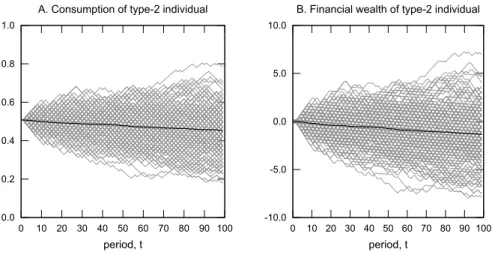
Figure 1: Sample paths of consumption and financial wealth of a type-2 agent in the complete markets economy.

Parameters: β = 0.96, e

= 1/3, e

= 2/3, p

= p

= 0.5, p

= 0.55.

agent buys Arrow securities that pay in state 1 (when his income is low) and sells Arrow securities that pay in state 2 (when his income high). Because a type-2 agent overestimates the probability of state 1, he buys extra securities that pay in this state. So he over-invests in securities that pay in state 1 and under-invests in securities that pay in state 2. These additional trades are “speculative.”

As a result of these trades, a type-2 agent’s consumption increases every time state 1 realizes. The opposite happens if state 2 realizes.

State 1 is less likely than a type-2 agent anticipates. So his investments pay off less than he expects, he loses wealth on average, and his consumption converges to zero.

Figure 1 plots 200 sample paths of consumption (panel A) and financial wealth (panel B) of a type-2 agent for a simple example of the complete markets economy. The solid line in each panel denotes the average across sample paths. Both consumption and wealth drift towards their respective lower bounds. The speed of convergence is slow: for example, after 100 periods a type-2 agent’s consumption decreases from 0.493 to 0.432 along the average path. The decline in financial wealth is more substantial, falling from 0 to -1.524 (or roughly three average individual annual incomes) along

9Speculation is trading activity that is motivated by differences in beliefs and would be absent had all agents had the same beliefs.

0.0 0.2 0.4 0.6 0.8 1.0

0 10 20 30 40 50 60 70 80 90 100 period, t

A. Consumption of type-2 individual Perception Reality

-10.0 -5.0 0.0 5.0 10.0

0 10 20 30 40 50 60 70 80 90 100 period, t

B. Financial wealth of type-2 individual Perception Reality

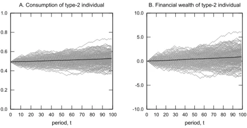
Figure 2: Actual vs perceived sample paths of consumption and financial wealth of a type-2 agent in the complete markets economy.

Parameters: β = 0.96, e

= 1/3, e

= 2/3, p

= p

= 0.5, p

= 0.55.

the average path.

Despite a decline in his consumption and financial wealth, a type-2 agent believes that what happens to him is simply bad luck. Figure 2 demonstrates the difference between actual and perceived outcomes. This figure plots expected, from a point of view of type-2 agent, evolution of his consumption and financial wealth in periods 51-100 assuming that during periods 0-50 he followed the “average path.” Not surprisingly, he expects to prosper. This is a manifestation of another result in Blume and Easley [2006] which applied to our example shows that agent 2 believes that his consumption will converge almost surely to the entire aggregate endowment:

lim sup

t→∞

c

(σ) = 1 P

a.s.

Finally, we present welfare levels for the two types of agents in our ex- ample. As a benchmark, we compute welfare in the complete markets econ- omy when beliefs are homogeneous and coincide with the truth. Assuming p

= 0.50, this benchmark level of welfare, denoted by W

, is

2 for each type. Subjective welfare levels in the heterogeneous beliefs economy are

−

1.943 and

2.124, respectively, for type-1 and type-2 agents. A type-1

agent, whose beliefs coincide with the truth, expects higher welfare than

W

. He is better off in the economy with diverse beliefs as his “speculative”

financial trades allow him to accumulate wealth. A type-2 agent expects welfare level that is lower than W

. This happens because the type-2 agent believes that his endowment stream has a relatively low value. Objective welfare levels (expected utility of equilibrium consumptions computed using the truth) are

1.947 and

2.129, respectively for a type-1 and type-2 agent.

In this example, belief diversity has a substantial impact on welfare: rela- tive to the common beliefs benchmark, a reduction in a type-2 agent’s welfare is equivalent to a permanent 6.45% decline in his consumption.

So welfare of a type-2 agent is low, and hence according to the Rawlsian aggregator, social welfare is low. Two sources contribute to this outcome: consumption volatility and a downward trend in a type-2 agent’s consumption. To quan- tify the contribution of each source, we note that the welfare of a type-2 agent computed along the “average path” is

2.091. Thus, low welfare of a type-2 agent is caused largely by a diminishing trend in his consumption rather than by increased consumption volatility.

6.2 Bond economy

In the bond-only economy, agents can save or borrow by buying or selling bonds, but they cannot transfer income across states. To insure that an equilibrium exists, we impose a borrowing limit as explained in section 4.2.

Since it is impossible to devise a priori a borrowing limit that would never bind, we impose an exogenous, yet generous, limit of 16 average individual annual incomes: B

(σ) = 8,

t, σ.

Continuing with the example from the previous section, we simulate equi- librium consumption and wealth dynamics in the bond economy. As shown in figure 3, consumption and financial wealth for the type-2 agent now grow on average. Consumption increases from an average of 0.492 to 0.526 (panel

10Costs of aggregate fluctuations in a standard RBC model are typically found to be below 0.1%.

11It is natural to ask what would happen in this economy if a type-2 agent were opti- mistic. To answer this we studied the case withp⁰=p¹= 0.50, p²= 0.45. Welfare levels in this case are: U_P¹⁰ =U_P¹¹ =−2.002, U_P²⁰ =−2.063 and U_P²² =−2.058. Here a type-2 agent still has the lower welfare in the economy, but it is not as low. This happens largely because optimism increases the value of his endowment plan. So his consumption while decreasing on average starts from a value above 0.5. If we replaced his consumption plan with an average plan his welfare would be−2.024. So here the welfare loss is attributed mainly to increased consumption volatility. See also section A.2.1.

0.0 0.2 0.4 0.6 0.8 1.0

0 10 20 30 40 50 60 70 80 90 100 period, t

A. Consumption of type-2 individual

-10.0 -5.0 0.0 5.0 10.0

0 10 20 30 40 50 60 70 80 90 100 period, t

B. Financial wealth of type-2 individual

Figure 3: Sample paths of consumption and financial wealth of a type-2 agent in the bond economy.

Parameters: β = 0.96, e

= 1/3, e

= 2/3, p

= p

= 0.5, p

= 0.55, B = 8.

A), and financial wealth rises from an average of 0 to 0.878, or 1.76 average individual annual incomes (panel B). As explained in Cogley et al. [2014], this occurs because the type-2 agent is pessimistic and buys bonds as a pre- cautionary store of value.

Subjective welfare levels are

2.004 and

2.011, respectively, for the type-1 and type-2 agents. So both agents expect to be worse off than in the complete markets economy in which agents have common, correct beliefs.

Objective welfare levels show that despite accumulating financial wealth, a type-2 agent has lower welfare. This occurs because pessimism motivates a type-2 agent to postpone consumption far into the future, which lowers expected utility.

6.3 Bond-only vs complete markets

If (p

= p

= 0.5, p

= 0.55) were the only admissible beliefs, our welfare

criterion (with the Rawlsian aggregator) would select the bond-only design

over the complete markets design. The former awards a substantial welfare

level to both types because it limits speculation while still allowing resources

to be transferred across periods. Under complete markets, type-1 agents

take advantage of the poor forecasting abilities of type-2 agents, eventually

driving them to destitution.

Matters are more complicated when we consider a larger set of admissible beliefs. For instance, suppose (p

, p

)

[0.45, 0.55]

, and p

= 0.5.

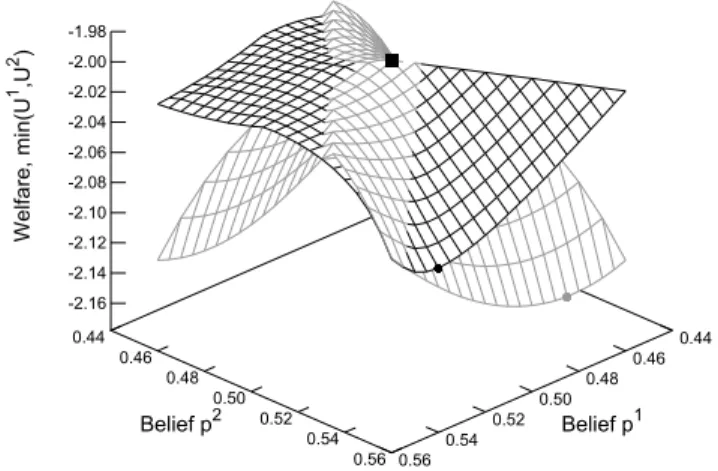
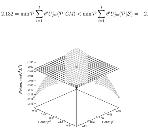
Figure 4 plots the welfare surface min

[U

(c

(p

, p

))] for this belief set.

The lowest welfare level under the bond-only design is

2.011, and it is achieved at (p

, p

) = (0.45, 0.45) and (0.55, 0.55). At these “critical points” (depicted by black points in the figure), beliefs are homogeneous but wrong.

0.46 0.44 0.50 0.48 0.54 0.52 0.56

Belief p¹ 0.44

0.46 0.48 0.50 0.52

0.54 0.56 Belief p²

-2.16 -2.14 -2.12 -2.10 -2.08 -2.06 -2.04 -2.02 -2.00 -1.98

Welfare, min(U1 ,U2 )

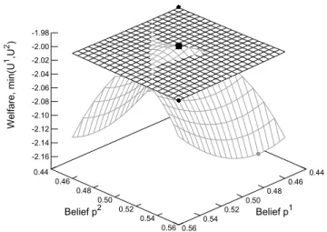
Figure 4: Welfare in example 1: the bond-only (black) vs the complete markets (gray) design. Square point denotes the unconstrained maximum:

(p

, p

, W

) = (0.5, 0.5,

2). Circle points denote belief assignments that attain the lowest welfare under the corresponding design.

Parameters: β = 0.96, e

= 1/3, e

= 2/3, p

= 0.5, B = 8.

The lowest welfare in the complete markets economy is

2.139, and it is achieved at (p

, p

) = (0.45, 0.525) and (0.475, 0.55) (portrayed by gray points in the figure). At the critical points, beliefs are nearly maximally different.

Consider the belief assignment (p

, p

) = (0.45, 0.525). With these beliefs the

12Note that for now, we consider only one possible true data generating process. In section 8, we relax this restriction.

13The shape of this welfare surface is explained in Appendix A.2.

type-1 agent has lower welfare. Two forces act against him. First, his beliefs are less accurate, so his consumption is eventually driven to zero. Second, he is more pessimistic than a type-2 agent, and his endowment stream is valued less – he is subject to a negative wealth effect. But a type-2 agent is also pessimistic, and this activates a wealth effect that reduces a type-2 agent’s welfare.

In this example, our welfare criterion (using the Rawlsian aggregator) selects the bond-only design over the complete markets design because:

−

2.011 = min

P¹,P²

min

i

U

(c

(

B )) > min

P¹,P²

min

i

U

(c

(

CM)) =

2.139.

The complete markets design would be preferred if the set of admissible beliefs were concentrated tightly enough about the truth, for example, if it were reduced to [0.49, 0.51]

.

This is not surprising as the complete markets design is, of course, pre- ferred to the bond-only design with common, correct beliefs. It is surprising, though, that the bond-only design performs so robustly, at least when there is no aggregate risk.

Before we continue with our next market design we would like to describe

the choice made by a designer who is guided by the true-Pareto welfare crite-

rion. Figure 5 plots the set of beliefs for which the bond-only market design

true-Pareto dominates complete markets. The dark gray area denotes belief

assignments for which the bond-only CE allocation true-Pareto dominates the

complete markets CE allocation. Naturally, this occurs where disagreement

is strongest. As explained above, restricting financial trade to risk-free bonds

effectively shuts down speculation, thereby increasing everyone’s utility. The

portion of the region at the bottom right corner is larger than at the top left

corner. This is because these beliefs make agents optimistic and more willing

to speculate. Hence, in our example, regulation is desirable over a larger set

of parameters when agents are optimistic. The light gray area denotes belief

assignments under which the two market designs cannot be ranked because

one agent gains while another loses. It is useful to emphasize that this area is

more than 50% of the whole set of beliefs. It shrinks dramatically when the

truth is varied. The white area denotes belief assignments under which the

complete markets dominate the bond-only design. This area includes beliefs

that coincide with or are close to the truth. It also includes a narrow area

parallel to the “agreement diagonal.” In this portion of the parameter space,

the effect of disagreement is offset by the bias in beliefs towards one of the