A Hierarchical Procedure for the Combination of Forecasts: This is a revised version of Working Paper 228, Economics Series, October 2008, which includes some changes.

IHS Economics Series Working Paper 240

June

2009

A Hierarchical Procedure for the Combination of Forecasts: This is a revised version of Working Paper 228, Economics Series, October 2008, which includes some changes.

The most important change regards the reference of Kisinbay (2007), which was not reported in the previous version. The hierarchical procedure proposed in the paper is based on the approach of Kisinbay (2007), but some modifications of that approach are provided.

Mauro Costantini

Carmine Pappalardo

Impressum Author(s):

Mauro Costantini, Carmine Pappalardo Title:

A Hierarchical Procedure for the Combination of Forecasts: This is a revised version of Working Paper 228, Economics Series, October 2008, which includes some changes.

The most important change regards the reference of Kisinbay (2007), which was not reported in the previous version. The hierarchical procedure proposed in the paper is based on the approach of Kisinbay (2007), but some modifications of that approach are provided.

ISSN: Unspecified

2009 Institut für Höhere Studien - Institute for Advanced Studies (IHS) Josefstädter Straße 39, A-1080 Wien

E-Mail: o ce@ihs.ac.atffi Web: ww w .ihs.ac. a t

All IHS Working Papers are available online: http://irihs. ihs. ac.at/view/ihs_series/

This paper is available for download without charge at:

https://irihs.ihs.ac.at/id/eprint/1923/

"This is a revised version of Working Paper 228, Economics Series, October 2008, which includes some changes. The most important change regards the reference of Kisinbay (2007), which was not reported in the previous version.

The hierarchical procedure proposed in the paper is based on the approach of Kisinbay (2007), but some modifications of that approach are provided."

A Hierarchical Procedure for the Combination of Forecasts*)

Mauro Costantini, Carmine Pappalardo

240

Reihe Ökonomie

Economics Series

240 Reihe Ökonomie Economics Series

A Hierarchical Procedure for the Combination of

Forecasts

Mauro Costantini, Carmine Pappalardo June 2009

Institut für Höhere Studien (IHS), Wien

Institute for Advanced Studies, Vienna

Contact:

Mauro Costantini

Department of Economics University of Vienna BWZ Bruenner Str. 72 1210 Vienna, Austria

: +43/1/4277-37478 fax: +43/1/4277-37498

email: mauro.costantini@univie.ac.at Carmine Pappalardo

ISAE, Institute for Studies and Economic Analysis Rome

Founded in 1963 by two prominent Austrians living in exile – the sociologist Paul F. Lazarsfeld and the economist Oskar Morgenstern – with the financial support from the Ford Foundation, the Austrian Federal Ministry of Education and the City of Vienna, the Institute for Advanced Studies (IHS) is the first institution for postgraduate education and research in economics and the social sciences in Austria. The Economics Series presents research done at the Department of Economics and Finance and aims to share ―work in progress‖ in a timely way before formal publication. As usual, authors bear full responsibility for the content of their contributions.

Das Institut für Höhere Studien (IHS) wurde im Jahr 1963 von zwei prominenten Exilösterreichern – dem Soziologen Paul F. Lazarsfeld und dem Ökonomen Oskar Morgenstern – mit Hilfe der Ford- Stiftung, des Österreichischen Bundesministeriums für Unterricht und der Stadt Wien gegründet und ist somit die erste nachuniversitäre Lehr- und Forschungsstätte für die Sozial- und Wirtschafts- wissenschaften in Österreich. Die Reihe Ökonomie bietet Einblick in die Forschungsarbeit der Abteilung für Ökonomie und Finanzwirtschaft und verfolgt das Ziel, abteilungsinterne Diskussionsbeiträge einer breiteren fachinternen Öffentlichkeit zugänglich zu machen. Die inhaltliche Verantwortung für die veröffentlichten Beiträge liegt bei den Autoren und Autorinnen.

Abstract

This paper proposes a strategy to increase the efficiency of forecast combination. Given the availability of a wide range of forecasts for the same variable of interest, our goal is to apply combining methods to a restricted set of models. To this aim, a hierarchical procedure based on an encompassing test is developed. Firstly, forecasting models are ranked according to a measure of predictive accuracy (RMSFE). The models are then selected for combination such that each forecast is not encompassed by any of the competing forecasts. Thus, the procedure aims to unit model selection and model averaging methods. The robustness of the procedure is investigated in terms of the relative RMSFE using ISAE (Institute for Studies and Economic Analyses) short-term forecasting models for monthly industrial production in Italy.

Keywords

Combining Forecasts; Econometric Models; Evaluating Forecasts; Models Selection, Time series

JEL Classification

C32, C53

Comments

The first draft of this paper was mostly prepared while Mauro Costantini was working as a post- doctorate researcher at ISAE. The authors would like to thank Michael P. Clements and Robert Kunst for their very useful suggestions. The authors would also like to thank the partecipants at the 28th annual International Symposium on Forecasting, Nice 2008. None of them is responsible for any remaining errors. The opinions expressed in this paper are solely the responsibility of the authors and should not be interpreted as reflecting the views of ISAE or its staff.

Contents

1 Introduction 1

2 Forecast encompassing and RMSFE 2

3 Forecast encompassing and combining methods 3

4 Forecasting models 5

5 Empirical results 7

6 Conclusions 9

References 9

Figure and Tables 11

1 Introduction

Forecast combination is often used to improve forecast accuracy. A linear combi- nation of two or more predictions may often yield more accurate forecasts than using a single prediction to the extent that the component forecasts contain useful and independent information (Newbold and Harvey, 2002). To generate independent forecasts two alternative methods can be followed. One is to ex- amine different data, and the other is to use different forecasting methods. On the one hand, the use of several sources of data can add useful information and can also adjust for biases. On the other hand, forecasting combining methods can reduce errors arising from faulty assumption, bias, or mistake data.

This paper considers a hierarchical procedure to increase the efficiency of fore- casting combining methods is provided. The procedure is based on the approach proposed by Kisinbay (2007), but in this paper paper the RMSFE encompassing testing approach is discussed to show under which conditions the encompassing test developed by Harvey, Leybourne and Newbold (1998, hereafter HLN) can be used to check for forecast encompassing in one direction, and a multiple en- compassing test (Harvey and Newbold, 2000) is used to assess the robustness of the model selection strategy.

The procedure consists of several steps. Firstly, the overall forecasts are ranked using RMSFE measure. The forecasting models are then selected for combina- tion using the HLN encompassing test. Thus, the hierarchical approach aims to unit model selection and model averaging methods. Larger weights are assigned to the models with higher forecasting performance and which add information not covered by other models. Estimated forecasts with lower accuracy and that are encompassed by all the other models are discarded as their weights will be insignificant (Hendry and Clements, 2004). For these reasons, the hi- erarchical procedure can be considered as an alternative to the optimal com- bination method based on the variance-covariance matrix of forecasting errors.

The hierarchical algorithm is aimed at selecting a given modelM1with greater forecasting accuracyvis a visthe rivalM2only if the former presents a greater informative content. In general terms, if a given model has a lower RMSFE than the other forecasting models, the sufficient condition to minimize its RMSFE is to verify that it encompasses all the other competing models (Ericsson, 1992).

For these reasons, the HLN test is only performed in one direction. The model selection through the hierarchical procedure operates as described below. Con- sider 3 models, M1, M2 andM3, where RMSFE1 <RMSFE2 <RMSFE3. In the first step, M1 (the first best model in terms of forecast accuracy) is com- pared with M2 and M3 using the encompassing test. If M1 encompasses M2

but not M₃, then RMSFE₁<RMSFE₂. M₁ is not the only retained forecast.

In a successive step M2 (the second best model) is tested against M3. If M2

does encompassM3, the latter is discarded. On the other hand, ifM2 does not encompass M3, no model selection occurs through the algorithm and forecast averaging is performed using all the forecasting models.

The robustness of the procedure is investigated in the last step using the relative RMSFE, computed as a ratio between the RMSFE of the hierarchical forecast and the RMSFE from both the best single model and the combination of overall forecasts. When the relative RMSFE is significantly less than one, the hierar- chical forecast outperforms the competing models.

The procedure here considered is applied to Italian monthly industrial produc- 1

tion. We exploit several short-term forecasting models currently used at ISAE (Institute for Studies and Economic Analyses) to obtain forecasts up to six-steps ahead, both in a recursive and rolling regression framework. Our findings show that forecasts deriving from the hierarchical procedure outperform in terms of RMSFE those obtained by both the best single forecasting model and combining overall models. Clear-cut evidence is obtained using simpler averaging meth- ods.

This paper is organized as follows. Section 2 discusses the conditions under which HLN test can be used to check for forecast encompassing in one direc- tion. Section 3 presents the hierarchical procedure. Section 4 describes the seven ISAE forecasting models. Section 5 presents empirical results. Section 6 concludes.

2 Forecast encompassing and RMSFE

In this section the RMSFE encompassing testing procedure is reviewed to show the conditions under which the HLN test can be used to check for forecast encompassing in one direction. To improve the detection of the predictive ability across non-nested models, Ericsson (1992) shows that the forecast encompassing test is a sufficient condition for RMSFE dominance, i.e. to minimize RMSFE of a given model. The starting point is to consider two alternative non-nested linear models for the same dependent variableyt, both estimated over the sample period [1,T]:

M1:yt=δ₁⁰z1t+ν1t, (1) M2:yt=δ₂⁰z2t+ν2t, (2) where z1t and z2t do not have regressors in common and are linked by the relationz1t= Πz2t+ε1t. Substituting the expression forz1tinto (1), equation (2) is re-parameterized with the following restrictions:

δ⁰₂= (δ⁰₁Π), (3)

ν2,t=ν1,t+δ₁⁰ε1,t. (4) Assuming that the forecasts from models (1) and (2) are ˆy1j=δ⁰₁z1j and ˆy2j= δ⁰₂z2j, (j= T+1,..., T+n), restriction (3) (forecast-model encompassing) implies thatz2j has no power to explain the forecast error givenz1j. This is equivalent to testing forγ = 0 in the equationyj =δ⁰₁z1j +γz2j+ν1j. From restriction (4), we obtain

E(yj−yˆ2j)²= E(yj−yˆ1j)²+δ⁰₁Ωδ1, (5) where E(yj−yˆ1j)² is the RMSFE of model 1, E(yj−yˆ2j)² is the RMSFE of model 2 and Ω = E(ε⁰_1jε1j). Testing this hypothesis is equivalent to testing for α= 0 (forecast encompassing) in the equation

yj=δ₁⁰z1j+αˆy2j+ν1j. (6) As shown in Ericsson (1992), the sufficient condition for this is thatγ= 0. Fur- thermore, this implies that Ω is a positive definite matrix, so that RMSFE1<

2

RMSFE2 (RMSFE dominance). From the discussion above, the sufficient con- dition to minimize the RMSFE of a given model is to verify that it encompasses all the other competing models. This implies using the encompassing test in only one direction.

In the HLN test, if the forecasts from model 1 encompass the forecasts from model 2, then the covariance between e1tand e1t−e2twill be negative or zero, where e1tand e2tare the two sets of forecast errors obtained from using the two models. The alternative hypothesis is that the forecasts from model 1 do not encompass those from model 2, in which case the covariance between e1t and e1t−e2t will be positive. Specifically, in the empirical application we use the following statistics proposed by Harveyet al. (1998):

HLN =D d¯

q

n⁻¹2πf[d(0)

, (7)

where D = n^−1/2[n+ 1−2h+n⁻¹h(h−1)]^1/2, ¯d = n⁻¹P_T+n

t=T+1dt, dt = e1t(e1t−e2t),f[d(0) is a consistent estimate of the zero-frequency spectral density ofdt,ndenotes the out-of-sample forecast observations andhis the number of steps ahead. In order to obtain a consistent estimate of fd(0), we follow the recommendations contained in Diebold and Mariano (1995) and Harvey et al.

(1997) and use an unweighted sum of the sample autocovariances up to h−1 that is 2πf[d(0) = ˆγ0+ 2P_h−1

τ=1γˆτ, with ˆγk the lag-k sample autocovariance.

3 Forecast encompassing and combining meth- ods

The issue of complementarity between RMSFE and the encompassing test is used to develop a hierarchical procedure for the efficient selection of non-nested forecasts to be combined. The procedure considers out-of-sample forecasts as inputs. The basic idea is to compare all forecasting models with each other using the HLN encompassing test in order to eliminate the encompassed models, and to use several methods to combine the remaining forecasts. The hierarchical procedure is described as follows:

Step 1. Calculate the RMSFE of the out-of-sample forecast for each model using out-of-sample forecasts and realized values. Rank the models ac- cording to their past performance based on RMSFE;

Step 2. Select the best forecasting model (i.e. the model with the low- est RMSFE), and using the HLN statistics test sequentially whether the best forecasting model encompasses other models. If the best model en- compasses the alternative model at some significance level α, delete the alternative model from the list;

Step 3.Repeat step 2 with the second best model. The list of models includes the best model and those which are not encompassed by the best model;

Step 4.Continue with the third best model and so on, until no encompassed model remains in the list;

3

Step 5.Obtain the hierarchical forecast combination (HFC) with all the pre- viously selected models using several forecast combining methods;

Final step. Compare for each combining method the RMSFE for the hierar- chical forecast combination (RMSFEHFC) with the one obtained from the single best model (RMSFEBM) and with that obtained from combining all models (RMSFEALL). When two relative RMSFE indices are com- puted (^RMSFE_RMSFE^HFC

BM and ^RMSFE_RMSFE^HFC

ALL), a ratio of less than one denotes that the hierarchical forecast outperforms the competing models.

Several issues should be addressed regarding the empirical application. Firstly, an initial set of 24 out-of-sample forecasts is considered for applying the HLN test. Secondly, several significance levels α of the HLN test are considered (see section 5). Thirdly, a multiple encompassing F-test (Harvey and Newbold, 2000) is applied to verify the robustness of our model selecting procedure based on the HLN encompassing test. At each step of the sequence procedure, the F-test confirms whether the best model encompasses all the competitors or not. Finally, several forecast-combinations methods are used. The combining methods take the form of a linear combination of the individual forecasts:

ˆ

y_c,t+h|t^h =w0,t+ Xk

i=1

wi,tyˆ^h_i,t+h|t, (8)

where ˆy_c,t+h|t^h is a given combination forecast whose weights, {wi,t}^k_i=0, are computed using the individual out-of-sample forecast, k is the number of the models andhis the forecast horizon. As regards the combining forecast method, we consider:

a) the mean, the trimmed mean and the median. With regard to the mean, we set w0,t = 0 and wi,t= ¹_k in equation (8); the trimmed mean uses w0,t= 0 and wi,t = 0 for the individual models that generate the smallest and largest forecasts at time t, while wi,t = _(k−2)¹ for the remaining individual models;

with respect to the median (case not encompassed by equation (8)), the sample median of the forecasts set{ˆy^h_i,t+h|t}^k_i=1is computed;

b) the unrestricted OLS combining method (see Granger and Ramanathan, 1984). The combining weights are calculated using OLS regression;

c) the WLS combining method proposed by Diebold and Pauly (1987). We apply the “t-lambda” approach which consists of a combining method with weights calculated by WLS estimator. Diebold and Pauly suggest using the weighting matrix Ψ = diag[Ψtt] = [κt^γ], where κ, γ > 0, t = 1, ..., T and T is the number of observations used in the WLS regression. In our empirical application we useγ = 1 (weights that decrease at a constant rate) andγ= 3 (weights that decrease at an increasing rate);

d) the DMSFE (Discount Mean Square Forecast Errors) combining methods.

Following Stock and Watson (2004), the weights in equation (8) depend inversely on the historical forecasting performance of the individual models:

wi,t= λ⁻¹_it P_n

j=1λ⁻¹_jt , (9)

where

λi,t=

TX+n s=T+1

δ^T+n−s(y^h_s −yˆ^h_i,s|s−h)², (10)

4

w0,t= 0, andδis a discount factor. Whenδ= 1 there is no discounting; when δ < 1, greater importance is attributed to the recent forecast performance of the individual models. In the empirical application, we use δ= 0.9,1.0.

4 Forecasting models

In this section the seven time series models for forecasting the Italian industrial production (IPI) are described: four single-equation models, a dynamic factor model, a VAR model, and an ARIMA model. The VAR model is the first to be used at ISAE to obtain IPI multi-step forecasts. The main aim is to forecast the industrial production well beyond two-steps ahead (as the official release is available about 45 days after the end of the reference period). As a result, the choice of the variables is restricted to potential predictors of the industrial pro- duction characterized by a well defined leading pattern (Bruno and Lupi, 2004).

As regards the very short-run horizons, the forecasting performance of the VAR model substantially deteriorates with the persistent moderation of industrial activity. To improve the predictive accuracy in the short-run, especially con- cerning the estimation of thenowcasts, a number of single-equation models are developed. Some specifications are based on both coincident and quantitative indicators of the industrial production, taken at their latest available updates.

One single-equation specification is exclusively based on indicators obtained ap- plying a factor model to ISAE business survey data. As these data are promptly available towards the end of the respective month, this model is aimed at ob- taining estimates of industrial production in advance with respect to the models based on hard indicators, which are released about half a week after the end of the month. In addition, once the differences in publication lags are accounted for, the contribution of hard indicators to the forecast is lessened while the con- tribution of the business surveys becomes of preeminent importance (Banbura and R¨unstler, 2007).

The general specification of single−equation multivariate models is:

∆12yt=α+γ∆12yt−h+ Xp

j=h

βjx^m_t−j^h +δdt+ε^m_t^h, (11) whereytis the log-transformed industrial production index,mdenotes the mod- els for each forecasting step (h=1,...,6), ∆12= (1−L¹²),dtdenotes the deter- ministic components (month-on-month trading days variation up to 1 lag),x^mh are not seasonally adjusted regressors and εt is the idiosyncratic error term.

The regressors are log-transformed and seasonal differenced in order to obtain stationarity. All variables are considered at monthly frequency.

Specifically, the SE model includes the quantity of raw materials transported by rails (TONN) and the purchasing managers’ index (PMI) as regressors. The PMI index is not differenced and rendered unbounded through the following transformation: (P M I −50)/100. The GW model includes the following re- gressors: the supply of electric energy (EE), the lagged endogenous variable and the PMI. In the third model GWc, the supply of electric energy (EE), PMI (both lagged by 1 period), the variable ˜Cq,t and a set of seasonal dum- mies (which take value equal to ˜C_q,tin the reference month and zero otherwise) are included. The ˜Cq,t variable is defined as the deviation of Cq,t (the current

5

temperature in periodq and yeart) from its average level observed in the same month over the latest five years (Cq,t−1,..., Cq,t−5). The ˜Cq,t variable is con- sidered since some of the electricity components could be significantly affected by temperature patterns (on this point see Bodo and Signorini, 1987; Bodo, Cividini and Signorini, 1991; Marchetti and Parigi, 2000). The Gas model is based on the volume of natural gas required by the industrial sector (Snam) andPMI index.

For each single-equation model, a reduced form is obtained from a general unre- stricted model (GUM) which is estimated over the period 1997:1-2005:9 (with the exception of the Gas model) using up to the 12th lag of the independent and dependent variables. The General-to-Specific approach is performed run- ning Pc-Gets and the ‘conservative’ selection strategy is chosen. It delivers an overall significance level of approximately 1% (Hendry and Krolzig, 1999;

Krolzig and Hendry, 2001). To get forecasts for more than one-step ahead with- out using any prediction of the selected indicators, each GUM is constructed discarding lower lagged regressors (R¨unstler and S`edillot, 2003).

In addition, two other models based on different functional forms are considered.

Following Stock and Watson (1998, 2002), a dynamic factor model (Factor) is estimated:

∆12y_t^mh =β0+ X4 i=1

BiFˆi,t−h+γ∆12yt−h+ ˆε^m_t^h, (12) where m denotes the models for each step (h=1,...,6), and i= 1, ...,4 are the number of estimated factors ( ˆFit). Lagged values of the dependent variables also appear as predictors since the error term can be serially correlated. The factors are extracted from a large data-set of monthly ISAE business surveys regarding the manufacturing sector (current assessments on demand, production and in- ventories, short-term prospects for orders, production and prices), expressed in terms ofnet balance. The survey data are found to be stationary, thus matching the condition required for estimation of factor models. The number of factors are computed using the IC(3) criterion proposed in Bai and Ng (2002) and the estimates of the factors are obtained using the Principal Component method (Stock and Watson, 1998, 2002).

The second model is based on a VAR specification (Bruno and Lupi, 2004) where indicators are re-parameterized in seasonal differences, since this proves useful in order to obtain quasi-orthogonal regressors. Unrestricted starting model takes the form:

∆∆12yt=α∆12yt−1+ X13 j=1

βj∆∆12yt−j+φdt+εt, (13) where y_t = (IP I_t, T ON N_t, P P_t), ∆ = (1−L), ∆₁₂ = (1−L¹²), P P denotes monthly ISAE production expectations which are rendered unbounded through the transformation−log(200/(P P+ 100)−1) anddtrepresents the determinis- tic components (for the specification of the deterministic components see Bruno and Lupi, 2004). Finally, we consider an ARIMA time series model as a bench- mark model which involves double differencing, both at regular and seasonal frequencies. According to the Schwarz information criterion for lag length se- lection, the final specification consists of an ARMA(2,3) polynomial for the regular part, MA(1)12for the seasonal frequencies.

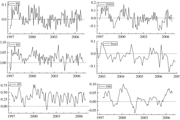
The indicators relative to all of the above models are plotted in Figure 1 which 6

shows the log-transformed IPI, the energy indicators (EE andSnam) and the raw materials (TONN) in seasonal differences, the unbounded PP andPMI.

5 Empirical results

All models presented in section 4 are estimated over a common sample 1997:7- 2005:9 (with the exception of the Gas model whose sample begins in 2002:1).

In order to evaluate in-sample correct specification the standard diagnostics are performed (the results are available upon request from the authors). The fore- casting exercise is carried out using both recursive and rolling schemes. The latter is generally used when there are concerns about turning points and biases from the use of older information. The rolling scheme is used for a sensitivity analysis with respect to the results of the combination obtained through the hierarchical procedure. The dimension of the rolling window varies with each model to account for the different time span over which the indicators are avail- able (starting in 1979 forTONN, in 1991 forIPI andPP, in 1997 forPMI, and in 2001 forSnam).

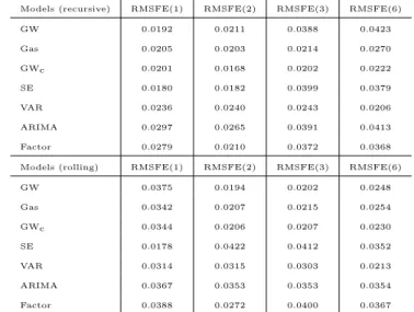
In Table 1 the RMSFE of the out-sample forecasts for each model is reported.

On the basis of these results, the models are ranked from the best to the worst for each forecast horizon (see Table 2). Different results in terms of the ranked models are found for recursive and rolling estimations respectively. With re- gards to the first-step ahead, the SE model is first ranked in both estimation frameworks, but its forecasting accuracy worsens in the successive steps ahead.

When the recursive scheme is considered, the GWcmodel shows higher rankings at several prediction steps and has a slightly better performance than the rolling estimates for h=1, 2. When six-steps ahead are considered, the VAR model is characterized by significantly higher performances and outperforms all the other models, as is generally expected. Its predictive ability slightly improves in the rolling schemes, due to the process of discarding the more dated observations in presence of the long lag structure of model equations.

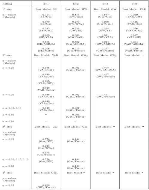
On the basis of the rank classification, the HLN test is applied to eliminate models that are encompassed by others (see Tables 3-4). Given the number of steps ahead and the estimation scheme, the number of models selected for combination depends on the significance level. The lower the significance level α, the stronger the selection becomes between competing models. As αrises, a larger number of forecasts are selected for combination. As regards the first- step ahead, at the significance level of 25% four models are selected in the both recursive (SE,GW,GWc,Gas) and rolling (SE,VAR,Gas,GWc) schemes. At lower value ofα, the selected models are reduced to three (the fourth model in each scheme is ruled out respectively) and at significance level of 1%, only the SE model is selected in both estimation frameworks.

In the recursive scheme, the selected models are GWc and SE forh=2 irrespec- tive of the significance levels; GWcand Gas forh=3 (VAR is only chosen when α= 0.25). As regards the rolling estimates, four models enter the combination forh=2 andα∈[0.05,0.25] (GW,GWc,Gas,Factor). The models based on the electricity indicator are the only ones used for the combination when h=3 and the GW model is the only selected whenα≤0.15. For the six-steps ahead, the VAR model outperforms all the other models.

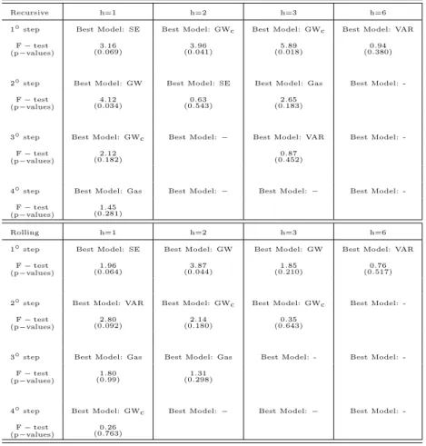
The multiple encompassing F-test would seem to confirm the HLN test findings

7

(similar results are found using the multivariate analogue Diebold-Mariano test, M S^∗, also proposed by Harvey and Newbold (2000). They are available upon request from the authors). The selection model results are reported in Table 5. The F-test is applied to each best model against all the competing models at all steps of the hierarchical procedure. For each significance level, the rejec- tion of the null hypothesis indicates that at least some of the rival models are not encompassed by the best model. As regards the one-step horizon for the recursive scheme, the F-test supports the HLN test results at each step of the procedure. Thus, the multiple encompassing test assesses the robustness of our hierarchical algorithm in selecting models that are not encompassed. Similar results are found for the rolling scheme. With respect to the second-step ahead for the recursive scheme, the F-test confirms the results based on the HLN test.

The only difference is found in the first step of the hierarchical procedure in which the F-test rejects the null hypothesis at significance level of 5% (instead of 1% as is observed in the HLN test). In the rolling scheme, for h= 1,2, the F-test results show higher probability than that one in the HLN test. Thus there is a greater tendency to accept the null hypothesis of encompassing. For h >2, multiple encompassing F-test confirms the HLN test results.

As a general result from the empirical exercise, the recursive scheme generally provides better findings in terms of forecasting accuracy. In this framework, the superiority of the hierarchical combination turns out to be substantially better when longer forecast horizons are concerned (h >1). For the first-step ahead, the forecast accuracy of the combination algorithm results only slightly better than the one obtained in the rolling scheme.

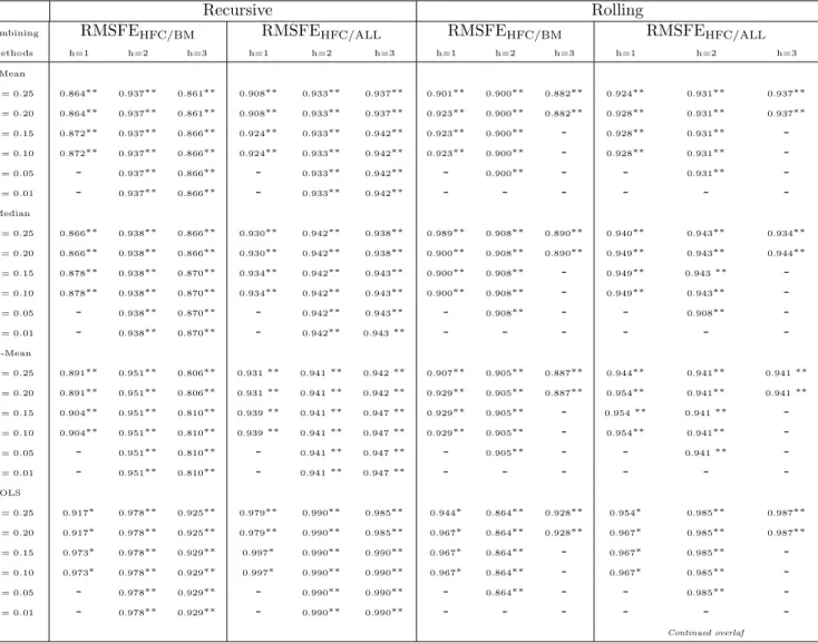
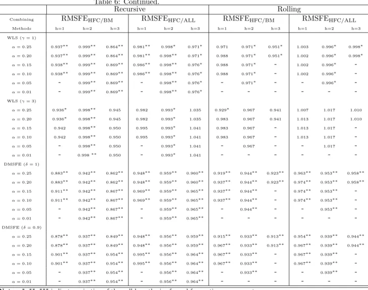
When model selection takes place, the hierarchical combination is able to out- perform both the single best model and the combination of the overall models in terms of RMSFE. In order to assess the robustness of the algorithm procedure, we evaluate the relative RMSFE, computed as a ratio between the RMSFE of the hierarchical forecast combination (HFC) and the RMSFE from both the best sin- gle model (BM) and the combination of overall models (ALL) (RMSFE_HFC/BM and RMSFE_HFC/ALLrespectively; see Table 6). Results for the six-steps ahead are not reported as the first ranked model systematically encompasses all the others regardless of the significance levels. The RMSFE indices are significantly less than one in many cases at 5%. These findings confirm the goodness of the hierarchical procedure.

Regardless of the combination methods and of the number of steps ahead, the best results in terms of relative RMSFE are obtained for higher significance levels, hence allowing for the averaging of a large number of models. At the low significance levels, very few forecasts are considered for combination and the overall forecast benefits less from the advantages of combining. The upper significance level is set at α= 0.25, since no significant improvement in terms of forecast accuracy is found using the hierarchical combination for higher sig- nificance values. Similar results are also found in Kisinbay (2007).

The performance of the several combination methods can be ranked in terms of relative RMSFE. In both schemes, the basic linear pooling methodologies (mean, median and trimmed mean) perform remarkably better than other com- bination methods (with the only exception of the OLS method in the case of rolling scheme for the RMSFE_HFC/BM and h=2). These results are consistent with the prevailing international literature and with most of the Italian em- pirical evidence. With respect to the Italian forecasting research, Bodo and

8

Signorini (1987) and Bodo, Cividini and Signorini (1991) find that the combi- nation forecasts are better than any single model in terms of the RMSFE and that the simple average methods for combination provide better results. In con- trast to this evidence, Marchetti and Parigi (2000) find that the combination of forecasts is not fully satisfactory as yields only marginal improvements when several methods of combining forecasts are used.

The relative RMSFE is also less than one in the case of discounted combination method (DMSFE) in which the weights are estimated so as to be affected by most recent past model performance (Newbold and Harvey, 2002). The worst results are obtained using the WLS method. Recent literature has stressed the poorer performance of this method for combination (Newbold, Zumwalt and Kannan, 1987).

6 Conclusions

In this paper a hierarchical procedure to increase the efficiency of forecasting combining methods is provided. The procedure considers out-of-sample fore- casts as inputs. Ericsson (1992) shows that the forecast encompassing of a given model versus the other non-nested models is a sufficient condition to min- imize RMSFE. This result is employed in our hierarchical procedure. The basic idea is to compare all forecasting models with each other using the Harvey et al. (1998) encompassing test in one direction in order to eliminate those mod- els which are encompassed by others, and subsequently to use several forecast combining methods to combine the remaining forecasts. Thus, the hierarchical procedure aims to unit model selection and model averaging methods, using larger weights for forecasts that provide information which is not contained in most of the remaining models and discounting the predictions that are encom- passed by other forecasts. The robustness of the procedure is then investigated in terms of the relative RMSFE using ISAE (Institute for Studies and Economic Analyses) short-term forecasting models for monthly industrial production in Italy. Results confirm the goodness of the hierarchical procedure.

References

Bai, J. & Ng, S. (2002). Determining the Number of Factors in Approximate Factor Models. Econometrica, 70, 191-221.

Banbura, M. & R¨unstler, G. (2007). A look into the factor model black box - publication lags and the role of hard and soft data in forecasting GDP, Working Paper Series 751, European Central Bank.

Bodo, G., Cividini, A. and Signorini, L. F. (1991). Forecasting the Italian industrial production index in real time, Journal of Forecasting, 10, 285-99.

Bodo, G. and Signorini, L. F. (1987). Short-term forecasting of the industrial production index, International Journal of Forecasting, 3, 245-9.

Bruno, G. & Lupi, C. (2004). Forecasting industrial production and the early detection of turning points. Empirical Economics, 29, 647-671.

Diebold, F.X. & Mariano, R. (1995). Comparing Predictive Accuracy. Journal of Business and Economic Statistics, 13, 253-263.

9

Diebold, F.X. & Pauly, P. (1987). Structural Change and the Combination of Forecasts. Journal of Forecasting, 6, 21-40.

Ericsson, N. R. (1992). Parameter Constancy, Mean Square Forecast Errors, and Measuring Forecast Performance: An Exposition, Extensions, and Illustration.

Journal of Policy Modelling, 4, 465-495.

Granger, C. W. J. & Ramanathan, R. (1984). Improved Methods of Combining Forecasts. Journal of Forecasting, 3, 197-204.

Harvey, D., Leybourne, S. & Newbold, P. (1997). Testing the equality of pre- diction mean squared errors. International Journal of Forecasting, 13, 281-291.

Harvey, D. I., Leybourne, S. & Newbold, P. (1998). Tests for forecast encom- passing. Journal of Business and Economic Statistics, 16, 254-259.

Harvey, D. & Newbold, P. (2000). Tests for multiple forecast encompassing, Journal of Applied Econometrics, 15, 471-482.

Hendry, D. F & Clements, M. P. (2004). Pooling of Forecasts, Econometrics Journal, volume 7, 131.

Hendry, D. F. & Krolzig, H.M. (1999). Improving on Data mining reconsidered by K.D. Hoover and S.J. Perez. Econometrics Journal, 2, 202-219.

Kisinbay, T. (2007) The Use of Encompassing Tests for Forecast Combinations.

Working paper, International Monetary Found, 264, 1-21.

Krolzig, H. M. & Hendry, D. F. (2001). Computer automation of general-to- specific model selection procedures. Journal of Economic Dynamics and Con- trol, 25, 831-866.

Marchetti, D.J. and Parigi, G. (2000). Energy consumption, survey data and the prediction of industrial production in Italy: a comparison and combination of different models, Journal of Forecasting, 19, 419-440.

Newbold, P. & Harvey, I. H. (2002) Forecast Combination and Encompassing.

In: M.P. Clements & D.F. Hendry A Companion to Economic Forecasting.

Blackwell Publishers, pp. 268-283.

Newbold, P., Zumwalt, J. K. & Kannan, S. (1987). Combining forecasts to improve earnings per share prediction: and examination of electric utilities.

International Journal of Forecasting, 3, 229-238.

R¨unstler G. & S`edillot, F. (2003). Short-term Estimates of Euro Area Real Gdp by Means of Monthly Data, ECB Working Paper, n. 276.

Stock, J. H. & Watson, M. W. (1998). Diffusion indexes. Working Paper 6702, NBER, 1-65.

Stock, J. H. & Watson, M. W. (2002). Macroeconomic forecasting using diffu- sion indices. Journal of Business and Economic Statistics, 20, 147-162.

Stock J. H. & Watson, M. W. (2004). Combination forecasts of output growth in a seven-country data set. Journal of Forecasting, 23, 405-430.

10

1997 2000 2003 2006 0.0

0.1 ^IPI

1997 2000 2003 2006

−0.1 0.0 0.1

0.2 _TONN

1997 2000 2003 2006

0.00 0.05 0.10 EE

1997 2000 2003 2006

−0.05 0.00 0.05

0.10 PMI

2003 2004 2005 2006 2007

−0.1 0.0

0.1 Snam

1997 2000 2003 2006

0.00 0.25 0.50 0.75 ^PP

Figure 1: Indicators for forecasting models.

11

Table 1: Forecast errors measures. Recursive and Rolling estimation

Models (recursive) RMSFE(1) RMSFE(2) RMSFE(3) RMSFE(6)

GW 0.0192 0.0211 0.0388 0.0423

Gas 0.0205 0.0203 0.0214 0.0270

GWc 0.0201 0.0168 0.0202 0.0222

SE 0.0180 0.0182 0.0399 0.0379

VAR 0.0236 0.0240 0.0243 0.0206

ARIMA 0.0297 0.0265 0.0391 0.0413

Factor 0.0279 0.0210 0.0372 0.0368

Models (rolling) RMSFE(1) RMSFE(2) RMSFE(3) RMSFE(6)

GW 0.0375 0.0194 0.0202 0.0248

Gas 0.0342 0.0207 0.0215 0.0254

GWc 0.0344 0.0206 0.0207 0.0230

SE 0.0178 0.0422 0.0412 0.0352

VAR 0.0314 0.0315 0.0303 0.0213

ARIMA 0.0367 0.0353 0.0353 0.0354

Factor 0.0388 0.0272 0.0400 0.0367

Notes: numbers in parentheses are the steps-ahead forecast.

Table 2: Rank Classification. Recursive and Rolling estimation

Recursive Rolling

rank h=1 h=2 h=3 h=6 h=1 h=2 h=3 h=6

1 SE GWc GWc VAR SE GW GW VAR

2 GW SE Gas GWc VAR GWc GWc GWc

3 GWc Gas VAR Gas Gas Gas Gas GW

4 Gas Factor Factor Factor GWc Factor VAR Gas

5 VAR GW GW SE ARIMA VAR ARIMA SE

6 Factor VAR SE ARIMA GW ARIMA Factor ARIMA

7 ARIMA ARIMA ARIMA GW Factor SE SE Factor

12

Table 3: Encompassing (HLN) test results. Recursive estimation.

Recursive h=1 h=2 h=3 h=6

1◦step Best Model: SE Best Model: GWc Best Model: GWc Best Model: VAR p−values

(Models)

0.150

(SE/GW) 0.004

(GWc/GW) 0.220

(Gwc/GW) 0.278

(VAR/GW) 0.112

(SE/Gas) 0.073

(GWc/Gas) 0.005

(GWc/Gas) 0.422

(VAR/Gas) 0.103

(SE/GWc) 0.061

(GWc/SE) 0.230

(GWc/SE) 0.286

(VAR/Gwc) 0.183

(SE/VAR) 0.561

(GWc/VAR) 0.375

(GWc/VAR) 0.336

(VAR/SE) 0.426

(SE/ARIMA) 0.794

(GWc/ARIMA) 0.009

(GWc/ARIMA) 0.381

(VAR/ARIMA) 0.052

(SE/Factor) 0.880

(GWc/Factor) 0.465

(GWc/Factor) 0.261

(VAR/Factor) 2◦step Best Model: GW Best Model: SE Best Model: Gas Best Model: -

p−values (Models)

α= 0.25 0.167

(GW/Gas) 0.508

(SE/GW) 0.194

(Gas/GW) 0.033

(GW/GWc) 0.409

(SE/Gas) 0.190

(Gas/SE) 0.031

(GW/VAR) 0.420

(Gas/ARIMA) 0.075

(GW/Factor)

α= 0.20 0.167

(GW/Gas) 0.508

(SE/GW) 0.420

(Gas/ARIMA) 0.033

(GW/GWc) 0.409

(SE/Gas) 0.031

(GW/VAR) 0.075 (GW/Factor)

α= 0.15 0.167

(GW/Gas) 0.508

(SE/GW) 0.420

(Gas/ARIMA) 0.033

(GW/GWc) 0.409

(SE/Gas) 0.075

(GW/Factor)

α= 0.10 0.075

(GW/Factor) 0.508

(SE/GW) 0.420

(Gas/ARIMA) 0.490

(SE/Gas)

α= 0.05,0.01 - ^0.508

(SE/GW) 0.420

(Gas/ARIMA)

3◦step Best Model: GWc Best Model: - Best Model: VAR Best Model: -

p−values (Models)

α= 0.25 0.220

(GWc/Gas) 0.373

(VAR/GW) 0.322

(GWc/VAR) 0.279

(VAR/SE) 0.151

(GWc/Factor)

α= 0.20 0.220

(GWc/Gas) 0.322 (GWc/VAR)

0.151 (GWc/Factor) α= 0.15,0.10 0.151

(GWc/Factor)

4◦step Best Model: Gas Best Model: - Best Model: - Best Model: -

p−values (Models)

α= 0.25,0.20 0.273 (Gas/Factor)

13

Table 4: Encompassing (HLN) test results. Rolling estimation.

Rolling h=1 h=2 h=3 h=6

1◦step Best Model: SE Best Model: GW Best Model: GW Best Model: VAR p−values

(Models) 0.154

(SE/GW) 0.874

(GW/Gas) 0.657

(GW/Gas) 0.269

(VAR/GW) 0.070

(SE/Gas) 0.279

(GW/GWc) 0.290

(GW/GWc) 0.546

(VAR/Gas) 0.243

(SE/GWc) 0.256

(GW/SE) 0.274

(GW/SE) 0.256

(VAR/Gwc) 0.065

(SE/VAR) 0.306

(GW/VAR) 0.331

(GW/VAR) 0.597

(VAR/SE) 0.595

(SE/ARIMA) 0.502

(GW/ARIMA) 0.214

(GW/ARIMA) 0.304

(VAR/ARIMA) 0.206

(SE/Factor) 0.019

(GW/Factor) 0.197

(GW/Factor) 0.359

(VAR/Factor) 2◦step Best Model: VAR Best Model: GWc Best Mode: GWc Best Model: -

p−values (Models)

α= 0.25 0.086

(VAR/GW) 0.007

(GWc/Factor) 0.707 (GWc/ARIMA) 0.049

(VAR/Gas) 0.467

(GWc/Factor) 0.085

(VAR/GWc) 0.029 (VAR/Factor)

α= 0.20 0.086

(VAR/GW) 0.007

(GWc/Factor) 0.467 (GWc/Factor) 0.049

(VAR/Gas)

α= 0.15,0.10 0.049

(VAR/Gas) 0.007

(GWc/Factor)

α= 0.05 - ^0.007

(GWc/Factor)

α= 0.01 - -

3◦step Best Model: Gas Best Model: Gas Best Model: - Best Model: -

p−values (Models)

α= 0.25 0.776

(Gas/GW) 0.144

(Gas/Factor) 0.243

(Gas/GWc) 0.075 (Gas/Factor) α= 0.20,0.15,0.10 0.776

(Gas/GW) 0.144

(Gas/Factor)

α= 0.05 0.144

(Gas/Factor)

4◦step Best Model: GWc Best Model- ^{Best Model}- ^{Best Model}-

p−values (Models)

α= 0.25 0.600

(GWc/Factor)

14

Table 5: Multiple encompassing test results. Recursive and Rolling estimation.

Recursive h=1 h=2 h=3 h=6

1◦step Best Model: SE Best Model: GWc Best Model: GWc Best Model: VAR F−test

(p−values) 3.16

(0.069) 3.96

(0.041) 5.89

(0.018) 0.94

(0.380)

2◦step Best Model: GW Best Model: SE Best Model: Gas Best Model: - F−test

(p−values) 4.12

(0.034) 0.63

(0.543) 2.65

(0.183)

3◦step Best Model: GWc Best Model:− Best Model: VAR Best Model: - F−test

(p−values) 2.12

(0.182) 0.87

(0.452)

4◦step Best Model: Gas Best Model:− Best Model:− Best Model: - F−test

(p−values) 1.45 (0.281)

Rolling h=1 h=2 h=3 h=6

1◦step Best Model: SE Best Model: GW Best Model: GW Best Model: VAR F−test

(p−values) 1.96

(0.064) 3.87

(0.044) 1.85

(0.210) 0.76

(0.517)

2◦step Best Model: VAR Best Model: GWc Best Model: GWc Best Model: - F−test

(p−values) 2.80

(0.092) 2.14

(0.180) 0.35

(0.643)

3◦step Best Model: Gas Best Model: Gas Best Model: - Best Model: - F−test

(p−values) 1.80

(0.99) 1.31

(0.298)

4◦step Best Model: GWc Best Model:− Best Model:− Best Model: - F−test

(p−values) 0.26 (0.763)

15