DISSERTATION
zur Erlangung des akademischen Grades doctor rerum politicarum
(Dr. rer. pol.)
im Fach Wirtschaftswissenschaft eingereicht an der
Wirtschaftswissenschaftliche Fakultät Humboldt-Universität zu Berlin
von
Frau M.Sc. Ying Chen
geboren am 08.12.1975 in Kaifeng, VR China
Präsident der Humboldt-Universität zu Berlin:
Prof. Dr. Christoph Markschies
Dekan der Wirtschaftswissenschaftliche Fakultät:
Prof. Oliver Günther, Ph.D.
Gutachter:
1. Prof. Dr. Wolfgang Härdle 2. Prof. Dr. Vladimir Spokoiny
eingereicht am: 15. Oktober 2006
Tag der mündlichen Prüfung: 9. Januar 2007
Over recent years, study on risk management has been prompted by the Basel committee for the requirement of regular banking supervisory. There are however limitations of many risk management methods: 1) covariance estimation relies on a time-invariant form, 2) models are based on unrealistic distributional assumption and 3) numerical problems appear when applied to high-dimensional portfolios.
The primary aim of this dissertation is to propose adaptive methods that overcome these limitations and can accurately and fast measure risk expo- sures of multivariate portfolios. The basic idea is to first retrieve out of high-dimensional time series stochastically independent components (ICs) and then identify the distributional behavior of every resulting IC in uni- variate space. To be more specific, two local parametric approaches, local moving window average (MWA) method and local exponential smoothing (ES) method, are used to estimate the volatility process of every IC under the heavy-tailed distributional assumption, namely ICs are generalized hy- perbolic (GH) distributed. By doing so, it speeds up the computation of risk measures and achieves much better accuracy than many popular risk management methods.
Keywords:
Risk management, Heavy-tailed distribution, Local parametric methods, High-dimensional data analysis
In den vergangenen Jahren ist die Untersuchung des Risikomanagements vom Baselkomitee angeregt, um die Kredit- und Bankwesen regelmäßig zu auf- sichten. Für viele multivariate Risikomanagementmethoden gibt es jedoch Beschränkungen von: 1) verlässt sich die Kovarianzschätzung auf eine zei- tunabhängige Form, 2) die Modelle beruhen auf eine unrealistischen Vertei- lungsannahme und 3) numerische Problem, die bei hochdimensionalen Daten auftreten.
Es ist das primäre Ziel dieser Doktorarbeit, präzise und schnelle Methoden vorzuschlagen, die diesen Beschränkungen überwinden. Die Grundidee be- steht darin, zuerst aus einer hochdimensionalen Zeitreihe die stochastisch unabhängigen Komponenten (IC) zu extrahieren und dann die Verteilungs- parameter der resultierenden IC beruhend auf eindimensionale Heavy-Tailed Verteilungsannahme zu identifizieren. Genauer gesagt werden zwei lokale pa- rametrische Methoden verwendet, um den Varianzprozess jeder IC zu schät- zen, das lokale Moving Window Average (MVA) Methode und das lokale Exponential Smoothing (ES) Methode. Diese Schätzungen beruhen auf der realistischen Annahme, dass die IC Generalized Hyperbolic (GH) verteilt sind. Die Berechnung ist schneller und erreicht eine höhere Genauigkeit als viele bekannte Risikomanagementmethoden.
Schlagwörter:
Risikomanagement, Heavy-Tailed Verteilung, Lokale parametrische Methoden, Hochdimensionale Datenanalyse
I Basic Concepts 1
1 Introduction 2
2 Risk analysis 13
2.1 Risk: classification and definition . . . 13
2.2 Risk measures . . . 15
2.3 Requirements on risk analysis . . . 16
2.4 Review of popular risk management models: pros and cons . . 18
2.4.1 Univariate risk management model . . . 19
2.4.2 Multivariate risk management models . . . 20
2.5 Adaptive risk management models . . . 22
II Adaptive Risk Management - Univariate Models 25
3 Adaptive risk management 1: GHADA 26 3.1 Introduction . . . 263.2 GHADA technique . . . 30
3.2.1 Generalized hyperbolic distribution . . . 30
3.2.2 Adaptive volatility estimation . . . 33
3.3 Simulation study . . . 36
3.4 Real data analysis . . . 40
3.4.1 Data set . . . 40
3.4.2 Risk analysis . . . 44
3.5 Conclusion . . . 50
3.6 Appendix . . . 52
4 Adaptive risk management 2: LESGH 55 4.1 Introduction . . . 55
4.2 Volatility modeling. Local parametric approach . . . 59
4.2.1 Local parametric modeling . . . 60 iv
4.2.3 Some properties of the quasi MLE in the homogeneous
situation for sub-Gaussian innovations . . . 63
4.2.4 Canonical parametrization . . . 64
4.2.5 Problem of adaptive estimation . . . 65
4.2.6 Spatial aggregation of local likelihood estimates (SSA) 66 4.3 Parameter choice and implementation details . . . 67
4.3.1 Example of the smoothing parameter set . . . 67
4.3.2 “Aggregation” kernel . . . 68
4.3.3 Critical values . . . 68
4.3.4 Sequential choice of the critical values by Monte Carlo simulations . . . 70
4.3.5 Sensitivity analysis. Numerical study . . . 71
4.3.6 Parameter tuning by minimizing forecast errors . . . . 75
4.4 Quasi maximum likelihood estimation under normal inverse Gaussian (NIG) distributional assumption . . . 76
4.5 Numerical study . . . 78
4.5.1 Simulation study . . . 79
4.5.2 Application to risk analysis . . . 84
III Adaptive Risk Management - Multivariate Mod- els 89
5 Adaptive risk management 3: ICVaR 90 5.1 Introduction . . . 905.2 ICVaR methodology . . . 94
5.2.1 Basic model . . . 94
5.2.2 ICA: Properties and Estimation . . . 95
5.3 Simulation Study . . . 101
5.4 Real data analysis . . . 103
5.4.1 Exchange rate . . . 103
5.4.2 German stock portfolio . . . 107
5.5 Conclusion . . . 116
6 Adaptive risk management 4: GHICA 120 6.1 Introduction . . . 120
6.2 GHICA Methodology . . . 124
6.2.1 Independent component analysis (ICA) and FastICA approach . . . 125
v
6.2.3 Normal inverse Gaussian (NIG) distribution and fast
Fourier transformation (FFT) . . . 131
6.3 Covariance estimation with simulated data . . . 133
6.4 Risk management with real data . . . 137
6.4.1 Data analysis 1: DAX portfolio . . . 139
6.4.2 Data analysis 2: Foreign exchange rate portfolio . . . . 140
Bibliography 142
Selbständigkeitserklärung 152
vi
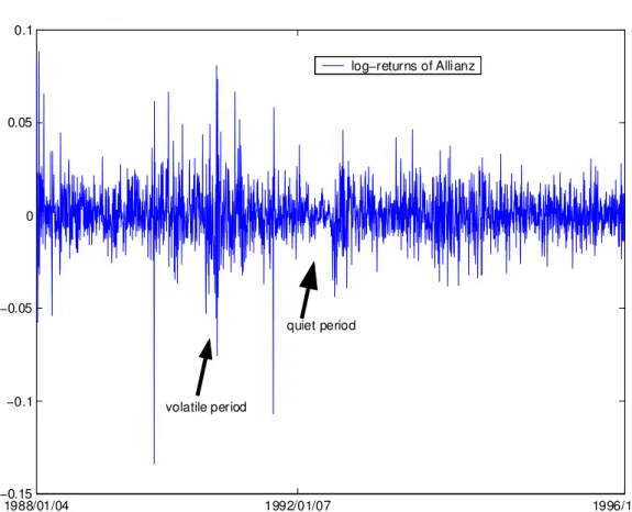
1.1 Log-returns of the German stock Allianz from 1988/01/04 to 1996/12/30. Data source: FEDC (http://sfb649.wiwi.hu- berlin.de) . . . 4 1.2 Volatility estimates of the German stock Allianz over three
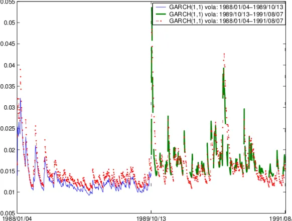
time periods: σ2(t) = ω + αx2(t − 1) +βσ2(t − 1). Data source: FEDC (http://sfb649.wiwi.hu-berlin.de) . . . 7 1.3 Density comparisons of the standardized returns in log scale
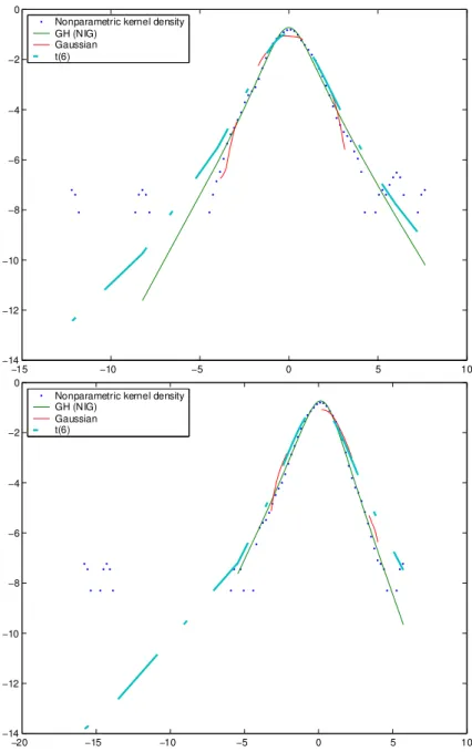
based on the Allianz stock (top) and the DAX portfolio (bot- tom) with a static weight b(t) = unit(1/20). Time interval:
1988/01/04 - 1996/12/30. The nonparametric kernel density is considered as benchmark. The GH distributional parameters are respectively GH(−0.5,1.01,0.05,1.11,−0.03) for the Al- lianz and GH(−0.5,1.21,−0.21,1.21,0.24) for the DAX port- folio. Data source: FEDC (sfb649.wiwi.hu-berlin.de). . . 10 1.4 Procedure of adaptive risk management models. . . 11 2.1 Empirical density of the German stock Allianz from 1988/01/04
to 1996/12/30. The values of VaR (average value: 0.035) and ES (0.044) correspond to a probability level pr = 1% over a target time horizon h= 1. . . 16 3.1 Density estimation of the daily DEM/USD standardized re-
turns from 1979/12/01 to 1994/04/01 (3719 observations).
The log scale of the estimation is displayed on the right panel.
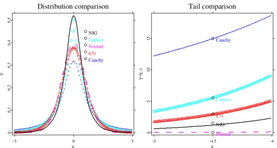
The nonparametric kernel density estimate is considered as benchmark. The bandwidth is h0 ≈0.54. Data source: FEDC (http://sfb649.wiwi.hu-berlin.de). . . 28 3.2 Tail-behavior of five standardized distributions: NIG distri-
bution, standard Gaussian distribution, Student-tdistribution with degrees of freedom 5, Laplace distribution and Cauchy distribution. . . 31
vii
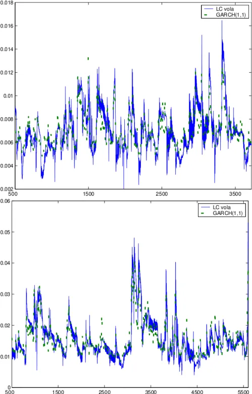
for σ3(t). The involved parameters are γ = 0.5, m0 = 5 and the starting point t0 = 201. The volatility processes are esti- mated by using the GARCH(1,1) model and the local constant (LC) model respectively. . . 38 3.4 Volatility estimation based on the DEM/USD rate (top) and
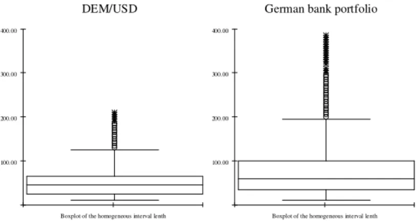
the German bank portfolio (bottom). The parameters in the local constant models are t0 = 501, m0 = 5, z0 = 1.06 for the DEM/USD data and z0 = 1.23 for the German bank portfolio data. . . 42 3.5 Boxplots of the homogeneous interval length w.r.t. the DEM/USD
exchange rates (left) and the German bank portfolio data (right). 43 3.6 Density estimations of the standardized DEM/USD returns
under various distributional assumption. The density of the LC-based standardized returns is identified on the top whereas that of the GARCH(1,1)-based standardized returns is illus- trated on the bottom. The corresponding log densities are displayed on the right side. The GH distributional parame- ters are listed in Table 3.5. . . 45 3.7 Density estimations of the standardized German bank port-
folio returns under various distributional assumption. The density of the LC-based standardized returns is identified on the top whereas that of the GARCH(1,1)-based standardized returns is illustrated on the bottom. The corresponding log densities are displayed on the right side. The GH distribu- tional parameters are listed in Table 3.5. . . 46 3.8 Quantiles estimated based on the past 500 standardized re-
turns of the exchange rate. From the top the evolving HYP quantiles for pr = 0.995, pr = 0.99, pr = 0.975, pr = 0.95, pr = 0.90, pr = 0.10, pr = 0.05, pr = 0.025, pr = 0.01, pr = 0.005. . . 47 3.9 Time plots of the VaR forecasts on the base of the DEM/USD
returns for the intervalt ∈[3000,3719] atpr = 0.05(top) and pr = 0.01 (bottom). The volatility is estimated by using the local constant model and the standardized returns are respec- tively identified in the GH (HYP), Gaussian and Studnet-t distributional frameworks. . . 51
viii
0.752 versus η = 0.94 is applied. The log returns from 1998/03/05 to 1998/07/24 are displayed as dots. . . 57 4.2 Sequences of critical values zk for r = 0.3, r = 0.5, r = 0.7
and r = 1. . . 73 4.3 Sequences of critical values zk for α = 0.5, α = 1 and α =
1.5. . . 74 4.4 Sequences of critical values zk for a= 1.25 and a= 1.1 w.r.t.
the smoothing parameter ηk for k= 1,· · ·, K. . . 75 4.5 Sequences of critical values zk for c= 0.01 and c= 0.001. . 76 4.6 Estimation based on one realized simulation data with εt ∼
N(0,1). The ES (η = 0.94), LMS and SSA estimates and the generated variance process are depicted on the top. The absolute errors of the LMS and SSA estimates are compared with the ES estimates w.r.t. {ηk} for k = 2,· · ·,15. . . 80 4.7 The boxplots of the RAEs of the SSA, LMS and ES with ηk
for k = 2,· · ·, K. . . 81 4.8 The average RAEs of the SSA (blue and solid curve) and LMS
(cyan and dotted curve) estimates through the 100 simulations. 82 4.9 Estimation based on one realized simulation data with εt ∼
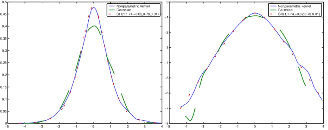
NIG(1.340,−0.015,1.337,0.010). The ES (η = 0.94) and SSA (p = 0.25) estimates and the generated variance process are depicted. . . 83 5.1 Graphical comparison of density estimations based on the stan-
dardized DEM/USD returns from 1979/12/01 to 1994/04/01 (3719 observations). The nonparametric kernel density es- timations (solid curve) are considered as benchmarks. No- tice that the nonparametric density estimations result distinct forms w.r.t. different standardization, or more details, w.r.t.
different volatility estimation methods. The HS-RM based density estimation is the dotted curve on the left panel whereas the HS-ESt(15)based estimation is displayed on the right. The corresponding GARCH(1,1) process is: ˆσx2(t) = 1.65∗10−6 + 0.07x2(t−1) + 0.89ˆσx2(t−1).The GHADA technique with the local constant volatility process and the GH(1,1.74,−0.02,0.78,0.01) density estimation is displayed on the middle panel. Data source: FEDC(http://sfb649.wiwi.hu-berlin.de). . . 92
ix
on the middle row where the linear transformation matrixW is estimated based on 3 German stocks’ returns: Allianz, BASF and Bayer from 1974/01/02 to 1996/12/30. The time series of the estimated ICs are displayed on the bottom. . . 97 5.3 Comparison of the true negentropy (solid line) and its approxi-
mations (a: red and dashed, b: blue and dotted) of a simulated Gaussian mixture variable: pN(0,1)+(1−p)N(1,4)forp∈[0,1].100 5.4 ACF plots of the log returns of the DEM/USD (left) and the
GBP/USD (right) are displays on the top. Below are the ACF plots of the estimated IC series: IC1 (left) and IC2 (right). . . 104 5.5 Adaptive volatility processes of the FX ICs. . . 105 5.6 Comparison of the nonparametric joint density (black) of the
returns of the exchange rates and the product (blue) of the HYP marginal densities of two ICs. The red surface is the Gaussian fitting with the same covariance as the returns of the exchange rates. . . 106 5.7 VaR time plot of the exchange rate portfolio with trading
strategy b4 = (−2,1)> at risk level pr = 0.5%. Three risk management models are implemented: ICVaR (HYP), HS-RM and HS-ESt(14). . . 111 5.8 Density estimation of the first IC on the basis of the German
stock portfolio. The HYP fit is displayed as a straight curve and the nonparametric density estimation is plotted by a dot- ted curve. . . 112 5.9 Density estimation of the first IC on the basis of the German
stock portfolio. The NIG fit is displayed as a straight curve and the nonparametric density estimation is plotted by a dot- ted curve. . . 114 5.10 VaR time plots of the German stock portfolio with the equal
weights. Three risk management models are implemented:
ICVaR (NIG), HS-RM and HS-ESt(19). The risk levels are respectively pr = 5%(top) and 0.5% (bottom). . . 117 5.11 VaR time plots of the German stock portfolio with the equal
weights. Three risk management models are implemented:
ICVaR (NIG), HS-RM and HS-ESt(19). The risk level ispr = 0.1%. . . 119
x
tom) with static weights b(t) = unit(1/20). Time interval:
1988/01/04 - 1996/12/30. The nonparametric kernel density is considered as benchmark. The GH distributional parameters are respectively GH(−0.5,1.01,0.05,1.11,−0.03) for the Al- lianz and GH(−0.5,1.21,−0.21,1.21,0.24) for the DAX port- folio. Data source: FEDC (http://sfb649.wiwi.hu-berlin.de). . 122 6.2 Ordered eigenvalues of the generated covariance matrices. . . . 134 6.3 Structure shifts of the generated covariance through time. No-
tice that there are shifts among matrices not up-and-down movements. . . 135 6.4 Realized estimates of Σ(2,5) based on the GHICA and DCC
methods. The generated data consists of 50 NIG distributed components. . . 137 6.5 Boxplot of the proportion
P
i
P
j1(RAE(i,j)≤1)
d×d fori, j = 1,· · ·, d.
Hered= 50and the proportions on the base of100simulations are considered. . . 138 6.6 One day log-returns of the DAX portfolio with the static trad-
ing strategy b(t) = b(1). The VaRs are from 1975/03/17 to 1996/12/30 at pr = 0.5% w.r.t. three methods, the GHICA, the RiskMetrics and the t(6). Part of the VaR time plot is enlarged and displayed on the bottom. . . 141
xi
1.1 ML estimates of the GARCH(1,1) model on the base of the German stock Allianz. The standard deviation of the esti- mates are reported in parentheses. . . 6 2.1 Traffic light as a factor of the exceeding amount, cited from
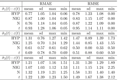
Franke, Härdle and Hafner (2004). . . 17 3.1 Alternative risk management models. . . 29 3.2 Descriptive statistics of the two criteria for accuracy of estima-
tion: RMAE and RMSE. Two volatility models: local constant (LC) (γ = 0.5 and m0 = 5) and GARCH(1,1) models are ap- plied to estimate three generated volatility processes. Four kinds of random variables are used to generate the observa- tions: HYP(2,0,1,0), NIG(2,0,1,0), N(0,1) and t(6). . . 39 3.3 Mean of the detection steps w.r.t. jumps over200simulations.
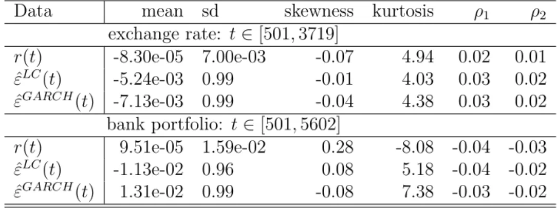
Two methods are implemented to estimate volatility: the lo- cal constant (LC) model with m0 = 2 and m0 = 5 and the GARCH(1,1) model. The standard deviations of the detec- tion steps are put in parentheses. Two jumps w.r.t. σ1t at t = 300 and t= 600 and two jumps w.r.t. σ2t at t = 400 and t= 750 are considered. . . 40 3.4 Descriptive statistics for the daily standardized residuals of
the exchange rate data and bank portfolio data. . . 41 3.5 Distributional parameters of the standardized residuals w.r.t.
the local constant (LC) volatility and the GARCH(1,1) volatil- ity of the DEM/USD data and the German bank portfolio data. 43
xii
reported as well. The likelihood ratio (LR) test is asymptoti- callyχ2(1)distributed. The critical values are 3.84 (95%) and 6.63 (99%) respectively. * indicates that the risk management model is rejected at 95% confidence level. Notice that NAN for LR is due to the empty set of exceptions. . . 49 4.1 ML estimates of the GARCH(1,1) model. The standard devi-
ation of the estimates are reported in parentheses. . . 58 4.2 Critical values of the SSA and LMS methods w.r.t. the default
choice: c= 0.01, a= 1.25, η1 = 0.6, r = 0.5 and α= 1. . . 72 4.3 Sensitivity analysis: comparison of the critical values zk. . . . 73 4.4 Average estimation errors of the 100 simulation data sets with
εt ∼ N(0,1), by which various estimation methods and the different parameters analyzed in the sensitivity analysis and used in the SSA estimation are considered. SSA2 means the SSA with the critical values based on forecasting errors (h = 1). In the ES, η= 0.94 is applied. . . 81 4.5 Average estimation errors of the 100 NIG data sets w.r.t. dif-
ferent values of p, by which p = 0.25 is default choice in our study. The row p= 0.25∗ is based on the critical values com- puted for the Gaussian case. The true Cp = E|εt|2p and the estimated Cˆp are reported. In the ES, η= 0.94 is applied. . . 84 4.6 Descriptive statistics of the real data. The critical value of the
KPSS test without trend is 0.347 (90%). . . 85 4.7 Risk analysis of the real data. The exceptions are marked in
green, yellow or red according to the traffic light rule. An internal model is accepted if it is in the green zone. The best results to fulfill the regulatory requirement are marked by r. The recommended method to the investor is marked by i. For the internal supervisory, we recommend the method marked by s. . . 88 5.1 ML estimatorsαˆj andβˆj of the estimated ICs, the parameters
of the true ICs and the MAE (unit: 10−2). . . 102 5.2 Descriptive statistics of the log returns and the two estimated
indpendent processes of the DEM/USD and GBP/USD rates. 103 5.3 Identified GH parameters of the estimated ICs. . . 106 5.4 Descriptive statistics of daily empirical quantile estimates: b =
(1,1)>, MC simulation with M = 10000, N = 100,T = 1000. . 108 xiii
5.6 Descriptive statistics of daily empirical quantile estimates: b = (−1,2)>, MC simulation with M = 10000, N = 100,T = 1000. 109 5.7 Descriptive statistics of daily empirical quantile estimates: b =
(−2,1)>, MC simulation with M = 10000, N = 100,T = 1000. 109 5.8 Backtesting of the VaR forecast of the exchange portfolios:
MC simulation with M = 10000, N = 100, T = 1000. ∗ indicates the model is rejected at 99% confidence level. . . 110 5.9 Descriptive statistics of the 20-dimensional German stock port-
folio. . . 113 5.10 HYP and NIG parameters estimates of the German stock port-
folio. . . 113 5.11 Descriptive statistics of quantile estimates: MC simulation
with M = 10000, N = 100, T = 1000. . . 115 5.12 Descriptive statistics of quantile estimates: MC simulation
with M = 10000, N = 100, T = 1000. . . 115 5.13 Backtesting of the VaR forecasts of the German stock portfo-
lios: MC simulation with M = 10000, N = 100, T = 1000. * indicates the rejection at 99% level. . . 118 6.1 Risk analysis of the DAX portfolios with two static trading
strategies. The concerned forecasting interval is h = 1 (top) or h = 5 (bottom) days. The best results to fulfill the reg- ulatory requirement are marked by r. The method preferred by investor is marked by i. For the internal supervisory, the method marked by s is recommended. . . 140 6.2 Risk analysis of the dynamic exchange rate portfolio. The best
results to fulfill the regulatory requirement are marked by r. The recommended method to the investor is marked byi. For the internal supervisory, we recommend the method marked bys. . . 143
xiv
Basic Concepts
1
Introduction
After the breakdown of the Bretton Woods fixed exchange rate system in 1971, financial markets have become much more volatile than before. The following boom of financial derivatives accelerated the turbulence of the mar- kets. Under such a situation, Basel committee on banking regulations and supervisory was founded by central-bank governors of the Group of ten coun- tries in 1974. The main goals of the Basel committee are to secure capital adequacy and control market risks of financial institutions. Despite the care- ful and strong regulatory, losses in trading financial instruments astonished the world due to the suddenness and the extremely large amount. For ex- ample, loss in trading financial derivatives totaled 28billion US Dollar from 1987 to 1988, see [Jor01]. To alleviate the extreme market risks, Basel accord has asked financial institutions, mainly banks, to deposit capital of risk assets as risk charge. The standard rule has changed from the beginning “8% rule”, i.e. capital reserved should be larger or equal to 8% of the risk-weighted assets, to the recent allowance of using “internal model”, i.e. risk charge is decided based on a verified quantitative model used by the financial institu- tion. Unfortunately, extreme losses are continuously observed in the market and tend to involve even larger amount of capital than before. Merely the loss of Barings has an amount of 1330 million US Dollar in trading stock index futures in 1995. These observations arise the questions: Whether the popular risk management models are appropriate for measuring risk expo- sures in the more and more sophisticated financial markets and How the risk management models can be improved.
It is important to investigate features of financial series before measur- ing its risk. Financial series shares a number of stylized facts such as non- stationary property of stock prices, volatility clustering fact and heavy-tailed distribution, see [Fam65] and [Pag96]. We here demonstrate these features on the base of the German stock Allianz from 1988/01/04 to 1996/12/30. Given
2
the observed stock price s(t), the Dickey-Fuller test is to check whether that the stock price follows a random walks(t) =c+s(t−1)+εs(t)with some con- stantcand stochastic innovations εs(t). We refer to [DF79] for details of this unit root test. With a value of −3.22we can not reject the non-stationarity hypothesis at the 5% level since the corresponding critical value is −3.41.
The test w.r.t. log-returns x(t) = log{s(t)/s(t−1)}, on the contrary, rejects the non-stationarity hypothesis. For notational simplification, we use return to express log-return in this thesis. Notice that the rejection of the unit root test only states that the first order difference of the stock price does not follow random walk. The rejection is not sufficient to say that the return process is stationary, i.e. with at least the same mean and variance. In fact, it is observed that variance is changing through time. To be more specific, large returns tend to be followed by large returns, of either sign, and small changes tend to be followed by small changes. This phenomenon was first observed by [Man63] and is famous as “volatility clustering” feature. It is displayed in Figure 1.1, where the series changes between volatile scene and relative quiet scene through time. It is rational to surmise that a large variance exists in the volatile period and a small variance is for the quiet period. Although the variance of the return process is time varying, it is supposed that the standardized returnsx(t)/Var[x(t)]have a time-homogeneous variance with expected value of 1. Furthermore, two empirical high order moments, skew- ness and kurtosis, of the standardized returns are with values of −0.177 and 12.077. These values indicate that the return process has an asymmetric distribution and heavy tails relative to the Gaussian random variable with skewness = 0 and kurtosis = 3.
In accordance with these empirical features, financial risks are typically mapped into a stochastic framework:
x(t) = Σ1/2x (t)εx(t), (1.1) wherex(t)∈IRdare risk factors, e.g. returns of ad-dimensional portfolio, the covarianceΣx(t)is time-dependent and will be filtered from the past observa- tions{x(1),· · ·, x(t−1)}. The stochastic innovationsεx(t)∈IRdare assumed to be independent and identical distributed (i.i.d.) with E[εxj(t)|Ft−1] = 0 and E[ε2xj(t)|Ft−1] = 1 for j = 1,· · ·, d. The popular risk measures such as value at risk (VaR) and expected shortfall (ES) are calculated based on the estimated joint density of the risk factors x(t), therefore, the practical risk management decisions inherently rely on out-of-sample covariance forecasts and innovations’ distributional identification, indicated by (1.1).
Many methodologies have been contributed to deal with these two tasks.
In spite of theoretical and empirical achievements, they are often not uni- formly applicable in risk management due to three limitations, see [Bol01].
Figure 1.1: Log-returns of the German stock Allianz from 1988/01/04 to 1996/12/30. Data source: FEDC (http://sfb649.wiwi.hu-berlin.de)
1. Fixed form in covariance estimation: The covariance estimation methods normally rely on a fixed parametric regression form, namely the form is time-invariant. Such a static assumption is numerically tractable but may induce large estimation errors. Since it often ob- serves structure shifts in the markets, which are driven by e.g. policy adjustments or economic changes. The static form has less flexibility to react to these shifts, and therefore, is weak to match covariance movement in a meaningful way.
2. Gaussian distributional assumption: The innovations are often assumed to be Gaussian distributed. This assumption gives fast and explicit results in the calculation, but the Gaussian distribution has relatively lighter tails than the empirical one. In risk management, risk measures are however calculated based on the tail part of the identified distribution. Therefore this Gaussian assumption costs too much in losing accuracy.
3. Numerical problem due to high-dimensionality: Last but not least, it is difficult to implement the popular models in high-dimensional analysis. Although large dimensional portfolios are actively traded by many financial institutions. The problem is that an appropriate dimen- sional reduction method is lacking in risk management.
Now let us give more details on these three limitations and briefly explain our ideas. First, two covariance estimation methods, the moving window average (MWA) method and the exponential smoothing (ES) method, are in particular desirable in practice since they are successful in reflecting the volatility clustering fact of financial series with simple forms:
MWA: Σx(t) = 1 M
( M X
m=0
x(t−m−1)x>(t−m−1)
)
, M ≤t−2 ES: Σx(t) =
( ∞ X
m=0
ηmx(t−m−1)x>(t−m−1)
)
/
( ∞ X
m=0
ηm
)
, η∈[0,1]
Notice that the ARCH and GARCH models in [Eng82] and [Bol86] can be considered as the variations of the ES method:
Σx(t) = ω+αx(t−1)x>(t−1) +βΣx(t−1)
= ω
1−β +α
∞
X
m=0
βmx(t−m−1)x>(t−m−1)
time period ωˆ αˆ βˆ 1988/01/04-1989/10/13 8.63e-06 (6.36e-06) 0.07 (0.03) 0.87 (0.05) 1989/10/13-1991/08/07 6.54e-06 (2.95e-06) 0.17 (0.07) 0.61 (0.12) 1988/01/04-1991/08/07 1.61e-05 (6.93e-06) 0.12 (0.04) 0.83 (0.04) Table 1.1: ML estimates of the GARCH(1,1) model on the base of the Ger- man stock Allianz. The standard deviation of the estimates are reported in parentheses.
To implement these estimation methods, one needs to choose the value of the smoothing parameterM orη. The potential problem is that large estimation errors may appear due to the fixed parameter over a long time period. This limitation is illustrated in the univariate case by estimating the volatility of the Allianz stock. Over the nine years (1988 to the end of 1996), many policy adjustments and important events occurred in economic life. For ex- ample, large negative returns were observed in the US and European stock markets on 13 October 1989. The Allianz for example dropped over 13%
on the date. Luckily, the downward movement neither destroyed the confi- dence of investors nor became a stock crash. Even through, the structure of this stock changed. Table 1.1 shows this case, where the returns of the Allianz before and after 13 October 1989 are respectively modelled in the GARCH(1,1) setup, σ2(t) = ω+αx2(t−1) +βσ2(t−1). We refer to [BW92]
for maximum likelihood estimation of the parameters. In the estimation we consider the same sample size for the two subsets, by cutting the second sam- ple on 1991/08/07. The maximum likelihood estimate (MLE) of the involved parameters, as expected, are distinct for the two subsets. The parameter β, for instance, changes from 0.87 before the drop to 0.61 after the drop. The standard deviation of the estimates are put in parentheses. Figure 1.2 details the volatility estimates w.r.t. the two subsets and these estimates based on the whole concerned time period as well. It shows that the estimated process is smoother before the drop than after given the larger smoothing parameter βˆ= 0.87. Remember a large smoothing parameter here corresponds to a low variation of estimates since more historical observations are used in the esti- mation. Furthermore, the volatility estimates based on the whole time period from 1988/01/04 to 1991/08/07 present different values from those based on the two small subsets due to different values of the smoothing parameter.
Given the example, it is interesting to ask which MLEs of β we should use for the second sample, βˆ= 0.83orβˆ= 0.61? [MS00] find that long range dependence effect is due to structural changes in the data and the volatility
Figure 1.2: Volatility estimates of the German stock Allianz over three time periods: σ2(t) = ω +αx2(t −1) +βσ2(t −1). Data source: FEDC (http://sfb649.wiwi.hu-berlin.de)
clustering feature can be described by a locally stationary process. To be detailed, only the recent observations are important and useful for volatility estimation, indicating to choose a small value of smoothing parameter. A more plausible way is to adaptive the smoothing parameter through time. By doing so, the covariance estimation methods alleviate the potential misspeci- fied problem and enhance the accuracy of estimation. [MS04a] present a local constant model, assuming that volatility changes little over a short interval and can be estimated using the local moving window average. To be more specific, the smoothing parameter M is time-dependent and individually se- lected for every time point. The consequent study of [CHJ05] extend the theory from the Gaussian distributional assumption to a realistic distribu- tional framework by assuming that the series are generalized hyperbolic (GH) distributed. In the recent, [CS06] present the local exponential smoothing method by adaptively choosing the smoothing parameterη through time, by which the stochastic financial series are either Gaussian or GH distributed.
Besides the limitation of the covariance estimation, the mainstay of many risk management models is the Gaussian distributional assumption, e.g. the RiskMetrics product introduced by JP Morgan in 1994. This distributional assumption is based on the belief that the sum of a large amount of returns asymptotically converges to the Gaussian distribution, i.e. the central limit theory. In the Gaussian framework with an estimate Σˆx(t) of Σx(t), the standardized returns εˆx(t) = ˆΣ(−1/2)x (t)x(t) are asymptotically independent and the joint distributional behavior can be easily measured by the marginal distributions. Another reason for assuming Gaussian distribution is that the VaR at95%confidence level based on the Gaussian distributional assumption is almost identical to that with a more realistic heavy-tailed distribution such as GH distribution, see [JJ02]. Nevertheless, the Gaussian assumption is not appropriate for the modern risk management. The conditional Gaussian marginal distributions and the resulting joint Gaussian distribution are first at odds with empirical facts, i.e. financial series are heavy-tailed distributed.
Even the highly diversified portfolios by trading high-dimensional financial instruments, are only closer to the Gaussian distribution than any individual returns, but they still deviate from the target assumption. Moreover, as the financial markets become more and more complex than before, VaRs with higher confidence levels, such as 99% level, have drawn the attention of risk analysts. These values are quite different in the Gaussian-based models and e.g. GH-based models.
Figure 1.3 demonstrates the effect of the distributional assumptions for two real data sets, the Allianz stock and a DAX portfolio from 1988/01/04 to 1996/12/30. The DAX is the leading index of Frankfurt stock exchange and a 20-dimensional hypothetic portfolio with a static trading strategy
b(t) = (1/20,· · ·,1/20)>is considered. The portfolio returnsr(t) =b(t)>x(t) are analyzed in the univariate version of (1.1). Notice that this simplification is possible in practice, but it often suffers from low accuracy of calculation.
Suppose now that the two return processes have been properly standardized, by using the local exponential smoothing method. The standardized returns are empirically heavy-tailed distributed, indicated by the sample kurtoses 12.07 for the Allianz and22.38 for the portfolio respectively. Three density estimations under the GH, Gaussian and Student-t with degrees of freedom 6 distributional assumptions are depicted in the figure. In the density com- parison, the logarithmic density estimates using the nonparametric kernel estimation are considered as benchmark. The comparison w.r.t. the Allianz stock shows that the GH estimates are most close to the benchmark among the others. The Student-t(6) has been recommended in practice due to its heavy tailedness. It however displays heavier tails relative to the benchmark, and the Gaussian estimates, on the contrary, present lighter tails. The simi- lar result is observed w.r.t. the DAX portfolio. It is rational to surmise that the risk management methods under the Gaussian and t(6) distributional assumptions generate low accurate results. This comparison motivates us to rely on the GH distributional assumption in the analysis.
Compared to the first two limitations in practice, the largest challenge of risk management is due to high-dimensionality of real portfolios. For exam- ple, many covariance estimation methods are really computationally demand- ing, even with static form. For example, the multivariate GARCH is recom- mended to estimate covariance matrix due to the good performance of its univariate version. The constant conditional correlation (CCC) model pro- posed by [Bol90] and the subsequent dynamic conditional correlation (DCC) model proposed by [Eng02], [ES01] have been considered as fast estima- tion methods, by which the covariance matrix is approximated by product of a diagonal matrix and a correlation matrix: Σx(t) = Dx(t)Rx(t)Dx(t)>. It reduces the number of unknown parameters relative to the former mul- tivariate GARCH estimation model, the BEKK specification proposed by [EK95b]. Despite the appealing dimensional reduction, the mentioned esti- mation methods are still time consuming and numerically difficult to handle as really high-dimensional series, if e.g. a dimension d > 10, is considered, see [HHS03]. In addition, these estimation methods rely on the questionable Gaussian distributional assumption to ensure the independence of the result- ing standardized returns. Otherwise, the distributional identification under a realistic assumption, such as the multivariate GH distribution with at least 4d parameters, involves once again numerical problem.
The primary aim of this thesis is to introduce fast and accurate risk man- agement models for measuring portfolio risk exposure. As discussed before,
Figure 1.3: Density comparisons of the standardized returns in log scale based on the Allianz stock (top) and the DAX portfolio (bottom) with a static weight b(t) = unit(1/20). Time interval: 1988/01/04 - 1996/12/30.
The nonparametric kernel density is considered as benchmark. The GH distributional parameters are respectively GH(−0.5,1.01,0.05,1.11,−0.03) for the Allianz and GH(−0.5,1.21,−0.21,1.21,0.24) for the DAX portfolio.
Data source: FEDC (sfb649.wiwi.hu-berlin.de).
High-dimensional risk factors x(t)
Adaptive moving window average (Local constant) method:
Local exponential smoothing method:
Gaussian distribution: y~N(P,V²) Student t distribution: y~t(df) GH distribution : y~GH(O,D,E,G,P) ICA: x(t) = W y(t)
Figure 1.4: Procedure of adaptive risk management models.
the models should deal with high-dimensionality in an easy way, estimate covariance in a flexible way and identify stochastic behavior of financial se- ries based on a realistic assumption. The general idea is illustrated in Figure 1.4. We first implement independent component analysis (ICA) method to achieve ICs. We then adaptively estimate the variance process of each re- sulting IC in a univariate space. The distributional behavior of each IC is identified in the GH framework. Thanks to the independence property of the ICs and the assumed linear relation in the ICA, it is easy to approxi- mate the covariance and further the joint distribution of the original series.
The second aim is to evaluate the proposed methods with the popular risk management models in the market. This thesis is organized as follows.
Chapter 2 introduces concepts of risk analysis and discuss the pros and cons of several popular risk management models based on the empirical fea- tures of return, volatility and more.
The following two chapters focus on the adaptive risk management meth- ods given univariate time series. Chapter 3 introduces the GHADA risk man- agement model based on the paper of [CHJ05], by which the local constant model is applied to estimate volatility under the GH distributional assump- tion. Compared to the Gaussian-based risk management model, the GHADA delivers very accurate results. Chapter 4 introduces the model based on the local exponential smoothing method. Adaptive methods are used to choose local smoothing parameter in the volatility estimation, see [CS06]. The qual-
ity of estimation is to a great extent enhanced by using the local methods.
More important, both methods are applicable under the GH distributional assumption.
These proposed methods can be easily applied in high-dimensional risk analysis. Chapter 5 and Chapter 6 present multivariate risk management methods based on the papers of [CHS6a] and [CHS6b], by which the high- dimensional risk factors are first converted to ICs through a linear trans- formation. After that, the marginal distributional behavior of the ICs are measured by the proposed univariate methods. The quantile of the portfolio returns is estimated using Monte Carlo simulation and the fast Fourier trans- formation (FFT) technique respectively. Both methods produce nice results in the comparison with several popular risk management methods.
Risk analysis
Sound risk management system has of great importance, since a large deval- uation in the financial market is often followed by economic depression and bankruptcy of credit system. On the Monday, October 19 1987, for example, the Dow Jones industrial dropped by over 500 points. The worldwide stock trading markets suffered a similar devaluation. The stock crash destroyed the confidence of investors and consequently caused economic depression.
For this reason, it is necessary to measure and control risk exposures using accurate methods. In this chapter, we first classify risks to different categories and introduce two popular risk measures. We then discuss the meaningful- ness and desirability of measuring risks from the viewpoints of regulatory, internal supervisory and investors. Finally, we present several risk manage- ment methods widely used in the market and briefly describe the adaptive risk management methods.
2.1 Risk: classification and definition
Risks have many sources. Basel committee on banking supervisory classifies financial risk into market risk, credit risk, liquidity risk, operational risk and legal risk. In the following, we give brief definitions on these kind of risks.
• Market risk: It arises from the uncertainty due to changes in market prices and rates such as share prices, foreign exchange rates and interest rates, the correlations among them and their levels of volatility, see [Jor01]. The market risk is the main risk source and has a great negative influence on the development of economic. The famous examples are the stock crashes in the autumn 1929 and 1987 which caused a violent depression in the United States and some other countries, with the collapse of financial markets and the contraction of production and
13
employment. To alleviate the down influence of market risks, many regulations and methodologies have been proposed since the mid-1990s.
In 1988 Basel accord asked banks to deposit 8% capital of risk assets as risk charge. The goal was to restrict the happening of extremely large losses. But it was found soon that the simple8% rule ignores the diversification of risk by e.g. holding large portfolios, and limits the trading activity of financial institutions. As a remedy, the amendment to the Basel accord officially allowed financial institutions to use their internal models to measure market risks in 1996. This has prompted researches on measuring risks using quantitative methods.
• Credit risk: Risk that opposite partners may not be able to meet their contractual payment obligations. Credit risk includes default risk, country risk and settlement risk. The default risk is one of the main risk resources in credit markets, by which a bond issuer will default, by failing to repay either principal or interest or both on time, see [Duf99].
The settlement risk happens when an expected settlement amount is not being transferred on time. The netting systems is established to minimize this kind of risk, see [KMR03]. The country risk is caused by political and economic uncertainty in a country. It is measured by assessing, among others, the government policies and regulation, economic growth and social stability, see [EGS86].
• Liquidity risk: A financial risk that due to uncertain liquidity. It mainly arises from the unexpected cash outflows of an institution or the low liquidity markets which the institution trades in, see [Dia91].
• Operational risk: The Basel Committee (2004) defines operational risk as the risk of loss resulting from inadequate or failed internal processes, people and systems, or from external events.
• Legal risk: It is risk from uncertainty due to legal actions or uncertainty in the applicability or interpretation of contracts, laws or regulations.
The first two risk categories can be considered as quantifiable risks, which can be measured and expressed by values. The other risk categories, on the other hand, are qualifiable risks, which are measured by experience and market information. This thesis contributes adaptive methodologies for measuring market risk.
2.2 Risk measures
In this thesis the risk management models are mainly implemented to calcu- late two risk measures value-at-risk (VaR) and expected shortfall (ES) that are based on the distribution of returns.
Definition 2.1: Value-at-Risk (VaR)
Given some probability level pr∈ [0,1], the VaR of the concerned portfolio is the upper-bound u of the portfolio returns such that the probability of returns r smaller than u is not larger thanpr:
VaRpr =−inf{u∈IR, P(r ≤u)≤pr} (2.1) This definition of VaR coincides with the definition of pr-quantile given the distribution of return r(t). Therefore, the VaR can be also defined as:
VaRt,pr =−quantilepr{r(t)} (2.2) where pr is the forecasted probability of the portfolio returns over a tar- get time horizon, e.g. h = 1day. Regulator and supervisor consider various probabilities and time horizons according to different risk controlling require- ments. Since 1996 banks that are subject to a credit risk charge are allowed to use an “internal model” to calculate the VaRs over time. In Germany for example, the “Grundsatz I” formulated by Bundesaufsichtsamt für Kred- itwesen in year 2000 verifies an internal model by setting h= 1 days horizon and pr = 1% probability level. Internal supervisors of financial institutions with high credit rating such as AA or AAA (Standard & Poors) normally concern very extreme situations with pr = 0.5% probability and h= 1 days horizon.
It has been known that VaR only tells us the minimal loss in the prefixed
“bad” cases, i.e. at pr probability, it however informs less about the size of loss. In other words, VaR is not appropriate for the measurement of capital adequacy and used in the context of portfolio optimization or hedging, see [Jas01]. For this reason, another risk measure, the expected shortfall (ES) was introduced to inform the size of loss.
Definition 2.2: Expected shortfall (ES)
Given the value of VaR at the probability level pr ∈ [0,1] over a target time horizon, the ES is the expected value of the losses (negative returns) exceeding the VaR:
ES =E{−r(t)| −r(t)>VaRt,pr} (2.3) Given the definitions of the two popular risk measures, it is clear that both are related to the density of risk factors, e.g. the returns. The re- lation of these two risk measures is demonstrated in Figure 2.1, by which
Figure 2.1: Empirical density of the German stock Allianz from 1988/01/04 to 1996/12/30. The values of VaR (average value: 0.035) and ES (0.044) correspond to a probability level pr = 1%over a target time horizon h= 1.
the empirical density fˆx of the daily German stock Allianz from 1988/01/04 to 1996/12/30 is estimated by the nonparametric kernel density estimation:
fˆx = T h10
PT
t=1Kx−x(t)h0
with bandwidth h0 = 0.661 and the Quartic kernel function K(·). We refer to [HMSW04] for the choices of bandwidth and ker- nel function. Given the probability level pr = 1% with the target horizon h= 1, the average value of the VaR is0.035over the nine years and the ES is 0.044, which are labelled in the figure. The average VaR is smaller than the ES, the expected size of loss. This observation supports the argument be- fore that VaR-based capital reserve underestimates the size of loss and may cause a wrong decision on the risk management. It therefore recommends to consider these two risk measures in risk analysis.
2.3 Requirements on risk analysis
Risks are measured and controlled for regulatory, internal supervisory and making investment decision. Here we discuss the requirements of the three purposes.
Regulatory requirement: As mentioned before, the main goals of risk
No. exceptions Increase of Mf Zone
0 bis 4 0 green
5 0.4 yellow
6 0.5 yellow
7 0.65 yellow
8 0.75 yellow
9 0.85 yellow
More than 9 1 red
Table 2.1: Traffic light as a factor of the exceeding amount, cited from Franke, Härdle and Hafner (2004).
regulatory are to ensure the adequacy of capital and restrict the happening of large losses of financial institutions. For this reason, it requires the insti- tutions to control their risks at a prescribed level prand reserve appropriate amount of capital. According to the modification of the Basel market risk paper in 1997, internal models for risk management are verified in accordance with the “traffic light” rule. This rule counts the number of exceptions over VaR at 1% probability spanning the last 250 days and classifies the con- cerned quantitative model to one colored zone, i.e. green for verified model, yellow for middle-class model and red for problematic model. More impor- tant, the rule identifies the multiplicative factorMf in the market risk charge calculation:
Risk charge(t) =max Mf 1 60
60
X
i=1
VaRt−i,VaRt
!
(2.4) The multiplicative factor Mf has a floor value 3. It increases corresponding to the number of exceptions, see Table 2.1. For example, if an internal model generates 7 exceptions at 1% probability over the last 250 days, the model is in the yellow zone and its multiplicative factor is Mf = 3.65. Financial institutions, whose internal models are located in the yellow or red zone, are normally required to reserve more risk capital than their internal-model- based VaRs with a high probability. Notice that the increase of risk charge will reduce the ratio of profit since the reserved capital can not be invested.
On the meanwhile, an internal model is automatically accepted if the number of exceptions does not exceed 4. Remember that the smaller the probability is, the larger is the corresponding VaR, i.e. the absolute value of the quantile.
A large VaR requires a large amount of capital reserved and results in a low ratio of profit. In this sense, this regulatory rule in fact suggests banks to
control VaR at 1.6% (2504 ) probability and reserve risk charge based on the value. Therefore an internal model is particularly desirable by fulfilling the minimum regulatory requirement, i.e. with an empirical probability that is smaller or equal to 1.6%, and simultaneously requiring risk charge as small as possible.
Internal supervisory: It is first important for internal supervisory to ex- actly measure the market risk exposures before controlling them. In practice, market risk of some kinds of portfolios can be reduced by frequent position adjustments. For example, risks of option portfolio eliminated by hedging delta, gamma and vega, see [Hul97]. However transaction costs make the con- tinuous rebalancing very expensive. Traders tend to use quantitative model to measure the risks of the holding portfolios. If the risks are acceptable, no adjustments are made to the portfolio. Otherwise, traders will reallocate the positions. Consequently an internal model that can exactly generate the empirical probability prˆ as same as the prefixed value is desired:
ˆ
pr = No. exceedances No. total observations
Second, it is important to measure the size of loss for internal supervisory.
As discussed before, VaR is inappropriate for the measurement of capital adequacy, since it controls only the probability of default, i.e. the frequency of losses. The ES, on the other hand, considers the average losses in the case of default. Therefore given two models with the same empirical probability, the model has a smaller value of ES is considered better than the other.
Investor: Investors suffer loss once bankruptcy happens. Even in the best case, their loss equals to the difference between the total loss and the reserved risk capital, i.e. the value of ES. Generally risk-averse investors care the amount of loss and thus prefer an internal model with small value of ES.
Risk-seeking investors, on the other hand, care profits and hence the small value of risk charge favors their requirements.
2.4 Review of popular risk management mod- els: pros and cons
Prompted by the requirements of regulatory, internal supervisory and in- vestors, many articles contributed methodologies in the popular journal for risk management. In the following, we present several popular risk manage- ment methods and discuss their desirable features and disadvantages.
2.4.1 Univariate risk management model
The popular models consider either univariate or multivariate time series.
Since the return of portfolio at time point t can be considered as a scalar and its density may be estimated by constructing hypothetical returns given the current trading strategy. One can use the simplified calculation to avoid the covariance estimation and joint density identification. This is called
“historical simulation” method. In the univariate space, it is easy to apply complicated but accurate volatility estimation methods and distributional assumptions.
Historical simulation method: given trading strategy b(t) = {b1(t),· · ·, bd(t)}>, the d-dimensional risk factors are considered as a univariate time series:
r(t) =b(t)>x(t) = σr(t)εr(t) (2.5) by which σr(t) denotes the volatility of the underlying series r(t) and εr(t) specifies the stochastic feature of the portfolio returns. In the historical simulation it needs to construct the hypothetical portfolio returns with the time-dependent trading strategy b(t) at every time pointt. These hypothet- ical historical observations are assumed to be i.i.d. and follow (2.5).
This method simplifies the calculation and gives a good overview on the risk exposure of the holding portfolio. However, it first requires a large data bank to construct the historical portfolio returns. This requirement is hard to fulfill for over-the-counter (OTC) trading and new markets such as energy market. Furthermore, this method ignores the covariance of risk factors and often results in a low accuracy of estimation.
Historical simulation methods are various due to volatility estimation methods and distributional assumptions. Among others, the moving win- dow average (MWA) and exponential smoothing (ES) methods are the most popular tools for the volatility estimation:
MWA: σr2(t) = 1 M
M
X
m=0
r2(t−m−1), M ≤t−2 ES: σr2(t) =
∞
X
m=0
ηmr2(t−m−1)/
∞
X
m=0
ηm, η∈[0,1]
To implement the estimation methods, one needs to specify the value of M in the MWA method or η in the ES method. Several rule-of-thumb values have been proposed such as M = 250 in the backtesting process, see the Grundsatz I (Bundesaufsichtsamt für Kreditwesen 2000), and η= 0.94 for a horizon of one day and η= 0.97for a horizon of one month suggested by JP
Morgan, see [Wil00]. As discussed in the Chapter 1, these estimations limit in the fixed form. The accuracy and sensibility of estimation are both lower than those with locally adaptive parameters. We detail the local parameter choice in the later chapters.
Furthermore, the portfolio returns are identified in various distributional framework. The Gaussian distribution is widely used due to its well-known statistical properties. Unfortunately, the risk management models based on this distribution family often underestimate risks since financial time series have heavier tails relative to the Gaussian random variable. Therefore, the Student-t distribution with degrees of freedom6 and the generalized hyper- bolic (GH) distribution have been considered and compared to the Gaussian one. In the thesis, we consider the following historical simulation models and will implement them in the later real data analysis:
• Moving window average with Gaussian, Student-t(6) and GH distri- butional assumption, denoted as HS-MAN, HS-MAt(6) and HS- MAGH.
• Exponential smoothing with Gaussian, Student-t(6) and GH distribu- tional assumption, denoted as HS-RM, HS-ESt(6) and HS-ESGH.
2.4.2 Multivariate risk management models
Multivariate risk management models are often applied by traders, since these multivariate models give more accurate results than the univariate one by considering the correlation of components. On the other hand, these models are mainly used for low-dimensional risk analysis due to the numerical difficulty in the calculation. Recall that the heteroscedastic model w.r.t. the d-dimensional risk factors x(t):
x(t) = Σ1/2x (t)εx(t)
where Σx(t) is the covariance matrix of the risk factors at time point t and εx(t)is an innovation vector with d components.
There are two kinds of methods, i.e. the Gaussian-based methods and the simulation-based methods, used to measure risk of high-dimensional portfo- lios. For numerical simplification, the risk factors are often assumed to be Gaussian distributed, where given the estimateΣˆx(t)of the covarianceΣx(t), the standardized returns εˆx(t) = ˆΣ(−1/2)x (t)x(t) are independent in the Gaus- sian distributional framework. As discussed before, the Gaussian assumption is unrealistic. In practice, different distribution family such as the Student-t distribution has been used to identify the marginal distributional behavior
and approximate the distributional behavior of the portfolio in the Monte Carlo simulation method. Similarly, one can use the bootstrap method, by which the samples are repeatedly and randomly generated from the histori- cal data. The limitations of these methods are either due to the unrealistic distributional assumption or cumbersome computation or both.
Gaussian-based method: According to the one-dimensional Taylor ex- pansion, the value of portfolio can be formulated by its derivatives. These derivatives are called “Greeks” in financial study. One famous Gaussian- based risk management model is the Delta-Gamma-Normal model:
v(t) =C+ ∆>x(t) + 1
2x>(t)Γx(t)
wherev(t)is the value function of the portfolio. The first derivative is called delta: ∆ = ∂p∂s, the rate of the price change of the portfolio w.r.t. the price of the financial instruments. The delta has a value of 1 by holding stock portfolio. The second derivative is the gamma: Γ = ∂∆∂s, the rate of the delta change w.r.t. the price of the underlying assets. Given a stock portfolio, the second derivative is 0. Equivalent to say, the Delta-Gamma-Normal model w.r.t. stock portfolios isv(t) =x(t)without loss of generality. It can be once again analyzed in the heteroscedastic model x(t) = Σ1/2x (t)εx(t) withεx(t)∼ N(0, Id). Now the model only relies on the covariance estimation. Among many others, the RiskMetrics produced by JP Morgan in 1994 has been widely adopted for use on trading floors. In the RiskMetrics, the volatility is first estimated by using the exponential smoothing with a fixed smoothing parameter, e.g. η = 0.94 for daily returns. The correlation is estimated for i, j = 1,· · ·, dand i6=j as:
σx2
i,xj(t) = {
M2
X
m=0
ηmxi(t−m−1)xj(t−m−1)}/{
M2
X
m=0
ηm},
where the smoothing window is truncated at M2 such that η(M2+1) ≤c→0.
There is however no guarantee that the estimated covariance is a positive- definite matrix. The dynamic conditional correlation (DCC) model proposed by [ES01] is successful in dealing with this problem, where the covariance matrix is approximated by product of a diagonal matrix and a correlation matrix: Σx(t) = Dx(t)Rx(t)Dx(t)>, with the diagonal matrix Dx(t) and the correlation matrix Rx(t). Therefore, we consider using the DCC to estimate covariance in this thesis. The method is abbreviated as DCCN.
Monte Carlo (MC) simulation method: This method is distributional- free and widely used in practice, by which the covariance Σx(t)is estimated by e.g. the DCC method, and the distributional behaviors of the standard- ized returns Σˆ−1/2x (t)x(t)are identified in a prescribed stochastic framework.
Stochastic innovations withSobservations are intensively simulatedN times based on the identified distribution. The risk measures of portfolio returns at prprobability are calculated empirically as:
r(n)(t) = b(t)>x(n)(t) = b(t)>Σˆ(1/2)x (t)ε(n)x (t) V aRpr,t = −1
N
N
X
n=1
quantilepr{r(n)(t)}.
2.5 Adaptive risk management models
The primary aim of this thesis is to present accurate and fast risk man- agement models, which alleviate the limitations of the popular models by following a different thought of research. To be more specific, the basic idea is that risk factors x(t) ∈ IRd are represented by a linear combination of d-dimensional independent components (ICs). The linear transformation matrix W is assumed to be nonsingular and estimated by using the inde- pendent component analysis (ICA). Due to the independence property, the covariance Dy(t) of the ICs y(t) is a diagonal matrix and the elements of the stochastic vector εy(t) are cross independent. From a statistical view- point, this projection technique is desirable since the d-dimensional portfolio is decomposed to univariate and independent risk factors through a simple linear transformation. The joint density (f)and the covariance of any linear transformed ICs such as x(t) =W−1y(t) are analytically computable:
fy =
d
Y
j=1
fyj,
fx = abs(|W|)fy(W x),
Σy(t) = Dy(t)
Σx(t) = W−1Dy(t)W−1>. Furthermore the diagonal elements of Dy(t)and each component ofεy(t)are estimated univariately since the matrix manipulation is equivalent to:
yj(t) = σyj(t)εyj(t), j = 1,· · ·, d, (2.6) where σyj(t) is the square root of the j-th diagonal element in Dy(t) and εyj(t) is the univariate stochastic term. In this thesis, two univariate risk management models are considered:
• Adaptive local constant model with GH distributional as- sumption (GHADA) Volatility is estimated by using the local con- stant method with the time-dependent parameter M(t) and the inno- vations are assumed to be GH distributed.
• Local exponential smoothing with GH distributional assump- tion (LESGH) Volatility is estimated by using the local exponential smoothing method with the time-dependent parameter η(t) and the innovations are assumed to be GH distributed.
After the ICA and the univariate case study on the ICs, we first approx- imate the risk measures based on the Monte Carlo simulation, see [CHS6a] . In particular, we generate d−dimensional samples of the fitted distributions with sample sizeS, from which we calculate the daily empiricalpr-quantile of the portfolio variations. The simulation will repeat N times and the average value of the empirical quantiles is considered as the portfolio VaR at level pr:
VaRˆ pr,t =−1 N
N
X
n=1
Fˆpr,t−1{r(n)(t)}= 1 N
N
X
n=1
Fˆpr,t−1{b(t)>Wˆ−1Dˆy1/2(t)ˆε(n)y (t)}
where Fˆpr,t−1 denotes the empirical quantile function of Rt.
We name this procedureICVaR method. The algorithm is briefly sum- marized in the following:
1. Implement ICA to get independent components.
2. Apply the GHADA method to estimate the local constant volatility and fit the marginal pdf of εy(t).
3. Determine VaR at level pr via MC simulation. In each scenario, we generate d dimensions series with S observations. The scenarios are repeated N times.
4. Calculate the ES.
Moreover, [CHS6b] introduce another simple and fast multivariate risk management method, by implementing the ICA to the high-dimensional se- ries and fitting the resulting ICs in the GH distributional framework as well.
The namedGHICA methodimproves the ICVaR method from two aspects.
The volatility estimation is driven by the local exponential smoothing tech- nique to achieve the best possible accuracy of estimation. The fast Fourier transformation (FFT) technique is used to approximate the density of the portfolio returns. Compared to the Monte Carlo simulation technique used in the former study, it significantly speeds up the calculation.
The algorithm is summarized in the following:
1. Do ICA to the given risk factors to get ICs.
2. Implement local exponential smoothing to estimate variance of each IC
3. Identify the innovations of each IC in the GH distributional framework 4. Estimate the density of the portfolio return using the FFT technique 5. Calculate risk measures
Adaptive Risk Management - Univariate Models
25