progression modeling
Dissertation zur Erlangung des Doktorgrades der Naturwissenschaften (Dr. rer. nat.)
der Fakultät für Physik der Universität Regensburg
vorgelegt von
Daniela Herold
aus Wiesau
im Jahr 2014
Daniela Herold Regensburg, 10.06.2014
Introduction 1
1 Biology 9
1.1 The multi-step properties of tumor development . . . 9
1.2 The hallmarks of cancer . . . 11
1.3 Comparative genomic hybridization . . . 15
1.4 Tumor datasets . . . 17
2 Methods 21 2.1 Some basics of graph theory . . . 21
2.2 Conjunctive Bayesian networks . . . 24
2.3 Support vector machines . . . 29
2.3.1 Linearly separable data . . . 30
2.3.2 Soft margin SVM . . . 33
2.3.3 Kernels . . . 35
2.4 Approximate Bayesian computation . . . 38
2.5 Model search algorithms . . . 40
2.5.1 Simulated annealing . . . 40
2.5.2 Hill climbing . . . 42
2.6 A heuristic approach to noisy subset relations . . . 42
3 Likelihood-free methods for tumor progression modeling 45 3.1 Data simulation . . . 45
3.2 Learning of tumor progression models via machine learning . . . 50
3.2.1 The algorithm . . . 50
3.2.2 Learning with support vector machines . . . 52
3.2.3 Model search algorithms . . . 52
3.2.4 Parameter tuning . . . 55
3.2.5 Simulations and results . . . 72
3.2.6 Inferring tumor progression models for real datasets . . . 77
3.3 Learning of tumor progression models via approximate Bayesian com- putation . . . 81
3.3.1 The algorithm . . . 81
3.3.2 Approximate Bayesian computation scheme . . . 82
3.3.3 Simulations and results . . . 83
3.3.4 Inferring tumor progression models for real datasets . . . 87
4 Summary and outlook 89 A Appendix 93 A.1 Generation of a random graph topology . . . 93
A.2 Pseudocodes . . . 94
A.3 Results for optimization in data simulation . . . 99
A.4 Results for optimization in classification . . . 103
A.5 Calculation times of the SVM based method and the MLE of the CBN model . . . 106
A.6 Calculation times of the ABC based method and the MLE of the CBN model . . . 108
A.7 Hardware specifications . . . 110
Acronyms 113
Bibliography 115
Acknowledgements 123
Cancer is a disease which is responsible for a large number of deaths worldwide. The number of new cases of cancer continues to increase every year [31, 45]. According to estimates of the GLOBOCAN project [31] there were 14.1 million new cancer cases and 8.2 million deaths from cancer in 2012. Among the reasons for the growing num- ber of cancer incidents is an increased life expectancy in many parts of the world population [45]. Other factors which influence the cancer risk are changes in lifestyle, e.g. smoking, alcohol consumption, diet, obesity, but also external sources like infec- tions, environmental pollution and radiation, both radioactive and ultraviolet, can contribute to the development of cancer [6].
Tumor progression is the process where cancer develops towards more and more malignant states. It is driven by the accumulation of mutations and epigenetic alter- ations in the DNA. In most tumor types progression is highly complex. Therefore, the precise order in which genetic alterations occur and how their occurrence depends on the presence of other genetic events is still unclear for many cancer types.
Fearon and Vogelstein [29] were the first who linked the stages of colorectal cancer with specific genetic mutations. They were able to describe the progression of the tumor by a linear path model. However, more complex models than a linear path are necessary to describe the progression in other tumor types [34].
Therefore, in the last decades researchers developed various models to describe tumor progression. Tree models [24, 25, 46, 75] for example generalize the sequential models of Fearon and Vogelstein [29] by allowing for various pathways in the process of accumulating mutations. However, tree models are still very restrictive because in tree graphs only single parental nodes are allowed. Conjunctive Bayesian networks (CBNs) [12, 13, 34] are a generalization of tree models, there multiple parental nodes are allowed in the associated graphs [34].
In the maximum likelihood estimation (MLE) of the CBN model network inference mostly relies on the evaluation of the likelihood function. However, in cases where
there is no closed-form solution for the maximization problem, likelihood-based ap- proaches become computationally very intensive. In the case of the MLE of the CBN model for example, computational time and memory usage start to increase dramatically from a network size of 12 nodes.
In this thesis I propose two alternative methods for inferring tumor progression models and compare their performance to that of the MLE of the CBN model. The two methods avoid the calculation of a likelihood and rely instead on simulation. Artificial data are generated from networks which potentially explain the underlying biological mechanism of an observed genomic dataset D0. To capture the sample variability of the observed dataset, multiple artificial datasets are generated from each network. A search of the network space is performed while the simulated data are compared to the observed data at each iteration of the search.
The first method is based on machine learning and consists of three nested steps: sim- ulation,decision and searching. In the innermost step, the simulation step, datasets M1 and M2 are simulated on the basis of two competing networks, the current net- workG1 and the candidate networkG2. In the decision step a support vector machine (SVM) is trained on the data and a decision is made about which of the two networks describes the observed dataset D0 better. For global model fitting the classification approach is embedded in a model search algorithm where at each iteration of the model search a new candidate network is proposed.
The second method is similar. The difference lies in the decision step. The decision between the two competing networks G1 and G2 is made using a method based on approximate Bayesian computation (ABC). DatasetsM1 andM2 are simulated from the two networks and the mean Euclidean distances ¯ρ1 and ¯ρ2 of their summary statistics to the summary statistics of the observed dataset D0 are computed. The candidate graphG2 is accepted if ¯ρ2 <ρ¯1. The ABC based method is also embedded in a model search approach for global network inference.
The performance and computational time of the two methods are compared to that of the MLE of the CBN model. In addition, both methods are applied to three real tumor datasets for network inference. For reasons of comparability the same three datasets are used as in [34].
Thesis organization
This thesis is divided into three chapters. In chapter 1 a biological introduction is given. Sections 1.1 and 1.2 describe the biological background of cancer development.
In section 1.3 a cytogenetic method for the analysis of specific chromosome changes is presented and in section 1.4 three cancer datasets are described.
Chapter 2 describes the methods used throughout this thesis. In section 2.1 some of the basic notations of graph theory are described. Section 2.2 explains the con- junctive Bayesian networks. Support vector machines are introduced in section 2.3 andsection 2.4outlines the theory of approximate Bayesian computation. Section 2.5 describes model search algorithms and in section 2.6 a heuristic approach to noisy subset relations is presented.
Inchapter 3the two methods developed in this thesis are explained. The simulation of artificial data is described in section 3.1. The algorithm and the results of the machine learning based method are presented in section 3.2 and section 3.3 gives a description of the ABC based method and the results.
Krebs ist eine Krankheit die für eine sehr große Zahl von Todesfällen weltweit verant- wortlich ist. Die Zahl der neuen Krebsfälle steigt jährlich [31, 45]. Schätzungen des GLOBOCAN Projekts [31] zu Folge gab es im Jahr 2012 14.1 Millionen neue Krebs- fälle und 8.2 Millionen krebsbedingte Todesfälle. Zu den Gründen für die steigende Zahl von Krebsfällen gehören die gestiegene Lebenserwartung in vielen Teilen der Weltbevölkerung [45]. Andere Faktoren die das Krebsrisiko beeinflussen sind verän- derte Lebensgewohnheiten, z.B. Rauchen, Alkoholkonsum, Ernährung, Übergewicht, aber auch äußere Einflüsse wie Infektionen, Umweltverschmutzung und Strahlung, sowohl radioaktiv als auch ultraviolett, können zur Entwicklung von Krebs beitragen [6].
Tumorprogression nennt man den Prozess während dem sich Krebs in Richtung immer bösartigerer Stadien entwickelt. Er wird getrieben von der Anhäufung von Muta- tionen und epigenetischen Veränderungen in der DNA. In den meisten Tumorarten verläuft die Progression äußerst komplex. Deshalb ist die genaue Reihenfolge in der genetische Veränderungen erfolgen und wie deren Auftreten von der Gegenwart anderer genetischer Ereignisse abhängt bei vielen Krebsarten immer noch unklar.
Fearon und Vogelstein [29] haben als erstes die verschiedenen Stadien bei Darmkrebs mit bestimmten genetischen Veränderungen in Verbindung gebracht. Sie konnten die Progression des Tumors mit Hilfe eines linearen Pfadmodells beschreiben. Um die Progression in anderen Tumorarten zu beschreiben sind jedoch komplexere Modelle als das lineare Pfadmodell notwendig [34].
Aus diesem Grund entwickelten Forscher in den letzten Jahrzehnten verschiedene Modelle zur Beschreibung der Tumorprogression. Baummodelle [24, 25, 46, 75] zum Beispiel verallgemeinern die sequentiellen Modelle von Fearon und Vogelstein [29]
dadurch, dass sie verschiedene Pfade im Prozess der Anhäufung von Mutationen er- lauben. Baummodelle sind aber immer noch sehr restriktiv, weil in den entsprechen- den Graphen ein Knoten nur jeweils einen Elternknoten besitzen darf. Conjunctive
Bayesian networks (CBNs) [12, 13, 34] sind eine Generalisierung der Baummodelle, in den zugehörigen Graphen sind mehrere Elternknoten erlaubt [34].
In der Maximum-Likelihood-Schätzung (MLE) des CBN Modells basiert die Netz- werk-Inferenz hauptsächlich auf der Berechnung der Likelihood-Funktion. Wenn das Maximierungsproblem jedoch nicht in geschlossener Form gelöst werden kann, wer- den Likelihood-basierte Methoden sehr rechenzeitintensiv. Im Falle der MLE des CBN Modells zum Beispiel steigen Rechenzeit und Speicherplatzverbrauch ab einer Netzwerkgröße von 12 Knoten drastisch an.
In dieser Doktorarbeit schlage ich zwei alternative Methoden zur Inferenz von Tumor- progressionsmodellen vor und vergleiche deren Ergebnisse mit denen der MLE des CBN Modells. Die beiden Methoden verzichten auf die Berechnung einer Likelihood und basieren statt dessen auf Simulation. Daten werden simuliert auf der Basis von Netzwerken, die möglicherweise den zugrundeliegenden biologischen Mechanismus in einem beobachteten genomischen Datensatz D0 erklären. Um die Variabilität ver- schiedener Stichproben des beobachteten Datensatzes zu erfassen werden mehrere Datensätze von jedem Netzwerk simuliert. Es wird eine Suche im Netzwerkraum durchgeführt, während der die simulierten Daten und die beobachteten Daten in jeder Iteration der Suche verglichen werden.
Die erste Methode basiert auf maschinellem Lernen und besteht aus drei ineinan- der verschachtelten Schritten: Simulation, Entscheidung und Suche. Im innersten Schritt, dem Simulations-Schritt, werden die Datensätze M1 und M2 auf der Ba- sis zweier konkurrierender Netzwerke simuliert, dem aktuellen Netzwerk G1 und dem Kandidaten-Netzwerk G2. Im Entscheidungs-Schritt wird eine Support-Vektor- Maschine (SVM) auf den Daten trainiert und eine Entscheidung darüber gefällt welches der beiden Netzwerke den beobachteten Datensatz D0 besser beschreibt.
Für die globale Netzwerksuche wird die Klassifikationsmethode in einen Netzwerk- Suchalgorithmus eingebettet, wo in jeder Iteration der Netzwerksuche ein neues Kan- didaten-Netzwerk vorgeschlagen wird.
Die zweite Methode ist ähnlich. Der Unterschied liegt im Entscheidungs-Schritt. Die Entscheidung zwischen den zwei konkurrierenden Netzwerken G1 and G2 wird mit Hilfe einer Methode die auf ABC basiert gefällt. Datensätze M1 und M2 werden auf Basis der zwei Netzwerke simuliert und die mittleren Euklidischen Distanzen ¯ρ1und ¯ρ2 ihrer Summary-Statistik zur Summary-Statistik der beobachteten DatenD0 werden berechnet. Das Kandidaten-Netzwerk G2 wird angenommen wenn ¯ρ2 < ρ¯1. Die
ABC basierte Methode wird ebenfalls zur globalen Netzwerksuche in einen Netzwerk- Suchalgorithmus eingebettet.
Die Ergebnisse und Rechenzeit der beiden Methoden werden mit denen der MLE des CBN Modells verglichen. Zusätzlich werden beide Methoden zur Netzwerk-Inferenz auf drei echte Tumordatensätze angewandt. Aus Gründen der Vergleichbarkeit wer- den die gleichen drei Datensätze wie in [34] verwendet.
Biology
This chapter gives an introduction on the biological backgrounds of cancer develop- ment. Section 1.1 describes tumor progression as an age dependent process which requires the accumulation of multiple mutations. Section 1.2 presents a theory ac- cording to which cancer can be explained by a small number of underlying principles.
Section 1.3 introduces a technique for the detection of chromosomal copy number changes, followed by section 1.4 which describes three tumor datasets used in this thesis to verify the simulation results.
1.1 The multi-step properties of tumor development
The development of a tumor can take years or even decades [29, 76]. Tumor pro- gression is the process where cells undergo permanent and irreversible changes while transforming from normal, healthy cells into tumor cells [32, 56]. Several mutations and epigenetic alterations of the deoxyribonucleic acid (DNA), such as DNA methy- lation, are usually required [29] for a tumor to develop and the number of mutations varies between different cancer types. Wood et al. [78] investigated potential candi- date cancer genes and found on average 15 and 14 mutated candidate cancer genes in colorectal and breast cancer, respectively. The increasing number of alterations of the DNA affects important functions of the cell such as proliferation and apoptosis so that unlimited growth of a tumor cell mass becomes possible [76].
Tumor progression happens in every healthy human simultaneously in many different parts of the body. However, most alterations of the DNA remain unnoticed. Cells maintain a series of barriers that lie between healthy cells and tumor cells [73, 76].
02004006008001000
Men
Rates per 100,000 <1 1−4 5−9 10−14 15−19 20−24 25−29 30−34 35−39 40−44 45−49 50−54 55−59 60−64 65−69 70−74 75−79 80−84 85+
Age (years) Prostate
Lung and Bronchus Urinary Bladder Colon and Rectum Stomach Pancreas
0100200300400
Women
Rates per 100,000 <1 1−4 5−9 10−14 15−19 20−24 25−29 30−34 35−39 40−44 45−49 50−54 55−59 60−64 65−69 70−74 75−79 80−84 85+
Age (years) Female Breast
Lung and Bronchus Urinary Bladder Colon and Rectum Stomach Pancreas
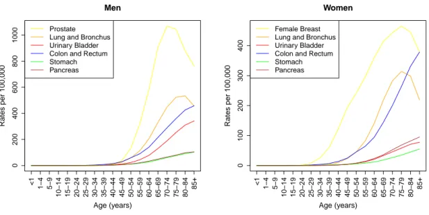
Figure 1.1: Age specific cancer incidence rates. The incidence of cancer grows steeply with increasing patient age. Data were obtained from the SEER Program of the US National Cancer Institute [1].
Among those barriers are both biological and biochemical defense mechanisms. Cells can be divided into stem cells and highly differentiated cells. The risk of DNA damage in the stem cells is minimized through two biological mechanisms: Stem cells divide only very rarely and the stem cell compartments protect them anatomically from external influences. The biochemical barriers include enzymes that destroy mutagens and DNA repair enzymes which find and repair structural changes in the DNA [76].
Epidemiologic studies, conducted e.g. by the US National Cancer Institute [1], showed that cancer incidence rates are highly age dependent. Figure 1.1 shows the age specific cancer incidence rates for American men and women for six different cancer sites.
Data were collected between 1992 and 2010. The plots show that for both men and women the risk for cancer incidence rises steeply with increasing age. These data confirm that many cancer types that are frequent in adults develop over years or decades leading to the relatively high age of cancer incidence [76].
During the past several decades extensive evidence has been found which documents the accumulation of increasing numbers of mutations in cells during their development from healthy to malign cells [29, 56, 76]. This means that many of the steps in tumor progression can be associated with the accumulation of genetic alterations in the cells’
genome. Colon cancer is very well studied because of the relatively good accessibility of the colonic epithelium. Therefore, the correlation between the accumulation of
mutations and an increasing malignancy of the cells has been studied most detailed for human colon carcinomas [29, 76].
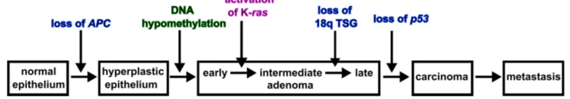
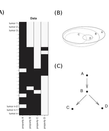
As illustrated in figure 1.2 colon cancer develops in several distinct steps. Each step can be linked to a genetic change in the corresponding cells on the way to increasing malignancy. However, only a small number of all colon cancer patients obtain the mutations in the order shown in figure 1.2 [76]. While in about 90 % of all colon carcinomas theAPC (adenomatous polyposis coli) gene on chromosome 5q is inactivated at a very early stage, only about 50 % have a K-ras mutation, show a loss of heterozygosity (LOH) on chromosome 17q involving p53 and an LOH on chromosome 18q [29, 74]. The specific gene which is affected on chromosome 18q is not yet identified with certainty. Promising candidates are the DCC (deleted in colorectal cancer) gene and the DPC4 (deleted in pancreatic cancer locus 4) gene [30, 62, 70].
Figure 1.2:Tumor suppressor genes and the progression of colon cancer. Identified tumor suppressor genes (TSGs) are the APC gene on chromosome 5q and p53 on chromosome 17p (blue). It is still unclear which TSG(s) are inactivated on chromosome 18q. About half of the colon carcinomas had a mutation on the K-ras gene (pink) and in most genomes of premalignant cells DNA hypomethylation had taken place (green). Figure reproduced from [76].
1.2 The hallmarks of cancer
In 2000 Hanahan and Weinberg [39] predicted that cancer research would develop into a logical science. This means that cancer could be explained by a small number of biological properties that are common to all cancer cells. The acquisition of such properties determines the development of cells into cancer cells. The authors suggest that these properties unbalance the cellular functions which are responsible for cell proliferation and homeostasis. They furthermore suggest, that all cancer-associated genes can be assigned to six alterations in cell physiology - the hallmarks - which all contribute to malignant growth:
1. Self-sufficiency in growth signals
Normal cells can only start to proliferate when they receive mitogenic growth signals. Otherwise they stay in a passive non-proliferative state. This is in con- trast to the behavior of tumor cells which are much less dependent on external growth signals. It has been shown for several human cancer types that tumor cells are able to synthesize stimulatory growth factors on their own [5, 36, 39]
which makes them much less dependent on their environment.
2. Insensitivity to antigrowth signals
In a healthy tissue, a cell can be kept in a quiescent state through antiprolif- erative signals. During the active proliferative phase healthy cells are receptive to signals from their environment and decide on the basis of these signals, if they go into a quiescent state (g0 phase) or if they grow (g1 and g2 phase).
Most antiproliferative signals are transmitted through the retinoblastoma pro- tein (pRb) pathway. If this pathway is disrupted, E2F transcription factors are liberated and thereby cell proliferation is allowed even in the presence of antigrowth factors.
3. Evasion of programmed cell death
The high cell proliferation rate is one of the main reasons for the enormous growth of tumor cell populations. But also the rate at which cell number de- creases plays a major role. Apoptosis, i.e. programmed cell death, is primarily responsible for this decrease. There is evidence, e.g. from studies in mouse models, that p53 plays an important role in the regulation of apoptosis which is in turn important barrier against tumor progression [14, 63, 67].
4. Limitless replicative potential
The three acquired biological properties of growth signal autonomy, insensitiv- ity to antigrowth signals and resistance to apoptosis allow cells to grow inde- pendently of external signals. It seems, however, that the acquisition of these properties is not sufficient to produce cells with unlimited growth. In addition to the signaling pathways between different cells, most cells have a specific in- tracellular program that controls their multiplication. When cells have divided for a certain number of times, they go into senescence, i.e. they stop dividing.
Tumor cells must find a way to circumvent these limitations in number. By studies on cultured human fibroblasts it could be demonstrated that disabling of the pRb and p53 TSGs allows cells to circumvent senescence and eventually achieve unlimited replicative potential [42].
5. Sustained angiogenesis
In order to ensure the unlimited multiplication of tumor cells they must be able to create an in vivo environment where they can grow. This ensures that a sufficient amount of oxygen and nutrients is provided for proper cell function and survival. An important element for the creation of such an environment is the formation of new blood vessels. Tumor cells initially have no ability to trigger angiogenesis. There is extensive evidence that tumors must acquire angiogenic abilities to ensure further tumor growth [16, 38].
6. Tissue invasion and metastasis
At some point during tumor development cells from the primary tumor go to adjacent tissues and eventually initialize the growth of a new tumor mass. The success of this new tumor colony depends of the presence of the other five acquired properties, as in the primary tumor. According to [65] it is not the enhanced cell proliferation rate, but rather tissue invasion and metastasis that are responsible for the many cancer deaths.
In 2011 Hanahan and Weinberg [40] further suggested that the acquisition of the six hallmarks is facilitated by two enabling characteristics:
1. Genome instability and mutation
In order to acquire the above described hallmarks several alterations in the tumor genome are necessary. Cancer cells often have increased mutation rates [55, 61]. These are achieved because cancer cells are more sensitive to DNA damaging agents, because of a malfunction of parts of the DNA repair ma- chinery, or both. The accumulation of mutations is additionally supported by damage in the systems that normally monitor genomic integrity. If the DNA can not be repaired these monitoring systems are responsible for killing cells with damaged DNA by triggering apoptosis or senescence, i.e. the cells cease to divide [43, 49, 64]. Genomic instability seems to be a property of the majority of human cancer cells. The defects in genome maintenance and repair must confer a selective advantage and thus support tumor progression, e.g. because they increase the mutation rates in premalignant cells [40].
2. Tumor-promoting inflammation
Almost every tumor tissue contains cells of the immune system and thereby shows inflammatory conditions as they normally occur in healthy tissues [28].
The immune system might try to destroy the tumor cells by means of these
immune responses. Hence, in order for the tumor to escape immune destruction it must acquire new mutations. It has been repeatedly demonstrated that inflammation has the undesired effect of promoting tumor progression and thus helps tumor cells to acquire hallmark capabilities [20, 23, 37, 40, 59].
Other properties of cancer cells have been proposed to be important for tumorigenesis and might therefore be added to the list of cancer hallmarks. The two most promising among those are:
1. Reprogramming energy metabolism
In order to maintain the enhanced proliferation in cancer cells their energy metabolism must be adjusted to ensure the cells’ supply with nutrients. Nor- mal cells produce their energy preferably through oxidative phosphorylation when aerobic conditions are given and only a small part of the cellular energy is obtained through the less effective glycolysis. Under anaerobic conditions the cells prefer energy production through glycolysis. Cancer cells are able to pro- duce their energy mostly by means of glycolysis also under aerobic conditions.
This state is termed “aerobic glycolysis”. The reason why cancer cells switch to glycolysis is still partly unclear. According to a hypothesis by Potter [57], which was refined by Vander Heiden et al. [71], increased glycolysis is important in the formation of new cells and therefore supports active cell proliferation.
2. Evading immune destruction
Research on immunodeficient mice suggests that the immune system plays an important role in preventing the formation of a tumor and its progression in non-virus induced cancer types [50, 69]. It could be observed that carcinogen- induced tumors grow more frequently and/or more rapidly in immunodeficient mice than in the immunocompetent controls. Similar results were obtained from transplantation experiments with mice. However, it is not yet clear to what extent antitumor immunity prevents the development of cancer in humans. In order to accept evading immune destruction as a core hallmark, more research will still be necessary [40].
Figure 1.3: Comparative genomic hybridization. Tumor and reference DNA are labeled green and red, respectively. The differentially labeled DNA is mixed and Cot-1 DNA is added. The mix is then hybridized to normal metaphase chromo- somes. Changes in copy number can be detected from shifts in the color, a shift to green means a gain, a shift to red represents a loss of chromosomes/chromosomal regions.
1.3 Comparative genomic hybridization
Comparative genomic hybridization (CGH) is a technique for the analysis of chromo- somes which was first reported by Kallioniemi et al. [48] in 1992 and shortly after by du Manoir et al. [27]. It allows to find changes in the copy number of chromosomes without growing cell cultures [77]. CGH makes it possible to compare tumor and normal DNA and to detect chromosomal regions of gain or loss of DNA sequences in the tumor genome. With the help of these results one may then study the identified DNA regions in more detail using other molecular biological techniques in order to detect possible oncogenes or TSGs [77].
A schematic overview of the CGH technique is given in figure 1.3. Tumor DNA and normal reference DNA are labeled with two different fluorochromes - the tumor DNA in green, the normal DNA in red. The DNA is then mixed in a 1:1 ratio and put on normal human metaphase preparations where they hybridize to target chromosomes.
A gain of chromosomal regions in the tumor DNA results in a higher green-to-red fluorescence ratio (> 1) in the concerned region, whereas a loss leads to a lower green-to-red ratio (< 1).
In their review, Weiss et al. [77] give a detailed description of the individual steps in- volved in the CGH technique and point out possible sources of error. After metaphase slides have been prepared and DNA has been isolated from the tissues, CGH involves the following steps:
1. DNA labeling
The tumor and reference DNA is labeled and cut by means of nick translation which is a molecular biological tagging technique. In nick translation single- stranded DNA fragments (“nicks”) are produced from the DNA with the help of DNase, a DNA degrading enzyme. Then DNA Polymerase I, an enzyme involved in DNA replication, is used to replace some of the nucleotides in the DNA with their labeled analogues [60]. In order to guarantee optimal hybridiza- tion, the fragment lengths of both test and reference DNA should be within the range of 500-1500 base pairs.
2. Blocking
In many chromosomal regions there are short repetitive DNA sequences. These are particularly numerous at the centromeres and telomeres and some specific chromosome regions. The presence of these sequences can cause that some gains and losses remain undetected thus resulting in a reduced amplitude of the green-to-red ratio. Therefore, unlabeled Cot-1 DNA, i.e. placental DNA which is enriched for repetitive DNA sequences, is used to block the repetitive DNA sequences.
3. Hybridization
For probe generation equal amounts of the labeled test and reference DNA are mixed and the Cot-1 DNA is added. Denaturation of the probe and the normal metaphase slides is done separately, then the probe is immediately added to the slides. The hybridization is left in a humid chamber at 40◦C for two to four days. After hybridization the slides are washed, dried and colored with a blue-fluorescent stain for chromosome identification.
4. Fluorescence Visualization and Imaging
Visualization of the green, red and blue fluorochromes is done using a fluores- cence microscope. After capturing the digital images of the fluorescent signals, for each chromosome the ratios of several high quality metaphases are averaged and plotted along ideograms of the corresponding chromosome. This generates a relative copy number karyotype which presents chromosomal areas of dele-
Figure 1.4: Relative copy number karyotype. The averaged green-to-red ratios are plotted against the chromosomal axis. Values greater than 1 represent a gain of chromosomal regions, values smaller than 1 stand for a loss.
tions or amplifications. An example is shown in figure 1.4. The ratio profiles can be interpreted in two ways using either fixed or statistical thresholds [77].
When using fixed thresholds, losses and gains are identified with the limits 0.75 and 1.25 or 0.85 and 1.15, while in the case of statistical thresholds the 95 % confidence interval (CI) limits of the ratio profile are taken. When using confidence intervals (CIs), gains or losses are present when the 95 % CI of the fluorescence ratio does not contain 1.0.
1.4 Tumor datasets
The performance of the methods developed in this thesis is verified using real tumor datasets. The same three datasets are used which were previously analyzed in [34]
in order to compare the performance of these methods to that of the maximum likelihood estimation (MLE) of the conjunctive Bayesian network (CBN) model. The data were generated with CGH and were obtained from the Progenetix database [8].
Progenetix is a molecular-cytogenetic database which collects previously published chromosomal aberration data. A descriptive analysis of the Progenetix data can be found in [7].
Renal cell carcinoma
The first dataset is on renal cell carcinoma (RCC). Parts of this dataset (251 cases) have been published before in [46]. The most frequent gains in this dataset are:
+5q(31) (25.2 %), +17q (21.2 %) and +7 (21.2 %). The most frequent losses are: –3p (59.4 %), –4q (29.9 %), –6q (25.5 %), –9p (24.4 %), –13q (23.1 %), –14q (17.9 %), –8p
(16.3 %) and –18q (14.7 %). As in [34] only the N = 12 copy number alterations (CNAs) used by Jiang et al. [46] are analyzed. They were selected using the method of Brodeur et al. [17], a statistical method to analyze structural aberrations in human cancer cells.
Among the CNAs listed above, the gain of chromosome 5p and the loss of 14q are not included. Instead, the gain of the Xp chromosome (9.6 %, often whole chromosome) is included as well as the gain of 17p (13.5 %). The dataset is reduced to theNP = 251 cases (patients) published in [46].
Breast cancer
The breast cancer (BC) dataset consists of 817 cases and 10 CNAs. The most frequent (> 20 %) gains are: +1(q31) (59.7 %), +8(q23) (48.0 %), +17q (36.2 %), +20(q) (31.7 %), +16(p) (25.1 %), +11q13 (24.5 %) and +3q (22.4 %). The most frequent losses (>20 %) are: –16(q) (29.0 %), –8p (27.8 %) and –13q (24.7 %) [34].
Colon cancer
The colorectal cancer (CRC) dataset consists of 570 cases and has 11 CNAs. The most frequent gains (> 20 %) in the CRC dataset are: +20(q13) (46.7 %), +13q (37.9 %), +8(q24), +7(q) (32.8 %) and +X(q24) (30.4 %). The most frequent losses are: –18(q22) (44.4 %), –8p(22) (34.2 %), –17p12 (25.3 %), –4(q) (23.3 %), –15q (19.2 %) and –1p (18.8 %) [34].
Each dataset is represented as a binary matrix D where rows are patients and columns are mutations or events. An element of the matrix is denoted as dji. Here, i ∈ {1, . . . , N} where N is the number of genomic events in the data and j ∈ {1, . . . , NP} where NP is the number of patients in the dataset. The j-th row in the matrix D is denoted as dj = (dj1, . . . , djN) and the i-th column is given by dTi = (d1i, . . . , dNPi)T.
The data D are noisy, it is observed with both systematic and random errors which can be ascribed to the sampling and measurement procedures [66]. There are several different sources for the systematic error. One source of error lies in the process of DNA extraction. During the extraction of DNA e.g. from cancer cells one may not always succeed in perfectly separating the tumor cells from the surrounding tissue.
Thus, the sample DNA might contain a small amount of DNA that actually comes
from healthy cells. Another possible source of error is intra-sample heterogeneity.
The progression of the disease might be different among the sample cells, therefore resulting in a homogeneous sample where not all cells have identical alterations. A further potential source of systematic error are repeated DNA sequences that occur at more than one location in the genome. The repeated sequences may cross-hybridize therefore making it impossible to assign the measurements always to the correct genomic region. The random errors are caused by different kinds of measurement errors which lie in the experimental procedure [66].
Methods
This chapter provides a description of the methods used throughout this thesis. Section 2.1 introduces some of the basic notations of graph theory and related terms which are used in the following sections. Section 2.2 explains the basics of conjunctive Bayesian networks (CBNs). Section 2.3 gives an introduction of support vector ma- chines (SVMs) and section 2.4 describes approximate Bayesian computation (ABC).
Both the SVM- and the ABC-based methods are combined with a number of search- ing algorithms which are discussed in section 2.5. The search is initialized using the heuristic approach of Jacob et al. [44] which is described in section 2.6.
2.1 Some basics of graph theory
The notations and definitions introduced in the following were taken from [26] and [35].
Graphs
A graph is a pair G= (V, E) of sets where E ⊆[V]2. The notation [V]2 means that the elements ofEare subsets ofV which consist of 2 elements. The elements ofV are called thevertices ornodes of the graph Gand the elements ofE are callededges.
When drawing a graph, a node is usually depicted as a dot or circle and an edge between two nodes is represented by a line.
Subgraphs
Consider the graphs G = (V, E) and G0 = (V0, E0). The graph G0 is said to be a subgraph of G, written asG0 ⊆G, if V0 ⊆V and E0 ⊆E.
Paths and cycles
A path is a non-empty graphP = (V, E) with nodes V ={v1, v2, . . . , vN} and edges E ={v1v2, v2v3, . . . , vN−1vN}with thevibeing all distinct. The pathP is also written asP =v1v2. . . vN.
Given a path P =v1v2. . . vN with N ≥ 3, a cycle is defined asC =P +vNv1. The cycleC can also be denoted as C =v1v2. . . vNv1.
Directed acyclic graphs
The graphs considered so far were undirected. Adirected graphG= (V, E) is a graph where every edge inE is an ordered pair of distinct nodes. When drawing a directed graph, an arrow normally marks the direction of an edge.
A directed acyclic graph (DAG) is a directed graph that does not contain cycles.
Adjacency matrix
The adjacency matrix A(G) = A of a graph G with N nodes is an N ×N-matrix where an off-diagonal element A(G)uv = Auv is equal to the number of edges from nodeu to node v, with u, v ∈V.
In this thesis only DAGs are considered. In this case, the matrixA(G) is binary and for all off-diagonal elements we have that Auv = 1 if there is a directed edge from u to v, and Auv = 0 otherwise. Because there are no loops in DAGs, all the diagonal elements of A are zero.
Note that the adjacency matrix of a directed graph is not symmetric.
Transitive reduction
Following Aho et al. [3], the transitive reduction of a DAGG is defined as a smallest subgraph ofG which contains a path from node u to node v whenever G contains a path fromu tov. In other words, a DAG Gt is said to be a transitive reduction of G provided that
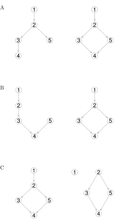
Figure 2.1: Transitive graph and transitive reduction. (A) Transitive graph. (B) Transitive reduction of the graph shown in (A).
(i) Gt has a directed path from node u to node v if and only if G has a directed path from node u to nodev, and
(ii) there is no graph with fewer edges thanGt satisfying condition (i) [3].
Figure 2.1 (A) displays a transitive graph, the corresponding transitive reduction is shown in figure 2.1 (B). The transitive reduction of a finite DAG Gis unique and is always a subgraph of G.
Intermediate states
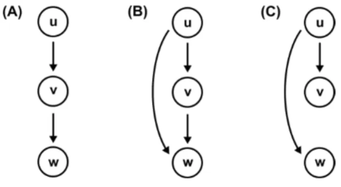
An edge uw in a graph G is called a single intermediate state if there is exactly one nodev, v ∈V \ {u, w}, for which in the adjacency matrix of the graph we have that Auv = 1 and Avw = 1. To illustrate the single intermediate states, figure 2.2 (A) shows a subgraph of a graph Gcontaining the nodes u, v and w.
An edge uw in a graph G is called a multiple intermediate state if there are two or more nodesvi, vi ∈V \ {u, w}, i∈ {1, . . . , N −2}, for which in the adjacency matrix we have that Auvi = 1 and Aviw = 1. Figure 2.2 (B) gives an example of a multiple intermediate state. It shows a subgraph of a graph G that contains the nodes u, v1, v2 and w.
Figure 2.2:Intermediate states. (A) Single intermediate state. There is only one node,v, for which Auv = 1 and Avw = 1. (B) Multiple intermediate state. There are two (or more) nodes,v1 andv2, for which Auvi = 1 and Aviw = 1.
2.2 Conjunctive Bayesian networks
The most common way for learning the parameters of a statistical model is by analyz- ing the likelihood function. The optimal parameters for describing a specific dataset are found through maximization of the likelihood function. For models where the maximization can not be done in closed-form, parameter fitting is done via maxi- mum likelihood estimation (MLE).
An example for such a model are the conjunctive Bayesian networks (CBNs) [11–
13, 34]. Conjunctive Bayesian networks (CBNs) are probabilistic graphical models that can be used for describing the accumulation of events, e.g. genomic events. A CBN model is a specialization of a Bayesian network where an event can only occur if all of its parents have already occurred. CBNs are also a generalization of tree models [24, 25, 46, 75]. In contrast to oncogenetic tree models they allow for an event to depend on more than one predecessor event. Therefore, CBNs allow for an arbitrary partial order on the events which makes them able to model a larger range of biomedical problems than oncogenetic tree models.
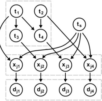
A CBN can be used to model the accumulation of mutations in a tumor. CBNs assume that tumors progress along a transitively reduced DAG, where each node corresponds to a mutation event and parent nodes are mutations that typically pre- cede a child mutation. CBNs are Bayesian networks that account for the variability and stochasticity of the timing of mutation events as well as of observation times. A graph of a CBN example is shown in figure 2.3. With every mutation i a random variable ti, i ∈ {1, . . . , N} = [N] is associated which is the time it takes for the
Figure 2.3: Graph of a CBN example. The CBN in the upper left part of the image shows the waiting timesti of mutations i= 1, . . . ,4 and the order in which the mutations occur: mutations 1 and 2 can occur independently; mutation 3 can only occur after mutation 1 occurred, t1 < t3, and the presence of mutation 4 is conditional on mutations 1 and 2 being present, i.e. t1, t2 < t4. The observation time ts is depicted in the upper right part of the image - it is independent of the waiting times ti. A mutation i is present in the genotype xj = (xj1, . . . , xj4) of a patientjifti < ts. The observationsdj = (dj1, . . . , dj4) contain errors which occur independently for each mutation with probability. Figure reproduced from [34].
respective mutation to develop. Here, N is the total number of possible mutations.
The set of parent mutations pa(i) is defined as the set of mutations that need to be present before a specific mutation i can occur. The waiting times ti are defined to be exponentially distributed with parameter λi given that all parent mutations pa(i) are present:
ti ∼ E(λi) + max
j∈pa(i)tj. (2.1)
The parameter λi > 0 is the parameter of the exponential distribution, often called the rate parameter.
The upper left part of figure 2.3 shows the waiting timesti of mutations i= 1, . . . ,4 and the order in which the mutations occur. Mutations 1 and 2 can occur inde- pendently, mutation 3 can only occur after mutation 1 occurred, i.e. t1 < t3, and the occurrence of mutation 4 is conditional on mutations 1 and 2 being present, i.e.
t1, t2 < t4.
CBNs furthermore include a time of diagnosistsfor the tumor of each patientj which models the overall progression of that tumor. The timets which is independent of the waiting timestiis shown in the upper right part of figure 2.3. The time of diagnosis is sampled from an exponential distributionts ∼ E(λs) for each patient. Since the entire parameter vector λ = (λ1, . . . , λN, λs) is not likelihood identified, the parameter λs for the observation time is set to 1.
The perfect data without observational errors are represented as a binary matrix X = (xji), where i ∈ {1, . . . , N} and j ∈ {1, . . . , NP}. Mutation i is present in patient j at diagnosis, i.e. xji = 1 if ti < ts, otherwise xji = 0. The genotype of a patient j is denoted as xj = (xj1, . . . , xjN) and is formed by the j-th row in the matrix X. The i-th column of X is denoted asxTi = (x1i, . . . , xNPi)T.
As introduced in section 1.4, the actual observations are denoted as D = (dji) and may differ from the perfect dataX due to observational errors which are assumed to occur independently for each mutation with probability. Both the perfect genotype xj and the observed genotype dj of a patientj are shown in the lower part of figure 2.3.
Parameter estimation
For a given network G the log-likelihood of NP independent observations (patients) D= (d1, . . . ,dNP) is [34]
`D(,λ, G) =
NP
X
j=1
log
X
xl∈J(G)
Prob[dj|xl] Probλ,G[xl]
. (2.2)
The formula for the log-likelihood is composed by
• the prior probability that the genotypexl occurs Probλ,G[xl] = Probλ,G
i:xmaxli=1ti < ts< min
j:xlj=0tj
,
• the conditional probability of an observationdj given genotypexl
Prob[dj|xl] =d(xl,dj)(1−)n−d(xl,dj),
• the sum Pxl∈J(G) where J(G) is the lattice of order ideals, containing all geno- typesxl compatible with the graph G (see [13]), and
• the sumPNj=1P over all NP observations in D.
For a fixed network G the parameters and λ are estimated in a nested expecta- tion–maximization (EM)-algorithm which consists of two loops. In the inner loop the estimate of the noise level ˆ is obtained which locally maximizes `D(,λˆ(k), G) for a given ˆλ(k) estimated at the previous iteration and a given network G from the previous step of the simulated annealing (SA) procedure. The value ˆis then used in the outer loop to find the estimator ˆλ. Here, k is the index of the outer loop.
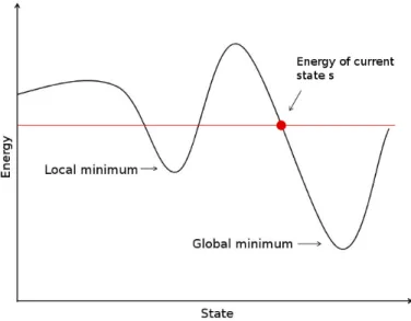
In order to actually learn a network structure G from a given dataset D, the EM- algorithm is embedded into a simulated annealing (SA) procedure for performing the search in the graph space. During this, one first computes the log-likelihood
`D(ˆ,λ, G) for a givenˆ G and D. Then a new networkG0 is generated randomly and is accepted if either `D(ˆ,λ, Gˆ 0) > `D(ˆ,λ, G) or, alternatively it is accepted with aˆ probability exp(−[`D(ˆ,λ, G)ˆ −`D(ˆ,λ, Gˆ 0)]/T). During the process the annealing temperature T tends to zero and the probability to accept changes that decrease the log-likelihood also does.
The following two paragraphs describe how the proposal of a new graph topology is performed in the software package ct-cbn, version 0.1.04 (Oct 2011), available on the website http://www.bsse.ethz.ch/cbg/software/ct-cbn.
Compatibility
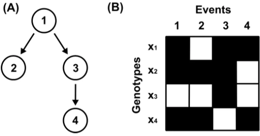
Consider the graph G depicted in figure 2.4 (A) and the dataset D shown in figure 2.4 (B). The example dataset consists of four genotypes and four mutations, where the rows represent the genotypes and the columns correspond to the mutations. In the figure, events that are present in a patient’s genotype, i.e. xji = 1, are marked by black fields. White fields denote absent events. A genotype xj of a patient j is called compatible with the graph G if for every event that is present in xj all parent mutations are also present. Genotypex1 is compatible with the graph because the condition is fulfilled for all three events that are present. Event x11 can occur independently of any parent node,x13can occur because its parentx11is present, and the occurrence of eventx14is conditioned on the presence ofx13. Genotypex2 is also compatible with the graph Gdue to similar reasons. Genotype x3 is not compatible because here only event x33 is present, but its parent x31 is not. Genotype x4 is not compatible either. Here, the occurrence of events x41 and x42 is in agreement with the graph, x41may occur independently because it has no parent events andx42
Figure 2.4: Example graph and dataset. (A) Example graph with four nodes.
(B) Example dataset where every row represents a genotype and the columns cor- respond to the events. Black fields mark events that are present, absent events are shown in white.
can occur because its parent x41 is also present. However, the presence of event x44 without event x43 having occurred is not in agreement with the graph and therefore this genotype is not compatible with the graph.
More formally this means that a genotype xj is not compatible with a graph G if for any edge ik in the graph we have that xji = 0 and xjk = 1 for at least one pair i, k∈1, . . . , N.
For a dataset D that consists of NP patients (or genotypes) and N events one can then calculate a measure α for the compatibility of the dataset with a graph G
α=Nc/NP, (2.3)
whereNcis the number of genotypes inD that are compatible with the graphGand 0< α < 1. The value α can be interpreted as the proportion of genotypes that are compatible withG among all genotypes in D.
Proposal of a new graph topology
During each step of the simulated annealing (SA) a new graph G0 is proposed with one edge difference to the previous graph G. To obtain G0, a pair of numbers u, w is drawn uniformly from {1, . . . , N} with u 6= w and the respective entry A0uw in the adjacency matrix of G0 is flipped, from 0 to 1 or vice versa. The graph is then transitively reduced. To assess the quality of the new graph, the compatibilityα0 of the dataset D with the graph G0 is calculated according to eqn. (2.3).
Figure 2.5: Edge replacement. (A) Original edge constellation in graphG with edgesuvand vw. (B) Proposed edgeuw is a transitive edge. (C) In the new graph G0 the edge uw is kept and instead the edgevw is removed.
If in the new graph we have that A0uw = 1, then an edge was added. If the graph contains a cycle or if the edgeuwis a multiple intermediate state (see p. 23),α0 is set to 0. If the edge uwis a single intermediate state (see p. 23), an edge replacement is made as shown in figure 2.5. The original edge constellation in graphGwith edgesuv andvwis shown in figure 2.5 (A). The edgeuwwould introduce a single intermediate state as illustrated in figure 2.5 (B). In this case, the edgeuwis kept in the new graph G0 and instead the edge vw is removed, as shown in figure 2.5 (C).
The compatibility α of the dataset D with the graph G is also computed following eqn. (2.3). α0 > α means that the proportion of genotypes inD compatible with the graph is higher in the case ofG0 compared toG. In this case the graphG0 is accepted as a candidate graph. If α0 < α, the graph G0 is accepted as a candidate graph with probability exp [(α0−α)/0.05].
For the accepted candidate graph the likelihood `D(ˆ,λ, Gˆ 0) is then calculated.
2.3 Support vector machines
Support vector machines (SVMs) [15, 21, 22, 72] belong to a class of supervised learning algorithms which can be used for classification and regression. When doing two-class classification an SVM takes a set of n-dimensional training samples with known class membership as input, wherenis the number of attributes in each sample.
The aim of the SVM is to find an (n-1)-dimensional hyperplane that separates the data best into the two classes.
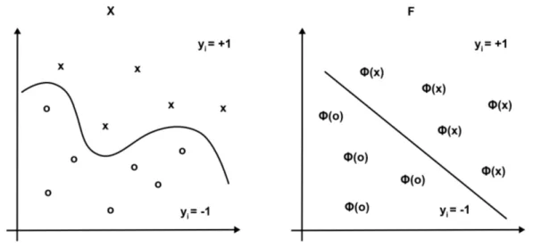
In the following section the key properties of SVMs are explained for the case of linearly separable data. In the case of real world data the separation of the data is normally not possible without error. A modification of SVMs that accounts for this case is introduced in section 2.3.2. If the data can not be separated linearly it can be mapped to a feature space where linear separation is again possible. The explicit mapping of the data can be avoided by using the kernel-trick. This is explained in section 2.3.3.
2.3.1 Linearly separable data
The input to the training algorithm, the training data, is a set of training samples which is usually denoted by
Dtrain = ((x1, y1), . . . ,(xl, yl)). (2.4)
The xi, xi ∈ X, are called the samples, where i = 1, . . . , l and l is the number of samples. X ⊆Rn is called the input space. The yi ∈ {−1,1} are the according class labels.
If the dataset is linearly separable, a hyperplane h ∈ Rn−1 exists which divides the data correctly into its two classes. This splits the space into a positive and a negative halfspace. The hyperplane’s normal vector w points by definition into the positive halfspace which contains class +1. The aim is to find the hyperplane with the maximal margin to the nearest data points of each class - the maximum-margin hyperplane. The nearest data points are called thesupport vectors.
Figure 2.6 shows an example dataset where the data from class -1 are marked in green and the data in class +1 are shown in red. The two boundary hyperplanes through the nearest data points x+ and x−, drawn as dashed lines, are chosen such that the geometric marginγ between them is maximized.
Any hyperplane hcan be written as the set of points xh satisfying
hw·xhi+b = 0, (2.5)
where w is the hyperplane’s normal vector, b is a constant which determines the distance of the hyperplane to the origin of the coordinate system andhw·xhi is the dot product between the two n-dimensional vectors w and xh.
Figure 2.6: Optimal hyperplane. An example dataset is shown with data from class -1 marked in green and data from class +1 shown in red. The two dashed lines are the boundary hyperplanes through the nearest data points x+ and x−. They are chosen such that the geometric margin γ between them is maximized. The optimal hyperplanehlies exactly in between those two hyperplanes and separates the data perfectly into the two classes.
Having a solution for the optimal hyperplane h we can formulate the decision as f(x) = sgn(hw·xi+b) primal form (2.6) f(x) = sgn
l
X
i=1
αiyihxi·xi+b
!
dual form, (2.7)
where xis a test sample.
The optimal hyperplane h lies exactly in between the boundary hyperplanes and separates the data perfectly into the two classes. The geometric marginγ is invariant to rescalings of w and b. Therefore, w and b can be rescaled such that the two boundary hyperplanes through the nearest points x+ and x− are described by
hw·x+i+b = 1 and hw·x−i+b=−1. (2.8)
Using geometry, the margin between these two hyperplanes can be calculated as 2 kwk. This means that the maximal margin of the hyperplanehcan be found by minimizing kwk. The expression kwk denotes the norm of the vector w.
Solving the optimization problem described above is difficult because the norm of w involves a square root. One can substitute kwk with 12kwk2 without changing the
solution. This results in a quadratic programming optimization problem:
min(w,b)
1
2kwk2 (2.9)
subject to
yi(hw·xii+b)≥1 for any i= 1, . . . , l. (2.10) The equality sign in eqn. (2.10) holds for the support vectors, the inequality holds for all the other samples xi in the training dataset.
The solutions of (2.9) are obtained using a Lagrangian approach. The primal La- grangian is given by
L(w, b,α) = 1
2kwk2 −
l
X
i=1
αi[yi(hw·xii+b)−1], (2.11) with Lagrange multipliersαi ≥ 0. The optimal solutions are denoted by w∗, b∗ and α∗i. For non-zeroα∗i the Karush-Kuhn-Tucker complementarity condition
αi∗[yi(hw∗·xii+b∗)−1] = 0 (2.12) is only fulfilled by the support vectors. For all the other vectorsxi the α∗i are 0.
In order to obtain the dual Lagrangian L is minimized with respect to w and b.
Hence, setting
∂
∂bL(w, b,α) = 0 and ∂
∂wL(w, b,α) = 0 (2.13) yields
l
X
i=1
αiyi = 0 and w=
l
X
i=1
αiyixi. (2.14)
Note that w is a linear combination of the training vectors as can be seen in eqn.
(2.14). The constantb is obtained by b = 1
r
r
X
k=1
yk− hx·xki, (2.15)
where k = 1, . . . , r are the indices of the support vectors and r is the number of support vectors.
Substituting the conditions (2.14) into the primal form of the Lagrangian (2.11) leads
to the dual form of the Lagrangian L(α) =
l
X
i=1
αi−1 2
l
X
i,j=1
αiαjyiyjhxi·xji. (2.16) Hence the optimization problem can be expressed as
max
(α) l
X
i=1
αi− 1 2
l
X
i,j=1
αiαjyiyjhxi·xji (2.17) subject to
l
X
i=1
yiαi = 0 and αi ≥0, i= 1, . . . , l (2.18) which is easier to solve than the problem in the primal form (equations (2.9) and (2.11)) because the constraints are less complex than those in eqn. (2.10).
2.3.2 Soft margin SVM
In practice, the training dataset will contain errors e.g. due to noise so that an optimal separation of the data with a linear SVM will not be possible. Therefore, Cortes and Vapnik [21] introduced a modification of the SVM algorithm. For each training vector xi aslack variable ξi ≥0 is introduced which measures the degree of misclassification of the data xi:
yi(hw·xii+b)≥1−ξi, i= 1, . . . , l. (2.19)
The soft margin SVM is illustrated in figure 2.7. In the example dataset the data from class -1 are shown as green dots, the data in class +1 are drawn in red. The dashed lines are the two boundary hyperplanes, the solid line is the optimal hyperplane h.
The green and red dots in between the two boundary hyperplanes are noisy data points that cannot be classified correctly.
Of course one can always fulfill the constraint in eqn. (2.19) by making the ξi large enough. This trivial solution is to be prevented by introducing a function which penalizes non-zero ξi. Then the optimization problem becomes
min
(w,ξ,b)
( 1
2kwk2+C
l
X
i=1
ξi
)
(2.20)