On the Approximation of Rough Functions with Artificial Neural Networks

(1)

Research Collection

Master Thesis

On the Approximation of Rough Functions with Artificial Neural Networks

Author(s):

De Ryck, Tim Publication Date:

2020-01-31 Permanent Link:

https://doi.org/10.3929/ethz-b-000397533

Rights / License:

In Copyright - Non-Commercial Use Permitted

This page was generated automatically upon download from the ETH Zurich Research Collection. For more information please consult the Terms of use.

ETH Library

(2)

On the Approximation of Rough Functions with Artificial Neural

Networks

Master’s Thesis Tim De Ryck

Friday 31

^st

January, 2020

Advisor: Prof. Dr. Siddhartha Mishra Department of Mathematics, ETH Z¨urich

(3)

(4)

Deep neural networks and the ENO procedure are both efficient frameworks for approximating rough functions. We prove that at any order, the stencil shifts of the ENO and ENO-SR interpolation procedures can be exactly obtained using a deep ReLU neural network. In addition, we construct and provide error bounds for ReLU neural networks that directly approximate the output of the ENO and ENO- SR interpolation procedures. This surprising fact enables the transfer of several desirable properties of the ENO procedure to deep neural networks, including its high-order accuracy at approximating Lipschitz functions. Numerical tests for the resulting neural networks show excellent performance for interpolating rough functions, data compression and approximating solutions of nonlinear conservation laws.

(5)

(6)

In the first place, I would like to thank my supervisor Prof. Dr. Siddhartha Mishra.

He suggested a topic that seamlessly combines two of my research interests, numerical mathematics and deep learning. This, together with his excellent guidance, made it a pleasure to develop this thesis. In particular, I thank him for providing me with a workplace at SAM and for giving me the chance to work on a research paper.

Second, I owe thanks to Dr. Deep Ray for the pleasant collaboration on this topic. It is his research findings that constitute the foundation of this thesis. I am particularly grateful to him for letting me use his code and for the fruitful discussion on ENO regression networks.

Finally, I am thankful for my parents and the opportunities they provided. My time in Z¨urich has been a great experience and it would not have been possible without their support.

(7)

(8)

Contents v

1 Introduction 1

2 Preliminaries 5

2.1 Feedforward artificial neural networks . . . 5

2.2 Basic ReLU calculus . . . 7

3 Function approximation with neural networks 11 3.1 Expressive power of neural networks . . . 11

3.2 Approximation of Lipschitz continuous functions by deep ReLU networks 14 3.2.1 Approximation with continuous weight assignment . . . 15

3.2.2 Approximation with discontinuous weight assignment . . . 16

4 ENO interpolation with ReLU neural networks 21 4.1 ENO interpolation . . . 21

4.2 ENO reconstruction . . . 24

4.3 ENO stencil selection with ReLU neural networks . . . 26

4.4 ENO interpolation with ReLU neural networks . . . 31

5 Second-order ENO-SR interpolation with ReLU neural networks 37 5.1 Second-order ENO-SR interpolation . . . 37

5.1.1 Algorithm . . . 37

5.1.2 Properties . . . 39

5.1.3 ENO-SR-2 stencil selection with ReLU neural networks . . . 40

5.2 Adapted second-order ENO-SR interpolation . . . 45

5.2.1 Algorithm . . . 45

5.2.2 Properties . . . 46

5.2.3 Adapted ENO-SR-2 stencil selection with ReLU neural networks 49 5.2.4 Adapted ENO-SR-2 interpolation with ReLU neural networks . . 50

6 Numerical results 59 6.1 Training procedure . . . 59

6.1.1 Training data sets . . . 60

6.1.2 Training details . . . 61

(9)

Contents

6.2 Performance of DeLENO(-SR) methods . . . 63

6.2.1 DeLENO classification networks . . . 63

6.2.2 DeLENO regression networks . . . 64

6.2.3 DeLENO-SR classification network . . . 68

6.2.4 DeLENO-SR regression network . . . 69

6.3 Applications . . . 70

6.3.1 Function approximation . . . 70

6.3.2 Data compression . . . 70

6.3.3 Conservation laws . . . 75

7 Conclusion 79

A Weights and biases for trained networks 81

B Multi-resolution representation of functions for data compression 83

Bibliography 85

vi

(10)

Introduction

Functions of limited regularity arise in a wide variety of problems in mathematics, physics and engineering. Weak solutions of nonlinear partial differential equations constitute a prominent class of such rough functions. For instance, solutions of Hamilton- Jacobi equations and other fully nonlinear PDEs are in general only Lipschitz continuous [Evans, 1998]. Discontinuous functions appear as solutions of nonlinear hyperbolic systems of conservation laws, e.g. the compressible Euler equations of gas dynamics, as they can contain shock waves [Dafermos, 2010]. Similarly, solutions to the incom- pressible Euler equations would well be only H¨older continuous in the turbulent regime [Eyink and Sreenivasan, 2006]. Another notable class of rough functions are images.

On account of their sharp edges, they are usually assumed to be no more than functions of bounded variation.

In view of their prevalence, the need for numerical procedures that can efficiently and robustly approximate rough functions can not be undervalued. However, in classical approximation theory the accuracy of the interpolant usually relies on the regularity of the underlying function in a critical way. This poses a severe problem for the interpolation (or approximation) of rough functions. For continuous, piecewise smooth functions, standard linear interpolation procedures are only first-order accurate [Ar`andiga et al., 2005] and the order of accuracy (in terms of the interpolation mesh width) degrades even further if the underlying function is discontinuous. Apart from a reduced accuracy, classical approximation procedures can also cause the emer- gence of spurious oscillations near jump discontinuities. This issue particularly arises when dealing with solutions of nonlinear hyperbolic systems of conservation laws that contain shock waves. The approximation of rough functions clearly poses a formidable challenge.

In Chapter 2 of this thesis, we present the concept of artificial neural networks. In- spired by the neural circuits in the human brain, they are formed by concatenating affine transformations with pointwise application of nonlinearities, the so-called activation functions. Being only piecewise smooth themselves, interpolation using neural networks will lead to significantly different results than the polynomial approximations arising from classical interpolation theory. The expressiveness of neural networks man- ifests itself through the universal approximation properties the networks possess, as will be discussed in Chapter 3. In particular, they can approximate piecewise smooth functions with an arbitrary degree of accuracy. These universality results however do

(11)

1. Introduction

not specify the precise architecture of the approximating network. This changed re- cently, when for example [Yarotsky, 2017] was able to explicitly construct deep neural networks with ReLU activation functions that can approximate Lipschitz functions to second-order accuracy. Moreover, [Yarotsky and Zhevnerchuk, 2019] were able to construct deep neural networks with alternating ReLU and sine activation functions that can approximate Lipschitz (or H¨older continuous) functions to exponential accuracy.

In both cases, very precise estimates on the type and architecture of the underlying networks were given. These results give insight in how artificial neural networks can be used to construct approximation of rough functions and are therefore a starting point for this thesis.

Although the importance of the results of Yarotsky is well established, as they illustrate the power of deep neural networks in approximating rough functions, there is a practical issue in the use of these deep neural networks we want to address. The neural networks constructed in [Yarotsky, 2017] are mappingsfN from the space coordinatex∈D⊂R^d to the outputf_N(x)∈R, with as goal to approximate an underlying functionf :D→R. Hence, for every given function f, a new neural network f_N has to be obtained. This happens through the minimization of a loss function with respect to a finite set of samples of f [Goodfellow et al., 2016]. Although it makes sense to train networks for each individual functionf in high dimensions, for instance in the context of uncertainty quantification of PDEs [Lye et al., 2019], doing so for every low-dimensional function is unrealistic as this minimization procedure is computationally far more expensive than classical interpolation procedures. This problem can be resolved by noting that in a large numbers of contexts, the goal of approximating a function f is in fact finding a mapping {f(xi)}ⁱ 7→ If, where {f(xi)}ⁱ is a vector containing the function values of f at some sampling points and where the interpolant If approximates f. Hence, one would like to construct neural networks that map the input vector to an output interpolant (or its evaluation at certain sampling points). It is unclear if the networks proposed by Yarotsky can be adapted to this setting.

Another (a priori very different) way to interpolate rough functions with a high accuracy is the use of data dependent interpolation procedures, a renowned example being the essentially non-oscillatory (ENO) procedure, which we will introduce in Chapter 4. It was first developed in the context of the reconstruction of non-oscillatory polynomials from cell averages and has proven its value in high-order accurate finite volume schemes for the approximation of the solutions of hyperbolic PDEs [Harten et al., 1987].

Moreover, ENO was shown to satisfy a subtle non-linear stability property, the so-called sign property[Fjordholm et al., 2013]. Later, ENO was adapted for interpolating rough functions [Shu and Osher, 1989]. Once augmented with a sub-cell resolution (SR) procedure of [Harten, 1989], which will be introduced in Chapter 5, it was provided in [Ar`andiga et al., 2005] that the ENO-SR interpolant also approximated (univariate) Lipschitz functions to second-order accuracy. On account of their desirable properties, the ENO and ENO-SR interpolation procedures have also been successfully employed in the numerical approximation of Hamilton-Jacobi equations [Shu and Osher, 1991] and in data compression in image processing [Harten et al., 1997, Ar`andiga et al., 2005].

As both deep neural networks and the ENO procedure provide frameworks for the efficient approximation of rough functions, it is natural to explore links between these two a priori disconnected concepts. The main goal of this thesis is to shed light on these 2

(12)

interpreted as a classification or a regression problem. We prove that for any order, the ENO interpolation procedure can be cast as a suitable deep ReLU neural network in the classification context. When interpreted as a regression problem, we prove the existence of a deep ReLU neural network that approximates the ENO interpolation procedure without being deprived of some of ENO’s desirable properties. In Chapter 5, we propose a new variant of the piecewise linear ENO-SR procedure of [Harten, 1989] and prove again that it can be cast as a deep ReLU neural network in the classification context.

In addition, we prove that there exists a deep ReLU neural network that provides an approximation of a piecewise smooth function that is second-order accurate, up to an arbitrarily small constant error.

In Chapter 6, we investigate whether it is possible to (re)obtain (ortrain) ReLU neural networks that satisfy the accuracy results of Chapter 4 and Chapter 5 based on a so- called training data set. This data set contains vectors of function evaluations on a grid and their corresponding ENO(-SR) interpolants. We describe in detail how to generate these data sets and how to train networks to obtain what we term as DeLENO (Deep Learning ENO) approximation procedures for rough functions. Furthermore, we test the performance of these newly proposed DeLENO procedures in different contexts and explore the effect of input scaling on the performance. To stress their practicality, we conclude the thesis by showing how the DeLENO interpolation procedures can be applied for function approximation, data compression and the approximation of solutions of conservation laws.

(13)

(14)

Preliminaries

In statistics, machine learning, numerical mathematics and many other scientific disci- plines, the goal of a certain task can often be reduced to the following. We consider a (usually unknown) function f :D⊂R^m → Rⁿ and we assume access to a (finite) set of labelled data S ⊂ {(X, f(X)) : X ∈ D}, using which we wish to select an approximation ˆf from a parametrized function class {f^θ :θ ∈ Θ} that predicts the outputs of f on D with a high degree of accuracy. Classical choices include affine functions (linear regression), splines and many others. In the past decade, the use of artificial neural networks has gained popularity. In the following section, this class of functions is introduced, with special attention for ReLU deep neural networks, as these will form the cornerstone of this thesis. Afterwards, we present some very basic properties of ReLU neural networks.

2.1 Feedforward artificial neural networks

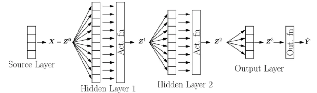
Artificial neural networks (ANNs) can be divided into many different categories. One of the most straightforward network types is the multilayer perceptron (MLP) or feedforward artificial neural network. These models are called feedforward because of the absence of feedback connections. Artificial neural networks that do have such connections are called recurrent neural networks. In feedforward artificial neural networks, a feedforward structure is created by stacking neurons, which are the basic computing units, in multiple layers. The input is fed into the source layer and flows through a number ofhidden layers to theoutput layer. An example of an MLP with two hidden layers is shown in Figure 2.1.

In the following, we formalize the definition of a feedforward artificial neural network.

Definition 2.1 Let L, n₀, n₁, . . . , n_L ∈N with L>2, let W^l ∈Rⁿ^l^×n^l−1 and b^l ∈Rⁿ^l for l = 1,2. . . , L. Let A^l be the affine linear map given by A^l : Rⁿ^l−1 → Rⁿ^l : x 7→

W^lx +b^l and let ρ^l : Rⁿ^l → Rⁿ^l be a function, for each l = 1,2. . . , L. A map Φ :Rⁿ⁰ →Rⁿ^L defined by

Φ(x) = (ρ^L◦ A^L◦ρ^L−1◦ · · · ◦ρ¹◦ A¹)(x) (2.1) for allx∈Rⁿ⁰ is called a feedforward artificial neural network of depthL. The network is said to have depthL, widthmaxini and activation functionsρ¹, . . . , ρ^L. Furthermore, W¹, . . . , W^L and b¹, . . . , b^L are called the weights and biases of the network.

(15)

2. Preliminaries

X=Z⁰ Z¹ Z² Z³

Act.fn Act.fn Out.fn

Yˆ

Source Layer

Hidden Layer 1 Hidden Layer 2

Output Layer

Figure 2.1: An MLP with 2 hidden layers. The source layer transmits the signalX to the first hidden layer.

The final output of the network isYˆ.

In this terminology, a feedforward ANN of depth L consists of an input layer, L−1 hidden layers and an output layer. It is said to be deep if L>3, in this case we speak of a feedforward deep neural network (DNN). We denote the vector fed into the input layer byZ⁰. Thel-th layer (withn_l neurons) receives an input vectorZ^l−1 ∈Rⁿ^l−1 and transforms it into the vectorZ^l ∈Rⁿ^lby first applying the affine linear transformation, followed by the activation functionρ^l,

Z^l=ρ^l(W^lZ^l−1+b^l), 16l6L, (2.2) withZ^l serving as the input for the (l+ 1)-th layer. Note that it is only interesting to choose nonlinear activation functions; if all activation functions are linear, the network reduces to an affine linear map. Many suitable options remain, common choices being (the multidimensional version of) the standard logistic function, the hyperbolic tangent and the rectified linear unit (ReLU). This last function is defined as

ReLU :R→R:x7→max{x,0}= (x)₊, (2.3) and has grown over the past year to the activation function of choice in many applications. Thanks to its simple form and its even simpler derivative, it is computationally cheaper to optimize a network with ReLU activation functions than a network with for instance sigmoidal activation functions. ReLU neural networks also partly resolve the saturation problem that is typical for the sigmoidal function: whereas the derivative of a sigmoidal function vanishes for both large positive and large negative values, the derivative of the rectified linear unit only vanishes for negative values. This facilitates again the problem of finding the optimal network, as most optimization algorithms fundamentally depend on the gradient to find an optimum. Furthermore, ReLU neural networks are also able to exactly represent some very basic, but useful functions. This is the topic of Section 2.2. This also allows the construction of explicit approximations of continuous functions, as will be seen in Chapter 3. It is the combination of these theoretical properties and its computational efficiency that makes the ReLU neural network ubiquitous nowadays. As we will almost exclusively use this type of multilayer perceptron in this thesis, we formalize the concept of an ANN that uses the rectified linear unit as activation function.

Definition 2.2 Let L, n0, n1, . . . , nL ∈ N with L > 2. For l = 1,2. . . , L −1, let ρ^l :Rⁿ^l →Rⁿ^l be a function that satisfies ρ^l(x) = (ReLU(x1), . . . ,ReLU(xnl))^T for all x ∈ Rⁿ^l and let ρ^L : Rⁿ^L → Rⁿ^L satisfy ρ^L(x) = x for all x ∈ Rⁿ^L. A feedforward 6

(16)

artificial neural network of depthLwith activation functionsρ¹, . . . , ρ^Lis called a ReLU neural network of depth L.

Definition 2.3 Let L, n0, nL∈N with L >2. Then we denote by N_L,n₀_,n_L the set of ReLU neural networks that have depth L, input dimension n₀ and output dimension nL.

We can now also make the connection with the problem setting in the introduction of this chapter. The function class under consideration in this case, is of course those of feedforward artificial neural networks. For consistency, we setn0 =mandnL=n. The parameter space Θ then consists of the weights and biases of the network. Depending on the nature of the problem, the output of the ANN may have to pass through an output functionS to convert the signal into a meaningful form. In classification problems, a suitable choice for such an output function would be thesoftmax function

S(x) :Rⁿ→Rⁿ:x7→ e^x¹ Pn

j=1e^x^j, . . . , e^xⁿ Pn

j=1e^x^j

!

. (2.4)

This choice ensures that the final output vector ˆY =S(Z^L) satisfiesPn

j=1Yˆj = 1 and 0 6 Yˆj 6 1 for all 1 6 j 6 n, which allows ˆYj to be viewed as the probability that the inputZ⁰ belongs to thej-th class. Note that the class predicted by the network is arg max_jYˆ_j. More output functions, and more information on multilayer perceptrons in general, can be found in Chapter 6 of [Goodfellow et al., 2016].

2.2 Basic ReLU calculus

In the following chapters, we will use ReLU neural networks to construct approximations of certain mappings. For this reason, we must develop some basic results on the composition and addition of neural networks. One can also establish bounds on other properties of these composed networks, e.g. the network connectivitiy (the total number of nonzero entries of weights and biases). As these bounds will play no role in this thesis, we refer the reader to [Grohs et al., 2019a, Grohs et al., 2019b] for the exact results. The following lemma discusses the composition of two ReLU neural networks.

Lemma 2.4 Let L₁, L₂, d₁, d₂, N_L₁, N_L₂ ∈ N with L₁, L₂ > 2, Φ₁ ∈ N_L₁_,d₁_,N_L

1, and Φ2 ∈ N_L₂_,d₂_,N_L

2 with NL1 = d2. Then there exists a network Ψ ∈ N_L₁_+L₂_−1,d₁_,N_L

2

satisfying Ψ(x) = Φ2(Φ1(x)), for allx∈R^d¹.

Proof Let W_i¹, . . . W_i^Lⁱ and b¹_i, . . . b^L_iⁱ be the weights and biases of Φ_i for i = 1,2 according to Definition 2.1. Define

W^j =W₁^j and b^j =b^j₁ forj= 1, . . . , L1−1, W^L¹ =W₂¹W₁^L¹ and b^L¹ =W₂¹b^L₁¹ +b¹₂,

W^L¹^+j−1 =W₂^j and b^L¹^+j−1 =b^j₂ forj= 2, . . . , L₂,

(2.5)

and let Ψ be the ReLU neural network corresponding to these weights and biases.

In many results where the total number of weights and biases plays an important role, Lemma 2.4 should be replaced by Lemma II.5 in [Grohs et al., 2019b]. If the number

(17)

2. Preliminaries

of neurons in the hidden layers of Φ1 and Φ2 are large compared to d2, the network connectivity of the network of the proof of Lemma 2.4 can be significantly reduced at the cost of creating an additional hidden layer.

As preparation for the result on linear combinations of ReLU neural networks, we show how the depth of a ReLU neural network can be increased in such a way that it still corresponds to the same function.

Lemma 2.5 Let L, K, d∈N withL>2, Φ₁∈N_L,d,1, and K > L. Then, there exists a corresponding network Φ2 ∈N_K,d,1 such that Φ2(x) = Φ1(x), for all x∈R^d.

Proof Lemma II.6 in [Grohs et al., 2019b]. LetW₁¹, . . . W₁^Landb¹₁, . . . b^L₁ be the weights and biases of Φ1, according to Definition XX. Define

W₂^j =W₁^j and b^j₂=b^j₁ forj = 1, . . . , L−1, W₂^L=

W₁^L

−W₁^L

and b^L₂ = b^L₁

−b^L₁

, W₂^L+j =

1 0 0 1

and b^L+j₂ = 0

0

forj= 1, . . . , K−L−1, W₂^K = 1 −1

and b^K₂ = 0

(2.6)

and let Φ2 be the ReLU neural network corresponding to these weights and biases.

Lemma 2.6 Let N, L_i, d_i ∈ R, with L_i >2, a_i ∈R, Φ_i ∈N_L_i_,d_i_,1 for i= 1,2, . . . , N, and set d = PN

i=1di. Then, there exist networks Ψ1 ∈ N_L,d,N and Ψ2 ∈ N_L,d,1 with L= maxiLi, satisfying

Ψ1(x) = (a1Φ1(x1) . . . aNΦN(xN))^T and Ψ2(x) =

XN

i=1

aiΨi(xi), (2.7)

for allx= (x^T₁, . . . , x^T_N)^T ∈R^d with xi ∈R^dⁱ for i= 1,2, . . . , N.

Proof We follow the proof of Lemma II.7 in [Grohs et al., 2019b]. Apply Lemma 2.5 to the networks Φi to get corresponding networks ˜Φi of depth L and set Ψ1(x) = (a₁Φ˜₁(x₁) . . . a_NΦ˜_N(x_N))^T and Ψ₂(x) = (1, . . . ,1)Ψ₁(x).

To conclude this chapter, we illustrate how ReLU neural networks can be used to exactly represent some simple functions. The three lemmas above guarantee that any function that can be written as a composition of additions and the rectified linear unit, can in fact be written as a ReLU neural network.

Example 2.7 The identity function can be written as a ReLU neural network of depth 2 with zero biases and weights W¹ = (1,−1)^T and W² = (1,−1). Indeed, the equality x = (x)+−(−x)+ holds for all x ∈ R. Similarly, the absolute value function can be represented by a ReLU neural network of depth 2 with zero biases and weights W¹ = (1,−1)^T and W² = (1,1).

Example 2.8 The functionmax :R² →R: (x, y)7→max{x, y} can also be written as a ReLU neural network. One can note thatmax{x, y}= id_R(x) + (y−x)₊ for x, y∈R. 8

(18)

Using Example 2.7 and Lemma 2.6, one finds that a possible choice is the ReLU neural network of depth 2 with weights

W¹ =



−1 1

1 0

−1 0



 and W² = (1,1,−1)

and zero bias vectors. Moreover, using this result, Lemma 2.4 and Lemma 2.6, we see that also the calculation the maximum of four real numbers can be performed by a ReLU neural network, given the observation thatmax{a, b, c, d}= max{max{a, b},max{c, d}}

for a, b, c, d∈R.

(19)

(20)

Function approximation with neural networks

Neural networks are nowadays a very popular tool for the approximation of functions, often despite the lack of a rigorous theoretical framework that explains why the results are as good as they are. Nonetheless, it has been the topic of many lines of modern research to answer the following question: how well can a function be approximated by a (ReLU) neural network of a certain architecture? First, we give an overview of some results on this topic for depth-bounded and width-bounded neural networks. Next, we discuss one particular result on the approximation of Lipschitz continuous functions by deep ReLU neural networks [Yarotsky, 2018a].

3.1 Expressive power of neural networks

In the last decades, many papers have been published that show that (deep) neural networks are universal approximators for a multitude of function classes, under vary- ing conditions on the network architecture and the choice of the activation function.

Whereas earlier results focus on neural networks of only one hidden layer, more recent results investigate the expressive power of deep neural networks. One of the first fa- mous results is due to Cybenko, who proved in [Cybenko, 1989] that shallow neural networks are universal approximators for continuous functions, under some conditions on the activation function.

Definition 3.1 A function σ:R→Ris called discriminatory if for any finite, signed regular Borel measure on [0,1]ⁿ it holds that the condition

∀y∈Rⁿ, θ∈R: Z

[0,1]ⁿ

σ(y^Tx+θ)dµ(x) = 0 (3.1) implies thatµ= 0.

Theorem 3.2 Letσ :R→Rbe a continuous, discriminatory function and letα_j, θ_j ∈ R, yj ∈Rⁿ for 16j6n. Then finite sums of the form

G(x) = XN

j=1

αjσ(y_j^Tx+θj), x∈Rⁿ (3.2)

(21)

3. Function approximation with neural networks

are dense in C([0,1]ⁿ).

Cybenko further proves that any continuous, sigmoidal function is discriminatory. It is also not very hard to prove that the ReLU function is discriminatory.

Theoretical results that are in a similar vein as Cybenko’s universal approximation theorem were proved in [Funahashi, 1989, Hornik, 1991, Barron, 1993]. Many of these results turned out to be special cases of the following general result:

Theorem 3.3 Let σ :R→R be a function that is locally essentially bounded with the property that the closure of the set of points of discontinuity has zero Lebesgue measure.

For16j 6n, let αj, θj ∈R and yj ∈Rⁿ. Then finite sums of the form G(x) =

XN

j=1

αjσ(y_j^Tx+θj), x∈Rⁿ (3.3) are dense in C(Rⁿ) if and only if σ is not an algebraic polynomial.

This result is due to Leshno, Lin, Pinkus and Schocken [Leshno et al., 1993], the proof relies again on techniques from functional analysis. We conclude that all initial results on the expressive power of neural networks focus on networks with one single hidden layer and merely prove the existence of a network that approximates a given function well. In the last decade, however, the interest in and applications of (deep) neural networks have grown explosively. This sudden massive gain in popularity of a mathe- matical tool whose theoretical properties are poorly understood, has revived the need of rigorous results on the expressive power of neural networks. As the ReLU activation function became the method of choice in many applications, most recent results only focus on ReLU neural networks. In particular, they provide insight in how the width and depth of the network influence its accuracy. In contrast to the approach of Cybenko and others, these more recent universal approximation theorems are often proved by explicitly constructing the network architecture and weights.

Cybenko already showed that neural networks with bounded depth are expressive enough to approximate continuous functions arbitrarily well. It is then only a natural question to ask whether the same holds for networks with bounded width. A first interesting result on this topic is due to Hu, Lu, Pu, Wang and Wang. In their paper

‘The Expressive Power of Neural Networks: A View from the Width’ [Lu et al., 2017], they state the following universal approximation theorem for width-bounded ReLU networks.

Theorem 3.4 For any Lebesgue-integrable function f : Rⁿ → R and ε > 0, there exists a fully-connected ReLU networkf_N with width at most n+ 4, such that

Z

Rⁿ

|(f(x)−f_N(x)|dx < ε. (3.4) The constructed network is a concatenation of subnetworks (so-called blocks), where each block mimics the indicator function on a small enough n-dimensional cube. The result then follows by multiplying the output of each block with a suitable weight.

The number of blocks that are needed is indeed finite since the underlying function is Lebesgue-integrable.

12

(22)

A second universal approximation theorem for width-bounded ReLU networks, this time with respect to the supremum norm, can be found in the paper ‘Approximat- ing continuous functions by ReLU nets of minimal width’ by to Hanin and Sellke [Hanin and Sellke, 2017]. In addition, they provide bounds on the minimal width needed for the universal approximation property.

Definition 3.5 Letm, n>1. The minimal widthwmin(n, m)is defined as the minimal value of w such that for every continuous function f : [0,1]ⁿ → R^m and every ε > 0 there is a ReLU network f_N with input dimension n, hidden layer widths at most w and output dimensionm, such that

sup

x∈[0,1]ⁿkf(x)−f_N(x)k6ε. (3.5)

The main result of the paper is the following theorem.

Theorem 3.6 For every n, m>1,

n+ 16wmin(n, m)6n+m. (3.6)

In the proof of the upper bound the authors also provide a bound on the depth of the network needed to approximate a continuous function. For this bound we must introduce

ω_f⁻¹(ε) = sup{δ:ω_f(δ)6ε} (3.7) where ω_f is the modulus of continuity of f. Then for any compact set K ⊆ Rⁿ and continuous function f :K →R^m, there exists a ReLU network with input dimension n, hidden layer widthsn+m, output dimensionm and depthO(diam(K)/ω_f⁻¹(ε))ⁿ⁺¹. Thus far, we have established that both width-bounded and depth-bounded ReLU neural networks admit a universal approximation theorem. It is a natural question to ask which type provides a better accuracy with the same number of neurons. In practice, deeper networks tend to be more powerful than shallow ones. Rolnick and Tegmark provide some interesting results on this topic in the paper ‘The power of deeper networks for expressing natural functions’ [Rolnick and Tegmark, 2017].

Definition 3.7 Suppose that a nonlinear function σ is given. For p a multivariate polynomial, letM_k(p) be the minimum number of neurons in a depth-kartificial neural networkf_N that satisfiessup_x∈Kkp(x)−f_N(x)k< ε for allε >0 on some compact set K ⊂Rⁿ.

Theorem 3.4 of [Rolnick and Tegmark, 2017] proves thatM_k(p) is indeed a well-defined finite number. The following theorem then shows that the uniform approximation of monomials requires exponentially more neurons in a shallow than a deep network.

Theorem 3.8 Let p(x) =Qn

i=1x^r_iⁱ and setd=Pn

i=1r_i. Suppose that the nonlinearity σ has nonzero Taylor coefficients up to degree2d. Then, we have

1. M₁(p) =Qn

i=1(r_i+ 1), 2. min_kM_k(p)6Pn

i=1(7dlog₂(r_i)e+ 4).

(23)

Theorem 4.3 of [Rolnick and Tegmark, 2017] provides a generalization of the above theorem to sums of monomials.

Finally, we mention the many recent results of Yarotsky on the approximation of functions by deep neural networks [Yarotsky, 2017, Yarotsky, 2018a, Yarotsky, 2018b, Yarotsky and Zhevnerchuk, 2019]. In [Yarotsky, 2017], he described explicit ReLU neural networks to approximate the function f : R → R : x 7→ x² with respect to the supremum norm. This approximation can then be used to approximate the multipli- cation operator, since xy = ((x+y)² −x²−y²)/2, and consequently to approximate polynomials and other smooth functions. In [Yarotsky and Zhevnerchuk, 2019], Yarot- sky and Zhevnerchuk were able to construct deep neural networks with ReLU and sine activation functions that can approximate Lipschitz functions to exponential accuracy.

When restricted to ReLU activation functions, he proved that it is still possible to obtain second-order accuracy using deep neural networks [Yarotsky, 2018a]. Because of its relevance for the subject of this thesis, we will study this result in detail in the next section.

3.2 Approximation of Lipschitz continuous functions by deep ReLU networks

In this section we interpret and summarize the paper‘Optimal approximations of continuous functions by very deep ReLU networks’ by Dmitry Yarotsky [Yarotsky, 2018a]

in the special case of Lipschitz continuous functions on the unit interval. Yarotsky constructed for every feasible approximation rate deep ReLU neural networks that can approximate continuous functions on finite-dimensional cubes. He found that the phase diagram of those rates consists of two distinct phases. For slow approximations, a network with constant depth where the weights are continuously assigned is sufficient.

This continuity and the constant depth need necessarily to be sacrificed in order to improve the approximation rate.

The main goal of the paper is investigating the relation between the approximation errors, the modulus of continuity of a function and the number of weights W of the approximating network. For a continuous function f : [0,1]^ν → R, we define ˜f_W : [0,1]^ν → R to be a ReLU network with W weights and biases that approximates f, where the architecture of the network only depends on W and not on f. The main question becomes then: for which powersp∈Ris it possible to find for allf ∈C([0,1]^ν) a network ˜fW such that

kf −f˜Wk^∞=O(ω_f(O(W^−p))), (3.8) where ω_f is the modulus of continuity of f? This question is partially answered by the following theorem (Theorem 1 in [Yarotsky, 2018a]). The theorem states that some approximation rates are infeasible, whereas for some other rates discontinuous weight selection is inevitable.

Theorem 3.9 Approximation rate (3.8) cannot be achieved with p > ²_ν. Approxima- tion rate (3.8) can also not be achieved withp > ¹_ν if the weights of the approximating networkf˜are required to depend onf continuously with respect to the standard topology of C([0,1]^ν).

14

(24)

3.2.1 Approximation with continuous weight assignment

In this section we present the counterpart to the second part of Theorem 3.9, where it was mentioned that when continuous weight selection is required, approximation rate (3.8) is infeasible forp > _ν¹. The following theorem states that it is possible to find a ReLU network satisfying the continuity requirement for p = ¹_ν. We will only discuss the proof in the case of a Lipschitz continuous function on the unit interval.

Theorem 3.10 There exist network architectures with W weights and, for each W, a weight assignment linear in f such that equation (3.8) is satisfied with p = _ν¹. The network architectures can be chosen as consisting of O(W) parallel blocks each having the same architecture that only depends onν. In particular, the depths of the networks depend on ν but not on W.

Corollary 3.11 There exist network architectures with W weights and, for eachW, a weight assignment linear in f such that

kf −f˜_Wk^∞6cL_fW⁻¹, (3.9) where f is a Lipschitz function with Lipschitz constant Lf and c > 0 is a constant not depending on f or W. The network architectures can be chosen as consisting of O(W) parallel blocks each having the same architecture. The architecture and depth in particular are independent of all parameters.

Proof Let f be a Lipschitz function on [0,1] with Lipschitz constant L_f. We will construct the piecewise linear approximation off on some, for now undetermined, scale

1

N and prove that the neural network representing this function satisfies the properties of the corollary. First define the intervals I_n^N = [_Nⁿ,ⁿ⁺¹_N ] for n ∈ Z.¹ Next we define the spike function

ϕ:R→R:x7→(min(1−x,1 +x))+, (3.10) which is linear on all intervals I_n¹ and satisfies ϕ(n) = δ0(n) for all n ∈ Z. We then define the linear interpolation ˜f₁ by

f˜1(x) = X

n∈{0,1,...N}

fn N

ϕ(N x−n). (3.11)

Note that the derivative of ˜f₁in the interior of each intervalI_n^N is constant and equal to the difference quotient off on that interval. From this follows the bound kf˜₁⁰k^∞6Lf

and thus Lf˜1 6L_f. Next we consider the discrepancy

f2=f −f˜1, (3.12)

for which L_f₂ 6 2L_f. Since every x ∈ [0,1] is within distance _2N¹ of one of the interpolation knots where f2 vanishes, we have that

kf₂k^∞6 1

2NL_f₂ 6 1

NL_f. (3.13)

1In the notation of [Yarotsky, 2018a],I_n^N = ∆^(N)_n,id.

(25)

Now notice that the spike function can be exactly represented by a small ReLU neural network, ablock. The desired neural network consists ofN+ 1 of such blocks in parallel computing the valuesϕ(N x−n) forn∈ {0,1, . . . N}and an output layer that returns a weighted sum of those values, withf(_Nⁿ) as the weights. Clearly, the output of this ReLU network is equal to (3.11). Moreover, the number of weights W is seen to be proportional to the number of grid pointsN, that is W =cN for some constant c >0.

This yields the wanted result.

3.2.2 Approximation with discontinuous weight assignment

Theorem 3.9 stated that approximation rate (3.8) cannot be achieved forp > _ν². In this section we will prove that it is possible to find a (deep) ReLU neural network leading to the optimal rate p= ²_ν.

Theorem 3.12 For anyp∈ ¹_ν,²_ν

there exist architectures with depthsL=O(W^pν−1) and respective weight assignments such that inequality (3.8) holds with this p. In particular, the rate with p= ²_ν can be achieved by narrow fully-connected architectures of constant width 2ν+ 10.

We will again concentrate on the approximation rate result for Lipschitz functions on the unit interval. We refer the reader to [Yarotsky, 2018a] for the proof of the general case and a proof of the statements concerning the precise width and depth of an example of a suitable network.

Corollary 3.13 There exist narrow fully-connected architectures such that for every Lipschitz function on the unit interval with Lipschitz constantLf and for every number of weightsW it holds that

kf −f˜_Wk^∞6cL_fW⁻², (3.14) where c >0 is an independent constant.

Proof We split the proof into three parts. In the first part we propose an approximation method. Next we guarantee that this approximation can indeed be represented by a ReLU neural network and in the final part we verify that the number of weights and the approximation error satisfy the bound of the corollary.

Step 1: The two-scales approximation and its accuracy

Letf be a Lipschitz function on the unit interval with Lipschitz constant L_f. We will approximate f in two significantly different steps, which will both require not more thanW/2 weights. The first step merely consists of approximatingf by ˜f1 (3.11) with N 6c₁W, where c₁ is a sufficiently small constant. We now proceed by decomposing the discrepancyf2=f−f˜1 and approximating the components of this decomposition.

A key insight will be that it suffices to dispose only over a discrete set of approximating functions.

LetS ={0,1,2} and define for everyq ∈S the function given by g_q(x) = X

n∈(q+3Z)∩[0,N]

ϕ(N x−n), (3.15)

16

(26)

forx∈[0,1] and whereϕis the spike function defined in (3.10). It can easily be noted thatP

q∈Sg_q= 1 on the unit interval. We then decompose the discrepancy as f₂ =X

q∈S

f_2,q where f_2,q =f₂g_q. (3.16) LetQn=_n−1

N ,ⁿ⁺¹_N

. The support of f2,q is then given by the disjoint union

Q^q= [

n∈(q+3Z)∩[0,N]

Q_n. (3.17)

It will also turn out to be useful to define q(n) as the unique q ∈ S such that n ∈ (q+ 3Z)∩[0, N]. We now calculate the Lipschitz constant of f2,q. Let x, y ∈ [0,1].

Then

N N|x−y|+Lf2|x−y| 63L_f|x−y|,

(3.18)

where we used in particular (3.13), Lgq = N and L_f₂ 6 2L_f. We conclude that L_f_2,q63L_f.

We now proceed by approximating eachf2,qby ˜f2,q on the gridZ/M, with ^M_N ∈Z, such that it is a refinement of the grid Z/N. We define ˜f_2,q on the grid Z/M by rounding downf2,q to the nearest multiple of the discretisation parameterλ= ^3L_M^f,

f˜2,q

m M

=λbf2,q

m M

/λc, m∈[0,1, . . . , M]. (3.19) We then define ˜f2,q on [0,1] as the piecewise linear interpolation of these values. We also define ˆf2,q as the piecewise linear interpolation off2,q on the gridZ/M. Note that this directly yields the boundkfˆ2,q−f˜2,qk∞6λ. We also have

kfˆ2,q−f2,qk∞6 1

2MLfˆ2,q−f2,q 6 1

MLf2,q 6λ, (3.20) where we used similar arguments as in the proof of Theorem 1. Altogether we have

kf −f˜k^∞6X

q∈S

kf_2,q−f˜_2,qk^∞66λ= 18L_f

M . (3.21)

If we now succeed in takingW ∼√

M we obtain the wanted approximation rate.

Step 2: Representation of the refined approximation

Recall that on the refined grid, ˜f2,q was defined as a multiple of the parameter λ. We will store and characterize this value by this integer multiplier of λ. For q ∈ S and n∈(q+ 3Z)∩[0, N] (and therefore for the intervalQ_n) we write

Aq,n(m) =j f2,q

n N + m

M

/λk

, m∈

−M

N , . . . ,M N

. (3.22)

(27)

Note thatAq,n(±^M_N) = 0. Furthermore we define Bq,n(m) =Aq,n(m)−Aq,n(m−1), m∈

−M

N + 1, . . . ,M N −1

. (3.23)

It is now crucial to recall that L_f_2,q 6 M λ. This allows us to see that B_q,n(m) ∈ {−1,0,1} and therefore store all these coefficients in a single ternary number

bq,n=

2M/N−1

X

t=1

3^−t

Bq,n

t−M

N

+ 1

. (3.24)

This representation also allows to recover {Bq,n(m)} from bq,n using ReLU neural networks. Define the sequence z_t recursively by setting z₀ =b_q,n and z_t+1 = 3z_t− b3z_tc, in this way Bq,n t−^M_N

=b3zt−1c. Since there existsε >0 such that 06zt<1−ε, we do not need to be able to write the floor function as a ReLU neural network on the whole interval [0,3]. In fact, we can replace it by a piecewise linear function that coincides with the floor function for all possible values of 3zt. Details can be found in [Yarotsky, 2018a].

We now proceed by rewriting ˜f2,q on the intervalQn. For this reason we define Φ_n(m, x) =

Xm

s=−M/N+1

ϕ

M

x−n N + s

M

. (3.25)

Summation by parts allows us to write f˜2,q(x) =λ

M/N−1

X

m=−M/N+1

ϕ

M

x−n N + m

M

Aq,n(m)

=λ

M/N−1

X

m=−M/N+1

(Φn(m, x)−Φn(m−1, x))Aq,n(m)

=λ

M/N−1

X

m=−M/N+1

Φn(m, x)Bq,n(m)

(3.26)

forx∈Qn. We now wish to make this representation independent of the chosen interval Q_n. As a first step we can define

bq(x) = X

n∈(q+3Z)∩[0,N]

bq,n((2− |N x−n|)+−(1− |N x−n|)+). (3.27) The second factor of the summand is 1 if x ∈Q_n and 0 on Q^q\Q_n. Using a similar method (i.e. by using a function that acts like a step function onQ^q) one can define a function Ψq that maps allx∈Q^q to the index of the interval it belongs to. That is, if x∈Q_n then Ψ_q(n)(x) =n. Consequently we get b_q(x) =b_q,Ψ_q_(x).

Similarly, we want to replace Φn(m, x) in (3.26) by an expression independent of n.

We will call this expression ˜Φ_q(m, x). In particular it should satisfy for every n that 18

(28)

Φ˜_q(n)(m, x) = Φn(m, x) onQ^q(n)and ˜Φ_q(n)(m, x) = 0 on (Q^q(n))^c. This can be achieved by defining

Φ˜q(m, x) = min(Φ_Ψ_q_(x)(m, x), θq(x)) (3.28) where θq is a piecewise linear function that vanishes on (Q^q)^c and is larger than the first argument of the minimum on Q^q. Therefore we can write

f˜2,q(x) =λ

M/N−1

X

m=−M/N+1

Φ˜q(m, x)Bq(m, x). (3.29)

The last obstacle is the computation of the product inside the sum, but this can be overcome by noting that ˜Φq(m, x) ∈ [0,1], Bq(m, x) ∈ {−1,0,1} and that for all x ∈ [0,1] andy∈ {−1,0,1} we can write

xy = (x+y−1)++ (−x−y)+−(−y)+. (3.30) We can write our total approximation as

f˜= ˜f1+X

q∈S

f˜2,q (3.31)

and we have proven that it can be exactly computed by a ReLU neural network.

Step 3: Network implementation

Recall that we need to show that the total number of weights used to implement ˜f2

does not exceedW/2. We will count for all defined quantities in the above construction how many weights are needed.

We need to computeO(1) times the term ˜f_2,q. In order to compute θ_q(x), Ψ_q(x) and bq(x) we need to sum O(N) expressions that each require O(1) network weights. Let c2 >0 be the constant such that if we take N 6c2W, then this part of the network consists of less than W/4 weights. As we also needN 6c₁W in order to control the number of weights needed to compute ˜f₁, we fix N = min(c₁, c₂)W.

Recovering Bq,n(m) from bq(x) for every m ∈

−^M_N + 1, . . . ,^M_N −1

requires ^2M_N −1 times O(1) network weights. Similarly, calculating all Φ_n(m, x) requires alsoO(M/N) weights. The same holds for computing the sum to obtain ˜f2,q(x). Take now c3 >0 and M =c3W² such that this part of the network needs at most W/4. We have now described a network with at most W weights such that for some c >0, kf−f˜_Wk^∞6 cLfW⁻², where we used (3.21).

It is also interesting to note that all sums can be computed in a serial way. Therefore the described network is very deep, but it has a narrow width that is independent of the function. In fact, following the arguments in [Yarotsky, 2018a], one can prove that

the width of the network does not need to exceed 12.

(29)

(30)

ENO interpolation with ReLU neural networks

The previous chapter has clearly demonstrated the expressive power of ReLU neural networks, in particular their capability of approximating rough functions. In practice, there might be a major issue in this approach when used to approximate an unknown function f : D ⊆ R → R based on a finite set S ⊂ {(x, f(x)) : x ∈ D}, as for each individual function f a new neural network has to be found. The retrieval of this network, also called the training of the network, has a computational cost that is significantly higher than that of other classical regression methods, which makes this approach rather impractical. This motivates us to investigate how one can obtain a neural network that takes input inDand produces an output interpolant, or rather its evaluation at certain sample points. Such a network primarily depends on the training dataS and can be reused for each individual function. Instead of creating an entirely novel data dependent interpolation procedure, we base ourselves in this chapter on the essentially non-oscillatory (ENO) procedure of [Harten et al., 1987]. This procedure can attain any order of accuracy for smooth functions and reduces to first-order accuracy for continuous rough functions. In what follows, we introduce the ENO interpolation framework and we suggest new approaches that use ReLU neural networks to reproduce or approximate the results of the ENO interpolation procedure.

4.1 ENO interpolation

We begin by introducing the ENO interpolation procedure and its properties. Let f be a function on Ω = [c, d]⊂R that is at leastp times continuously differentiable. We define a sequence of nested uniform grids {T^k}^Kk=0 on Ω, where

T^k={x^k_i}^Ni=0^k, I_i^k= [x^k_i−1, x^k_i], x^k_i =c+ih_k, h_k= (d−c) Nk

, N_k= 2^kN₀, (4.1) for 0 6 i 6 Nk, 0 6 k 6 K and some positive integer N0. Furthermore we define f^k = (f(x^k₀), . . . , f(x^k_N

k)), f_i^k =f(x^k_i) and we let f_−p+2^k , ..., f₋₁^k and f_N^k

k+1, ...f_N^k

k+p−2

be suitably prescribed ghost values. We are interested in finding an interpolation operatorI^h^k such that

I^h^kf(x) =f(x) for x∈ T^k and kI^h^kf−fk^∞=O(h^p_k) for k→ ∞.

(31)

4. ENO interpolation with ReLU neural networks

In standard approximation theory, this is achieved by definingI^h^kf onI_i^kas the unique polynomialp^k_i of degreep−1 that agrees withf on a chosen set ofp points, including x^k_i−1 andx^k_i. The linear interpolant (p= 2) can be uniquely obtained using the stencil {x^k_i−1, x^k_i}. However, there are several candidate stencils to choose from when p > 2.

The ENO interpolation procedure considers the stencil sets

Si^p(r) ={x^k_i−1−r+j}^p−1j=0, 06r6p−2, (4.2) whereris called the (left) stencil shift. Note that every stencil shiftruniquely defines a polynomialP[S_i^p(r)] of degreep−1 that perfectly agrees withf onS_i^p(r). To get insight in the smoothness of this polynomial, we consider divided differencesf[z0, . . . , zm] and undivided differences ∆_f[z₀, . . . , z_m]. These are inductively defined by

f[z] = ∆f[z] =f(z),

∆f[z0, . . . , zm] = ∆f[z1, . . . , zm]−∆f[z0, . . . , zm−1], f[z₀, . . . , z_m] = ∆_f[z0, . . . , zm]

zm−z0

,

(4.3)

for z, z₀, . . . , z_m ∈ [c, d] and m ∈ N. One can calculate that for any permutation σ :{0, . . . , m} → {0, . . . , m} it holdsf[z_σ(0), . . . , z_σ(m)] =f[z0, . . . , zm]. This allows us to define

f[S_i^p(r)] =f[x^k_i−1−r, . . . , x^k_i−r+p−2]. (4.4) We can introduce a similar definition for undivided differences,

∆f[Si^p(r)] = ∆f[x^k_i−1−r, . . . , x^k_i−r+p−2]. (4.5) where the order of the arguments of ∆f[·] are not to be interchanged, as undivided differences are not invariant under permutations. Under the assumption that zi = z₀ +i∆m for 1 6 i 6 m, the divided differences reflect the smoothness of f in the following way.