Do Loop Current Eddies stimulate productivity in the Gulf of Mexico?

Do Loop Current Eddies stimulate productivity in the Gulf of Mexico?

Pierre Damien^(1,2), Julio Sheinbaum⁽¹⁾, Orens Pasqueron de Fommervault⁽¹⁾, Julien Jouanno⁽³⁾, Lorena Linacre⁽⁴⁾, Olaf Duteil⁽⁵⁾

(1) Departamento de Oceanografía Física, Centro de Investigación Científica y de Educación Superior de, Ensenada, México,

(2) University of California, Los Angeles, CA

(3) LEGOS, Université de Toulouse, IRD, CNRS, CNES, UPS, Toulouse, France,

(4) Departamento de Oceanografía Biológica, Centro de Investigación Científica y de Educación Superior de Ensenada, México,

(5) GEOMAR Helmholtz Centre for Ocean Research, Kiel, Germany.

Corresponding author: Pierre Damien (pdamien@ ucla.edu )

Key Points :

 LCEs trigger a local phytoplankton biomass increase in winter.

 Chlorophyll variability at surface does not reflect the seasonal cycle of the depth-integrated biomass.

 Convective mixing and Ekman pumping are key mechanisms to preferentially supply nutrient toward the euphotic layer in LCEs.

1

2 3

4 5 6 7 8 9 10

11

12 13 14 15 16 17

Abstract

Surface chlorophyll concentrations inferred from satellite images suggest a strong influence of the mesoscale activity on biogeochemical variability within the oligotrophic regions of the Gulf of Mexico (GoM). More specifically, long-living anticyclonic Loop Current Eddies (LCEs) are shed episodically from the Yucatan Channel and propagate westward. This study addresses the

biogeochemical response of the LCEs to seasonal forcing and show their role in driving phytoplankton biomass distribution in the GoM. Using an eddy resolving (1/12°) interannual regional simulation based on the coupled physical-biogeochemical model NEMO-PISCES that yields a realistic

representation of the surface chlorophyll distribution, it is shown that the LCEs foster a large biomass increase in winter in the upper ocean. The primary production in the LCEs is larger than the average rate in the surrounding open waters of the GoM. This behavior cannot be directly identified from surface chlorophyll distribution alone since LCEs are associated with a negative surface chlorophyll anomaly all year long. This anomalous biomass increase in the LCEs is explained by the mixed-layer response to winter convective mixing that reaches deeper and nutrient-richer waters.

18

19 20 21 22 23 24 25 26 27 28 29 30 31

I/ Introduction

Historical satellite ocean color observations of the deep waters of the Gulf of Mexico (roughly delimited by the 200m isobath and from hereafter referred to as GoM open-waters) indicate low surface chlorophyll concentrations ([CHL]), low biomass and low primary productivity (Müller-Karger et al., 1991; Biggs and Ressler, 2001; Salmerón-García et al., 2011). The GoM open-waters are mostly oligotrophic, as confirmed by more recent bio-optical in-situ measurements from autonomous floats (Green et al., 2014; Pasqueron de Fommervault et al., 2017; Damien et al., 2018). The surface chlorophyll concentration in the GoM open-waters exhibits a clear seasonal cycle which is primarily triggered by the seasonal variation of the mixed layer depth (Müller-Karger et al., 2015) and river discharges (Brokaw et al., 2019). In tandem, the seasonal cycle is strongly modulated by the energetic mesoscale dynamic activity which shapes the distribution of biogeochemical properties (Biggs and Ressler, 2001; Pasqueron de Fommervault et al., 2017). This mesoscale activity is dominated by the large and long-living Loop Currents Eddies (LCEs) which are shed episodically by the Loop Current (Weisberg and Liu, 2017) and constitute the most energetic circulation features in the GoM

(Sheinbaum et al., 2016; Sturges & Leben, 2000).

Mesoscale activity (see McGuillicuddy et al., 2016 for a review) modulates the phytoplankton biomass distribution (Siegel et al., 1999; Doney et al., 2003; Gaube et al., 2014; Mahadevan, 2014) and the ecosystem functioning (McGillicuddy et al., 1998, Oschlies and Garcon, 1998, Garcon et al., 2001).

Specifically, the ability of the mesoscale eddies to enhance vertical fluxes of nutrients is determinant in sustaining the observed phytoplankton growth rate in oligotrophic regions such as the GoM open- waters, where the phytoplankton primary production is limited by nutrient availability in the euphotic 32

33 34 35 36 37 38 39 40 41 42 43 44 45 46

47 48 49 50 51 52

The upward doming of isopycnals in cyclonic eddies and downward depressions in anticyclonic eddies, also known as “eddy-pumping”, occur when the eddies are strengthening (Siegel et al., 1999, Klein and Lapeyre, 2009) and produce a nutrient vertical transport. This has been historically proposed as the dominant mechanism controlling the mesoscale biogeochemical variability, as it induces a reduction of productivity in the anticyclone and an increase in cyclones. This paradigm is however challenged by observations of enhanced surface chlorophyll concentrations in anticyclonic eddies (Gaube et al., 2014), particularly during winter (Dufois et al., 2016). As a plausible explanation, eddy- wind interactions may significantly modulate vertical fluxes through Ekman transport divergence within the eddies (Martin and Richards, 2001, Gaube et al., 2013, 2015). This mechanism is responsible for a downwelling in the core of cyclones and an upwelling in the core of anticyclones.

Dufois et al. (2014, 2016) link these observations to a deeper mixed layer in anticylonic eddies. This is explained by the eddy-driven modulation of the upper ocean stratification which directly affects the winter convective mixing (He et al., 2017). Observed mixed layers tend to be deeper in anticyclones than in cyclones (Williams, 1998; Kouketsu et al., 2012) and vertical nutrient fluxes to the euphotic layer are potentially enhanced in anticyclones during periods prone to convection (e.g. winter in the GoM). Although some consensus exists on the fundamental role of anticyclonic eddies on the

productivity of oligotrophic ocean regions, large uncertainties remain regarding the relative importance of the different mechanisms involved in the biogeochemical responses.

Besides, in-situ measurements in oligotrophic regions have shown that the surface [CHL]

variability, observed from ocean color satellite imagery, is not necessarily representative of the total phytoplankton (carbon) biomass variability in the water column (Siegel et al., 2013; Mignot et al., 2014). In particular, a surface [CHL] winter increase, may result from physiological mechanisms (i.e.

modification of the ratio of [CHL] to phytoplankton carbon biomass) or from a vertical redistribution 54

55 56 57 58 59 60 61 62 63 64 65 66 67 68 69 70 71

72 73 74 75 76

of the phytoplankton (Mayot et al., 2017) rather than from changes in the biomass content. It is not clear yet which of these hypotheses holds in oligotrophic regions, and more specifically in the GoM open-waters where this issue has been addressed by in-situ sub-surface [CHL] observations (Pasqueron de Fommervault et al., 2017). Most of the studies focusing on chlorophyll variability use surface (or near-surface) [CHL] as a proxy for phytoplankton biomass and interpret a [CHL] increase as an effective biomass production. Only a few studies considered the vertically integrated responses (Dufois et al., 2017; Guo et al., 2017; Huang and Xu, 2018) emphasizing the importance of considering the eddy impact on the subsurface.

The objective of this study is to better understand the role of LCEs in driving [CHL] distribution and variability within the GoM open-waters. Material and methods used in this study are presented in section 2. In section 3, the imprint of the LCEs on the surface [CHL] distribution is inferred from satellite ocean color observations. Since these measurements are confined to the oceanic surface layer and do not allow access to the vertical properties of LCEs, we complete the analysis with a coupled physical-biogeochemical simulation (subsections 2 and 3). Particular attention is paid to the validation of the modeled LCE dynamical structures and surface [CHL] anomalies. In the last section, we propose to disentangle the mesoscale mechanisms controlling the seasonal cycle of the [CHL] vertical profile in LCEs. The model also enables to assess both abiotic and biotic processes and physical-biogeochemical interactions that can be difficult to address with in-situ observations only.

II/ Material and methods

II.1/ The coupled physical-biogeochemical model

77 78 79 80 81 82 83 84

85 86 87 88 89 90 91 92 93 94

95

96

The simulation analyzed in this study (referred as GOLFO12-PISCES) has been described and compared with observations in Damien et al. (2018). It relies on a physical-biogeochemical coupled model based on the ocean model NEMO (Nucleus for European Modeling of the Ocean, version 3.6;

Madec, 2016) and the biogeochemical model PISCES (Pelagic Interaction Scheme for Carbon and Ecosystem Studies; Aumont and Bopp, 2006; Aumont et al., 2015). The model grid covers the GoM and the western part of the Cayman Sea (Fig 1) with a 1/12° horizontal resolution (~ 8.4 km). This allows to resolve scales related to the first baroclinic mode, which is of the order of 30-40 km in the GoM open-waters (e.g., Chelton et al., 1998). The model is forced with realistic open-boundary conditions, high frequency atmospheric forcing, and freshwater and nutrient-rich discharges from rivers. The analysis has been performed using 5-day averaged outputs for a period of 5 years from 2002 to 2007. We refer the reader to Damien et al. (2018) for an extended model and numerical setup descriptions and a careful validation against observations that show the ability of the model to reproduce the main hydrographic and nutrient vertical distributions in the GoM.

Figure 1: 8-days composite images of [CHL]surf(in mg·m^-3) around (a) May 29^th 2003 and (b) October 19^th 2004 derived from Aqua-MODIS images overlaid with contours of Absolute Dynamic Topography (ADT in m) derived from Aviso images are superimposed. Contour interval is 10cm and ADT values lower than 40cm are shown with dashed curves.

97 98 99 100 101 102 103 104 105 106 107 108 109

110 111 112

II.2/ Observational Data Set Used

Satellite observations are used to evaluate the ability of GOLFO12-PISCES to reproduce the dynamical and biological signatures associated with LCEs. Surface geostrophic velocities are derived from a 1/4° multi-satellite merged product of absolute dynamic topography (ADT) provided by AVISO+ (http://marine.copernicus.eu). Surface chlorophyll concentrations are from the Aqua-MODIS 4 km product (Sathyendranath et al., 2012; http://marine.copernicus.eu) and consist of 8-day

composites from 2003 to 2015.

II.3/ LCEs detection, tracking and composite construction

In order to track the LCEs, we use the algorithm developed by Nencioli et al. (2010), which has been extensively employed to track coherent mesoscale eddies (Dong et al., 2012, Ciani et al. 2017, Zhao et al. 2018) and submesoscale eddies (Damien et al., 2017). It is based on the geometric

organization of the velocity fields, dominated by rotation, that develop around eddy centers. Here, it is applied to weekly AVISO+ surface geostrophic velocities and GOLFO12-PISCES 5-day averaged velocities at 20m depth. Since LCEs are surface intensified (Cooper et al., 1990; Forristall et al., 1992;

Sturges and Kenyon, 2008), the choice of a shallow detection depth is expected to maximize the accuracy. The selection of LCEs is defined using the criteria that eddies have to be shed from the Loop Current.

In order to assess the [CHL] response to LCE dynamics, eddy-centric horizontal images and 113

114 115 116 117 118 119

120

121 122 123 124 125 126 127 128 129

130

different LCEs collocated to their center. The transect building procedure involves an axisymmetric averaging that assumes axis-symmetry of the dynamical structures and no tilting of their rotation axis.

Moreover, we choose not to consider the LCEs formation period and the LCEs destruction period when reaching the western basin (Lipphardt et al., 2008; Hamilton et al., 2018) as LCE destruction/formation involves specific processes (Frolov et al., 2004; Donohue et al., 2016). We therefore focus on the LCEs contained in the central part of the GoM from 86°W to 94°W. Annual composites are computed along with monthly composite averages in order to assess seasonal variability. Composite LCEs averaged during the months of January and February are referred to as winter composites and those averaged during July and August are referred to as summer composites. These composites provide an overview of the LCEs mean hydrographical, biogeochemical and dynamical characteristics.

II.4/ Diagnostics

The LCE radius RLCE is estimated as the radial distance between the center and the peak azimuthal velocity Vmax. The mixed layer depth (MLD), a major physical factor influencing nutrient distribution and [CHL] dynamics (Mann and Lazier, 2006), is defined as the depth at which potential density exceeds its value at 10m depth by 0.125 kg·m^-3 (Levitus, 1982; Monterey and Levitus, 1997).

An important driver of the mixed layer deepening is the stratification of the water column, which is

evaluated by the square of the buoyancy frequency N²(z)=−g ρ₀

∂ ρ

∂ z, where g is the gravitational acceleration, z is depth, ρis density and ρ₀is a reference density.

As carried out in Damien et al. (2018), several metrics are defined and used to describe [CHL]:

132 133 134 135 136 137 138 139 140 141

142

143 144 145 146 147

148

149

150

 [CHL]surf: [CHL] averaged between 0 and 30 m depth, and considered as surface concentration (in mg CHL·m^-3),

 [CHL]tot: integrated content of [CHL] over the 0-350 m layer (in mg CHL·m^-2),

 DCM: depth of the Deep Chlorophyll maximum (in m),

 [CHL]DCM: [CHL] value at DCM depth (in mg CHL·m^-3).

To understand the mesoscale distribution of [CHL], key biological variables are vertically integrated between 0 and 350m: the phytoplanktonic concentration [PHY]tot, the primary production rate PPtot and the grazing rate GRZtot. PPtot consists of two components: new production PPNtot fueled by nutrients supplied from a source external to the mixed layer and regenerated production PPRtot sustained by recycled nutrients within the euphotic layer (Dugdale & Goering, 1967; Eppley & Peterson, 1979). A normalized chlorophyll concentration anomaly within LCEs, [CHL]', is also computed as

[CHL]'= [CHL]−[CHL]

SD([CHL]−[CHL]) , where [CHL] is the averaged background [CHL] field in the open GoM waters (for radius>250km from the LCEs' centers) and SD the standard deviation operator, following a similar approach as Gaube et al. (2013, 2014) and Dufois et al. (2016). To limit the influence of very high [CHL] values in coastal waters under the direct influence of continental discharges, a salinity filtering criterion (lower than 36 psu) is applied. A similar method was used by Gaube et al. (2013, 2014) to filter edge effects but using a distance criterion instead.

I II/ Results

III.1/ Satellite observations of [CHL]

151 152 153 154 155 156 157 158 159 160 161

162

163 164 165 166 167

168

169

Fig 1 shows the 8-day averaged satellite observations of the surface chlorophyll around May 29^th 2003 (a) and October 19^th 2004 (b). These observations highlight the strong contrast between the eutrophic conditions in the coastal waters and the oligotrophic conditions in the open ocean, as already addressed by several studies (Martinez-Lopez & Zavala-Hidalgo, 2009; Pasqueron de Fommervault et al., 2017). Far from the coast, these figures also reveal that the surface chlorophyll varies at a scale of the order of 100km with a distribution that tends to follow the absolute dynamic topography (ADT) contours.

Figure 2: Average eddy kinetic energy (EKE) field derived from (a) Aviso geostrophic surface velocities and from (b) GOLFO12- PISCES currents at 10m depth. The trajectories of the tracked LCEs are superimposed to the EKE field (black lines). Vertical black dashed lines indicate the central GoM area over which composites are built. Annual LCE composite images of surface geostrophic velocities for (c) Aviso images and (e) GOLFO12-PISCES. Annual LCE composite images of surface chlorophyll concentration anomaly for (d) Modis images and (f) GOLFO12-PISCES. Black circles indicate the radius in kilometers.

LCEs trajectories are reported on Fig 2.a, superimposed onto the geostrophic climatological eddy kinetic energy (EKE) field at the surface. EKE is computed from eddy velocities defined on each grid cell as the difference between the total horizontal current and its mean value over 120 days. This time 170

171 172 173 174 175 176

177 178 179 180 181

182 183 184

window is chosen to filter the seasonal signal. EKE is concentrated in the LC and on the westward pathway of the LCEs (Lipphardt et al. 2008) demonstrating that LCEs constitute the major source of EKE in the GoM open waters (Sheinbaum et al., 2016; Sturges & Leben, 2000; Hamilton, 2007;

Jouanno et al., 2016).

Figure 3: LCE composite images of [CHL]surf derived from Aqua-MODIS for the (a) summer and (b) winter seasons. Black circles indicate the radius in kilometers.

LCE annual composites of surface geostrophic velocities (Fig 2.c) and [CHL]surf (Fig 2.d) are built from 482 different satellite images. On average, we found that RLCE ~ 120 km and Vmax ~ 0.6-0.7 m·s^-1, in agreement with previously reported LCEs (Elliot, 1982; Cooper et al., 1990; Forristal et al., 1992; Glenn and Ebbesmeyer, 1993; Weisberg and Liu, 2017; Tenreiro et al., 2018). LCEs are associated with a negative [CHL] anomaly (~ -0.07 mg.m^-3 in the annual average). The LCEs 185

186 187 188

189 190

191 192 193 194 195

influence on [CHL]surf is largest in summer (Fig 3.a) when it reaches very low values (< 0.045 mg·m^-3), which corresponds to an anomaly of ~ -0.08 mg·m^-3. This anomaly is less marked in winter (~ -0.06 mg.m^-3, Fig 3.b) when [CHL]surf ~ 0.17 mg·m^-3 within LCEs. The high chlorophyll concentrations in the northern part of the composites (in the southern part too but in smaller proportions) are related to shelves.

I II . 2 / Dynamical characterization of modeled LCEs

A total of 11 model LCEs were detected during the 5 years of simulation. Their trajectories are reported in Fig 2.b, superimposed upon the climatological EKE field simulated at 10 meters. The westward / southwestward propagation of LCEs is well reproduced (Vukovich, 2007) even though the LCEs translation is almost zonal in GOLFO12-PISCES. Comparison with Fig 2.a shows the ability of GOLFO12-PISCES to represent the mean and transient dynamical features of the GoM open waters (see also Garcia-Jove et al., 2016).

The robustness of the composite method arises from the number of LCE images used to build the composites:

 Annual composite is built from 605 5-day averaged LCE pictures from 10 different LCEs,

 Summer composite is built from 83 5-day averaged LCE pictures from 8 different LCEs,

 Winter composite is built from 93 5-day averaged LCE pictures from 9 different LCEs.

The model LCEs surface geostrophic velocities (Fig 2.e) have important similarities with velocities inferred from altimetry (Fig 2.c) confirming that GOLFO12-PISCES reproduces the surface signature of the LCEs. However, one can also notice an underestimation of the surface orbital

196 197 198 199 200

201

202 203 204 205 206 207

208 209 210 211 212

213 214 215

velocities (~ 25% on average over the 50-200 km radius range). This bias could result from the relatively coarse model resolution and 5-day output frequency that are unable to fully capture the gradient intensity at RLCE. The assumption of an axial symmetry of the LCE circulation around its center also induces an error that tends to decrease Vmax.

Figure 4: (a) Orbital velocities at 25m depth in function of the radius of each detected LCE (light gray dots). The red line is the LCE orbital velocity profile of the annually-averaged composite. (b) Vertical vorticity and strain computed from the averaged

orbital velocity profile assuming no radial velocity in cylindrical coordinates as ζ_z= 1 f r

∂ rv

∂r ^and S=1 f (∂ v

∂ r−v r) .

Orbital velocities of composite eddies are used to distinguish different dynamical areas within LCEs. The model annual average dynamical profile at 25m depth (Fig 4) reveals a typical vortex-like structure with RLCE ~ 107 km and Vmax ~ 0.53 m·s^-1 and suggests the following decomposition:

 r < 50 km : the LCEs core, where the eddy is approximately in solid body rotation: Vorb = a·r where the coefficient a is related to the Rossby number (Ro = 2a/f ). The ratio a/f is estimated to be ~ -0.12 (Fig. 4). In this field, the stain is reduced to a minimum and the flow is dominated by rotation.

 50 km < r < 200 km: the LCEs ring structure where the orbital velocity reaches its maximum at RLCE and then decreases. The horizontal strain is important in this field, even dominating vorticity from radius exceeding RLCE.

 R > 200 km: the background GoM, where the velocity anomalies related to the LCE vanish.

In the vertical (Fig 5.a), LCEs are near-surface intensified anticyclonic vortex rings. At depth, the orbital peak velocity decreases rapidly. At 500 m depth, Vmax ~ 0.17 m·s^-1 and RLCE ~ 75 km, and 216

217 218 219

220

221

222

223 224 225 226 227 228 229 230 231 232 233

234 235

the dynamical LCE signal nearly vanishes below 1500 m depth (Vmax < 0.03 m·s^-1). The proposed division into 3 distinct dynamical regions applies from the surface down to 500 m depth (Fig 5.a).

Figure 5: Annually-averaged LCE composite transects of (a) orbital velocities [m/s], (b) potential temperature [°C], (c) salinity [psu], (d) squared Brunt-Väisälä frequency (N² in s^-2) and (e) nitrate concentration [mmol·m^-3]. Isopycnals anomalies (black contours) are superimposed on all panels. Vertical white lines delimit the three dynamical fields of the LCE composite. On panel e, dashed red lines highlights two specific iso-nitrate contours: 1 and 15 mmol·m^-3.

The composite hydrological structure of modeled LCEs is shown in Fig 5.b and 5.c. The depression of isopycnals, associated with a depression of isotherms and isohalines, is characteristic of oceanic anticyclones. In the core of the eddies, the composite depicts a salinity maximum located between 100 and 300 m, corresponding to the signature of the Atlantic Subtropical UnderWater (ASTUW) of Caribbean origin entering the GoM through the Yucatan Channel (Badan et al., 2005;

Hernandez-Guerra & Joyce, 2000; Wuust, 1964). This salinity maximum is not limited to the core of the LCE but gradually erodes and shallows: 36.82 psu at 200 m in the LCEs core and 36.61 psu at 150 m in the background GoM common water. Details on the fate of this salinity maximum investigated with GOLFO12 simulations can be found in Sosa-Gutiérrez et al. (2020). The ASTUW layer (salinity >

36.5 psu) is also thicker in the LCEs core (~190 m thick) compared to the background GoM water 236

237

238 239 240 241

242 243 244 245 246 247 248 249 250 251

(~120 m thick). Overall, GOLFO12-PISCES reproduces the observed hydrological structure of LCEs (Elliott, 1982; LeHenaff et al., 2012; Hamilton et al., 2018; Meunier et al., 2018b).

The annually averaged LCE composite presents a lens-shaped structure exhibiting a ~50 m thick layer of weakly stratified waters located between 50 and 100 m depth (Fig 5.d). This subsurface modal water presents hydrological characteristics close to the observed background GoM waters (potential temperature ~25.4°C and salinity ~ 36.3 psu, Meunier et al., 2018b) and is surrounded below and above by well stratified layers (Meunier et al., 2018a). The upper pycnocline varies seasonally and vanishes in winter due to the deepening of the mixed layer, whereas the lower pycnocline is permanent.

The downward displacement of isopycnals is associated with a depletion of nutrients in the upper layer of the LCEs core (Fig 5.e). This is a typical feature of mesoscale anticyclones in the ocean (McGillicuddy et al. 1998; Oschlies and Garcon, 1998). The 1 mmol.m^-3 iso-nitrate concentration (hereafter ZNO3, sometimes referred to as the nitracline as in Cullen & Eppley, 1981; Pasqueron de Fommervault et al., 2017 or Damien et al., 2018) is located at ~ 70 m depth in the background GoM waters whereas it is found much deeper in the core (ZNO3 ~ 106 m). At depth, iso-nitrate layers and isopycnals are well correlated (Ascani et al., 2013; Omand & Mahadevan, 2014). For instance, iso- nitrate concentration of 15 mmol·m^-3 follows the displacements of the 1026.5 kg·m^-3 isopycnal.

However, above 150 m, the density/nitrate relation is different inside and outside the eddies (ZNO3 is collocated with isopycnal 1024.4 kg·m^-3 in the LCEs core while it is on isopycnal 1024.9 kg·m^-3 in the background GoM).

I II . 3 / Surface and vertical distribution of chlorophyll in LCEs

252 253

254 255 256 257 258 259

260 261 262 263 264 265 266 267 268 269 270

271

Figure 6: LCE composite transects of [CHL] during summer season (A) and winter season (B). Density anomalies (black contours) are superimposed. Vertical white lines delimit the three dynamical fields of the LCE composite. For each season, [CHL]

profiles in the LCE core (r < 50 km, red lines) and in the background GoM (200 km < r < 330 km, gray lines) are plotted. Key metrics concerning [CHL] profiles are also indicated in the tables.

The large difference in stratification between the LCEs core and background GoM suggests a contrasted seasonal response of the [CHL]. This is confirmed by the analysis of summer and winter composites of [CHL] vertical distribution:

 In summer (Fig 6.a), [CHL]surf is ~ 30% lower in the LCEs core (r < 50km) than in the background GoM (200 km < r < 330 km). A pronounced DCM, characteristic of oligotrophic environments, is deeper in the core (~ 97 m) than in the background GoM (~ 69 m) with chlorophyll concentrations significantly lower in the interior (~ - 25%).

272 273 274 275 276 277 278 279 280 281 282

 In winter, the [CHL] is maximum at the surface in all the composite domains (Fig 6.b).

[CHL]surf is lower in the LCEs core compared to the background GoM but the difference is less marked (~ - 6%) than in summer. The main discrepancy is the depth of the inflection point of these profiles. It is deeper in the LCEs core (~-150 m), resulting in a more homogenized [CHL]

over a deeper layer than in the background GoM (~-120 m).

However, despite reduced surface concentration both in winter and summer, the integrated chlorophyll content, [CHL]tot, shows a distinct seasonal pattern compared to the surface (tables in Fig 6):

 In summer, [CHL]tot is lower in the LCEs core (27.58 mg·m^-2) compared to the background GoM (29.41 mg·m^-2) and ∆[CHL]tot = -1.83 mg·m^-2,

 In winter, [CHL]tot is higher in the LCEs core (44.98 mg·m^-2) compared to the background GoM (38.03 mg·m^-2) and ∆[CHL]tot = + 6.95 mg·m^-2.

The winter increase of [CHL]tot is around 29% in the background GoM whereas it reaches 63% in the LCEs core, leading to [CHL]tot in the core being larger than [CHL]tot in the background GoM in winter.

Meanwhile, [CHL]surf remains lower within the LCEs core. The fact that the [CHL] at the surface does not reflect its depth-integrated behavior means that the peculiar variability of [CHL] within LCEs may not be fully captured by ocean color satellite measurements. This is consistent with Pasqueron de Fommervault et al. (2017) and Damien et al. (2018) observations and modeling results which addressed the vertical [CHL] distribution in the GoM.

283 284 285 286 287

288 289 290 291 292 293 294 295 296 297 298 299 300 301

Figure 7: (a) Anomaly of [CHL]tot in summer and winter seasons. Black circles indicate the radius in kilometers. (b) EOF decomposition of the [CHL]tot anomaly. The spatial patterns and monthly magnitude (gray dots; the red line represents their monthly averaged value) of the two first modes are indicated. Modes 1 and 2 were summed together (upper panel) and represent 50.1% of the total variance.

[CHL]tot is strongly shaped by both the seasonal variability and the LCEs. The seasonal composites of [CHL]tot, shown in Fig 7.a, confirm the summer/winter contrast and highlight a monopole structure with a relatively homogeneous distribution of [CHL]tot within the eddy's core. In order to better characterize the spatio-temporal variability of [CHL]tot induced by LCEs, an Empirical Orthogonal Function (EOF) analysis was performed on the [CHL]tot anomaly (Fig 7.b) following the methodology of Dufois et al. (2016). It consists in decomposing the signal into orthogonal modes of variability. Here, we have chosen to focus on the first two most significant modes which explain 40.2%

and 9.9% of the variability. Since they both depict a similar monopole structure in the LCEs core, they were added up in a mode referred to EOF 1+2 responsible for 50% of the total [CHL]tot variance within LCEs. The third eigenmode (not shown) accounts for 6.2% and depicts a dipole structure with opposite polarity located at the east and north of the eddy center. On average, the EOF1+2 mode is positive in 302

303 304 305

306 307 308 309 310 311 312 313 314 315 316

winter (from December to March) and negative the rest of the year (from April to November), with a maximum in January December and a minimum in September. This justifies, a posteriori, the choice to consider winter and summer LCE composites.

Figure 8: (a) Summer [CHL]tot, (b) winter [CHL]tot and (c) salinity of Caribbean waters (ASTUW defined as the subsurface salinity maximum) as a function of longitude in (red) the LCEs core, (blue) the LCEs ring and in (gray) the background GoM.

Full lines indicate the averaged value and dashed lines the +/- one standard deviation interval.

The composite evolution of the LCEs [CHL]tot along their westward journey is shown in Fig 8.a and 8.b. It illustrates how the total chlorophyll concentration is preferentially increased in winter within the LCEs core, as soon as the LCEs are shed from the LC. The winter [CHL]tot within LCEs is much larger (exceeding one standard deviation) than the background winter [CHL]tot. In terms of integrated [CHL], the LCEs-induced seasonal variability overwhelms the GoM open-waters background seasonal variability.

IV/ D iscussion

36.5 36.6 36.7 36.8 36.9 37

Gulf of Mexico

Western Caribbean Sea Yucatan

channe l

background GoM LCEs ring LCEs core

background GoM LCEs ring LCEs core

b) [CHL]tot in winter a) [CHL]tot in summer

Western Caribbean Sea

Western Caribbean Sea

Yucatan channe l Gulf of Mexico

Gulf of Mexico

LCEs separation from LC LCEs separation

from LC Yucatan channe l

20 30 40 50 60

20 30 40 50 60

-94 -92 -90 -88 -86 -84 -82

-94 -92 -90 -88 -86 -84 -82

-94 -92 -90 -88 -86 -84 -82

Longitude c) Caribbean Undercurrent Water Salinity

background GoM LCEs ring LCEs core

317 318 319

320 321 322

323 324 325 326 327 328

In an oligotrophic environment such as the GoM open-waters, the primary production is generally limited by nutrient supply and [CHL]tot exhibits low seasonal variability at the GoM basin scale (Pasqueron de Fommervault et al., 2017). The winter increase of [CHL]tot within the LCEs core (which translates into an effective increase of biomass, see appendix A) contrasts and may have large implications for the regional biogeochemical cycles and ecosystem structuration. It also echoes several studies which report elevated [CHL]surf within anticyclonic eddies in the oligotrophic subtropical gyre of the southeastern Indian Ocean (Martin and Richards, 2001; Waite et al., 2007; Gaube et al., 2013;

Dufois et al., 2016, 2017; He et al., 2017), questioning the classical paradigm of low productivity usually associated with anticyclonic eddies.

The mechanisms explaining the LCE impact on [CHL] are discussed below, trying to rationalize the respective role of abotic (e.g., trapping, winter mixing, Ekman pumping) and biotic processes (e.g., primary production (PP), grazing pressure, regenerated versus new PP).

IV. 1 Eddy trapping

The distinct hydrological and biogeochemical properties associated with the LCEs core suggest their ability to trap and transport oceanic properties. This mechanism, known as the eddy-trapping (Early et al., 2011; Lehahn et al., 2011; McGillicuddy, 2015; Gaube et al., 2017) is efficient only if the orbital velocities of the vortex are faster than the eddy propagation speed (Flierl, 1981; d'Ovidio et al., 2013). The rotational velocities of the model LCEs are ~ 0.53m·s^-1 are one order of magnitude larger than the propagation velocities (~ 0.046 m·s^-1 on average). This suggests that LCEs might have a 330

331 332 333 334 335 336 337 338

339 340 341

342

343 344 345 346 347 348

certain ability to trap the water masses present in their core with relatively low exchanges with the exterior.

Salinity is well-suited to investigate water masses trapped within the LCEs core during their propagation toward the western GoM (Fig 8.c; Sosa-Gutierez et al., 2020): salinity distribution shows a marked subsurface maximum that it is not affected by biogeochemical processes. In the Western Caribbean Sea, ASTUW is characterized by high salinity (~ 36.9 psu on average) and low standard deviation (< 0.05 psu). The eastern GoM salinity field reveals that most of the ASTUW crosses the Yucatan Channel within the Loop Current. During the formation of LCEs, a significant part of ASTUW is captured into the LCEs core with low alteration of its properties (Fig 5.c and 8.c). Within the LCEs core, the water mass is transported from eastern to the western GoM where its salinity decreases from 36.9 psu to 36.7 psu. Although altered, the ASTUW signature is still clearly detectable in the GoM western boundary. The other part of ASTUW entering the GoM is found in the LCEs ring.

Compared to the core, the salinity in the ring is on average lower (~ 36.8 psu in the eastern GoM) and presents a high standard deviation, pointing out that more recent ASTUW co-exists with older ASTUW that yields eroded salinity maxima. As LCEs travel westward across the GoM, salinity in the LCEs ring decays rapidly to reach values similar to the background GoM values (~ 36.6 psu). This

homogenization mainly arises from vertical mixing and winter mixed layer convection (Sosa-Gutierez et al., 2020). Horizontal intrusions and filamentation may also contribute to this homogenization (Meunier et al., 2020). The composites also suggest that almost no ASTUW enters the GoM apart from the LCEs. The slight increase of the background salinity from eastern to western GoM is a consequence of the diffusion of salt from the LCEs toward the exterior.

Although LCEs undergo considerable decaying rates, their erosion is particularly strong in the 349

350

351 352 353 354 355 356 357 358 359 360 361 362 363 364 365 366 367 368 369

370

al., 2017). Given that the LCEs core is also quite homogeneous, the following discussion relies on the analysis of the seasonal cycles of selected parameters averaged within the LCEs core.

IV.2 Nitracline depth and nutrient supply into the mixed layer

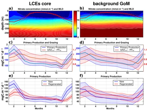
Figure 9: Climatological seasonal cycles of (a and b) nitrate concentration profiles (the red line overlaid is the average mixed layer depth), (c and d) the total primary production (blue) and the ratio of grazing rate over primary production (red) and (e and f) the new (blue) and regenerated (red) primary production. The left panels (a, c and e) refer to the seasonal time series in the LCEs core (r < 50 km) whereas the right panels (b, d and f) refer to the seasonal time series in the background GoM (r > 200 km). For each average cycle, the mean value is shown (full line) along with its variability (+/- 1 standard deviation relative to the mean, dashed lines).

The LCEs impact the upper ocean stratification (Fig 5.d), the nutricline depth (Fig 5.e) and consequently the nutrient supply to the euphotic layer (McGillicuddy et al., 2015). The relationship

Primary Production Primary Production

New Regenerated

New Regenerated

60 40 80 100 120 140 160

60 40 80 100 120 140 160

mgC.m².d¹⁻⁻

2 0

5 10 0 15

-50 -100 -150 -200 -250

depth (m)

Nitrate concentration (mmol.m ³) and MLD⁻ Nitrate concentration (mmol.m ³) and MLD⁻

mgC.m².d¹⁻⁻

Primary Production and Grazing

100 200

LCEs core background GoM

Months Months

Primary Production and Grazing 250

150 100

200 250

150

0.8 1 0.9 1.1

0.8 1 0.9 Primary Production 1.1 GRZtot : PPtot

Primary Production GRZtot : PPtot

a)

e) c)

f) d) b)

8 6 4 2

10 12 2 4 6 8 10 12

2 4 6 8 10 12 2 4 6 8 10 12

2 4 6 8 10 12 2 4 6 8 10 12

372 373

374

375 376 377 378 379 380

381 382

between mixed layer deepening and nutrient supply is studied here by comparing the ZNO3 with the MLD (Fig 9.a,b).

In late-spring and summer (from May to September), the water column is stratified (shallow MLD) and the downward displacement of the isopycnals within the LCEs pushes nutrients below the euphotic zone (see also Figs 5.e, 6.a): less nutrients are available within the LCE cores for

phytoplankton growth, explaining a deeper and less intense DCM. In winter, the convective mixing, fostered both by intense buoyancy losses and strong mechanical energy input at the surface, causes a larger deepening of the mixed layer within the LCEs core (~ - 125 m, Fig 9.a) compared to the background (~ - 85 m, Fig 9.b). This asymmetry is due to a pronounced decrease of the surface and subsurface stratification within the LCE core (Fig 5.d, Kouketsu et al., 2012). A quantitative diagnostic

of the stratification is given by the columnar buoyancy,

∫

0 H

N²(z).z.dz which measures the buoyancy

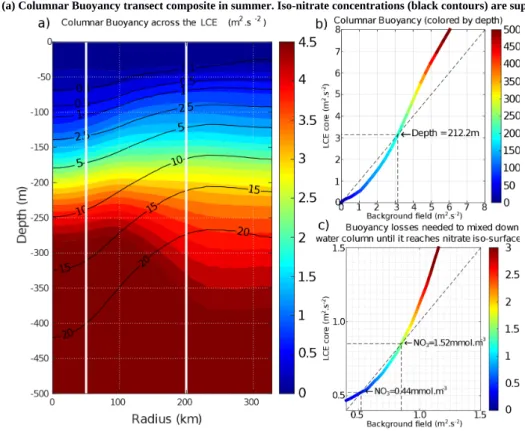
loss required to mix the water column to a depth H (Herrmann et al. 2008). Fig 10.a reveals significant differences in pre-winter buoyancy between the eddy core and its surroundings. Assuming that the change in buoyancy content is mainly controlled by the buoyancy flux at the surface (see Turner 1973;

Lascaratos & Nittis, 1998), it suggests that mixing the water column down to ~ -210 m depth requires smaller surface buoyancy loss in LCEs cores compared to the background GoM (Fig 10.b).

However, the larger winter deepening of the mixed layer within the LCEs core is not a sufficient condition to explain a larger nutrient supply. Indeed, it fosters the transport of nutrients from the nitracline toward the mixed layer because both are getting closer. Fig 10.c highlights that a smaller buoyancy loss mixes down the water column to greater nutrient concentration levels in the LCEs core 383

384

385 386 387 388 389 390 391 392

393

394 395 396 397 398

399 400 401 402

concentration within the LCEs (Fig 9.a). In addition, a diagnostic of the different contributions to [NO3] evolution is proposed in appendix B. It shows the dominant role of vertical advection and diffusion in winter in providing nutrients to the euphotic layer in the LCEs core.

Figure 10: (a) Columnar Buoyancy transect composite in summer. Iso-nitrate concentrations (black contours) are superimposed.

Vertical white lines delimit the three dynamical fields of the LCE composite. (b) Vertical increase of the columnar buoyancy in the LCEs core versus the background GoM. Colors refer to depth. (c) Columnar buoyancy loss required to mix the water column down to the iso-nitrate surface defined by the line color.

So far we have assumed that the surface buoyancy fluxes are identical over the LCEs core and the background GoM. However, this is not strictly the case because temperature/salinity features in the LCEs and background waters are different (Fig 5.b,c; see also Williams 1988). The modeled surface buoyancy loss during winter season is ~18 % more intense within the LCEs. This difference is substantial and probably mainly driven by additional surface cooling applied on the warm LCE core 404

405 406

407

408 409 410

411 412 413 414 415

through air-sea interaction. It contributes to enhance convection within the eddies core, and then nutrient supply toward the surface.

IV.3 Productivity

The primary productivity PPtot presents a clear seasonal cycle both in the LCEs cores and in the background GoM with lower values in October-November, a sharp increase starting in November, a maximum in February and a gradual decrease from March to October (Fig 9.c and 9.d). The pressure exerted by zooplankton grazers varies seasonally. It shows a similar seasonal cycle in the LCEs core and in the background GoM. On average, ~ 90% of the total daily growth is consumed by grazing, reaching the highest impact in March, just one month after the peak season of the PPtot in both LCEs dynamical areas. The annual PPtot is slightly lower in the LCEs core (~ 142.4 mgC·m^-2.d^-1) than in the background GoM (~ 148.9 mgC·m^-2.d^-1). The amplitude of the seasonal cycle is larger in the LCEs core: from April to November, PPtot is on average ~12% lower in the LCEs core whereas, in winter, PPtot is ~14% higher where it reaches ~ 243.2 mgC·m^-2.d^-1 in February.

The ratio of the PPNtot and PPRtot provides information about the mechanisms controlling the biomass growth (Fig 9.e and 9.f). In winter, the PPNtot plays a leading role, reaching up to 113-147 mgC·m^-2·d^-1, driven by the winter mixing and induced NO3 fluxes (see Appendix B). Conversely, the PPRtot is dominant from April to October. During this period, low NO3 resources are available in the euphotic layer and the ecosystem preferentially uses ammonium to sustain the PPtot. This seasonal pattern is characteristic of oligotrophic environments such as the GoM open waters (Wawrik et al., 2004; Linacre et al., 2015).

416 417

418

419 420 421 422 423 424 425 426 427 428

429 430 431 432 433 434 435

In winter, changes in PPtot are correlated to the intensity of winter mixing in the LCEs core (Fig 9.c) and the background GoM (Fig 9.d). The larger PPNtot in the eddy core is consistent with a larger supply of NO3 and evidences that the core of anticyclones can be preferential spots of enhanced biological production.

IV.4 How to explain summer productivity?

In summer, the total primary production is higher in the background GoM waters as the regenerated production rate is higher. But surprisingly, the new primary production exhibits similar rates in both regions, although NO3 depletion occurs deeper in the LCEs core. In the absence of a strong enough vertical mixing when the mixed layer is shallow, this apparent mismatch requires an additional mechanism, vertical advection, capable to supply NO3 to the euphotic layer (Sweeney et al., 2003; McGillicuddy et al., 2015).

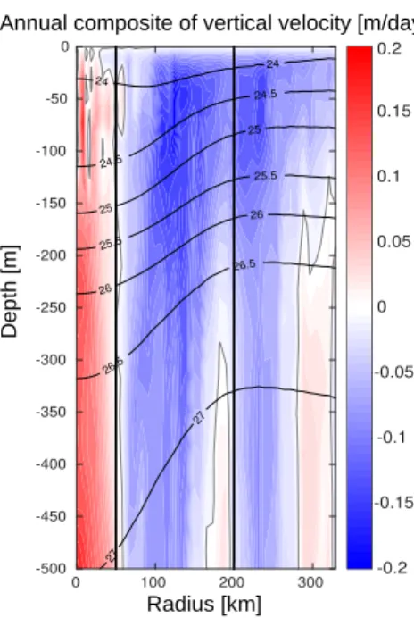
The model vertical velocity in the LCEs reveals an upward pumping in their core (Fig 11). The vertical velocity between 100 and 500 m is on average + 0.07 m·day^-1. This vertical transport is mainly driven by two mechanisms, eddy pumping (Falkowski et al., 1991) and eddy-wind interaction (Dewar and Flierl, 1987), but their relative importance is difficult to quantify (Gaube et al. 2014; McGillicuddy et al., 2015).

The eddy pumping mechanism is related to the decay of the rotational velocities from the moment LCEs are released from the Loop Current. In the LCE core, this decay is considered as moderate since lateral diffusivity is expected to be relatively low (section V.1). This process may however be considerable in the LCE ring where the erosion rates are important (Meunier at al., 2020).

436 437 438 439

440

441 442 443 444 445 446

447 448 449 450 451

452 453 454 455

Figure 11: Annually-averaged LCE composite transects of vertical velocities (m/day). Isopycnals anomalies (black contours) are superimposed on all panels. Vertical white lines delimit the three dynamical fields of the LCE composite.

Eddy-wind interactions are due to mesoscale modulation of the Ekman transport. Following the observation of a LCE core in quasi-solid body rotation, the horizontal vorticity varies little with the radius resulting in a negligible “non-linear” contribution of the Ekman pumping (McGillicuddy et al., 2008; Gaube et al., 2015). Assuming a small effect of the eddy SST-induced Ekman pumping, the total

Ekman pumping simplifies into its “linear” contribution computed as W_E= ∇× τ

ρ₀.(f+ζ ), where ρ0 is the surface density, f the Coriolis parameter, τ the stress at the sea surface depending on both the wind and ocean currents at the surface (Martin and Richards, 2001, equation 12) and ∇× the curl operator.

Considering uniform wind velocities ranging from 4.5 to 7.5 m·s^-1 (Nowlin & Parker, 1974;

Annual composite of vertical velocity [m/day]

Radius [km]

Depth [m]

456 457

458 459 460 461

462

463 464 465

surface circulation generated by the eddy. Its manifestation is a persistent horizontal divergence at surface balanced by an upward pumping in the eddy interior (see Martin & Richards, 2001; Gaube et al., 2013, 2014 for further details). With ρ0 ~ 1023 kg·m^-3 and f ~ 6.2.10^-5 s^-1, we estimate WE to be in the order of + 0.06-0.13 m·day^-1, in agreement with the modeled vertical velocity within the core. The Ekman-eddy pumping mechanism could explain a large fraction of the gradual upwelling of isopycnals within the eddy’s core and may actively contribute to the advective vertical flux of nutrients (see Appendix B). In summer, this mechanism could explain why new primary production rates are similar in the LCEs core and the background GoM waters although the nutrient pool is located much deeper in the LCEs core.

The eddy-Ekman pumping persists in the LCEs core throughout their lifetime as long as there is a wind stress applied at the surface. During wintertime, we expect that both vertical mixing and eddy- Ekman pumping participate to increase the new primary production. A question then arises on the relative contribution of winter mixing to eddy-Ekman pumping in the LCEs core primary production increase in winter. This issue was tackled by He et al. (2017) and Travis et al. (2019) comparing the rate of change of the mixed layer depth with the vertical velocity induced by the eddy-Ekman pumping (equation 4 in He et al, 2017). In the LCEs core, we estimate the mixed layer to deepen at roughly 0.8 m·day^-1, which is on average about 10 times larger than pumping mechanism. This supports winter mixing as the overwhelming process for the LCEs-induced primary production peak in winter.

V/ Summary and perspectives

The [CHL] variability induced by the mesoscale Loop Current Eddies in the Gulf of Mexico is studied by analyzing vortex composite fields generated from a coupled physical-biogeochemical model 467

468 469 470 471 472 473 474 475

476 477 478 479 480 481 482 483 484

485

486 487

at 1/12° horizontal resolution. LCEs are hotspots for mesoscale biogeochemical variability. Despite the [CHL]surf negative anomaly associated with their core (r < 50 km), model results indicate that LCEs are associated with enhanced phytoplankton biomass content, particularly in winter. This enhancement results from the contribution of multiple mechanisms of physical-biogeochemical interactions and contrasts with the background oligotrophic surface waters of the GoM.

The main results of this study are:

 LCEs cores present a negative surface chlorophyll anomaly,

 Unlike [CHL]surf, [CHL]tot is larger in the LCEs cores compared to the background GoM in winter.

 LCEs core trigger a large phytoplankton biomass increase in winter,

 The winter mixing is a key mesoscale mechanism that preferentially supplies nutrients to the euphotic layer within the LCEs core. Consequently, it drives an eddy-induced peak of new primary production,

 Ekman-eddy pumping is a significant mechanism for sustaining relatively high new primary production rates within LCE cores during summer.

The phytoplankton biomass increase in individual LCEs cores suggests that LCEs play an important role in sustaining the large-scale GoM productivity.

Although the biological response to LCEs may present some specificities due to the particular dynamical nature of LCEs, this study suggests potentially generic insights on the biogeochemical role that anticyclonic eddies could play in oligotrophic environments. It echoes the previous works of Martin and Richards (2001), Gaube et al. (2014, 2015) and especially Dufois et al. (2014, 2016) and He et al. (2017) who proposed winter vertical mixing as an explanation for the positive [CHL]surf anomaly 488

489 490 491 492

493 494 495 496 497 498 499 500 501 502 503 504

505 506 507 508 509

from our results is that the enhanced primary production and biomass content within anticyclonic eddies may not necessarily be correlated with the surface layer variability. In oligotrophic areas, the integrated content of chlorophyll in the water column has to be considered. This implies that caution should be exercised in the analysis and interpretation of [CHL]surf observed by remote sensing instruments and highlights the crucial need for in-situ biogeochemical and bio-optical measurements.

In oligotrophic environments, defined by their low production rates and their low chlorophyll concentration, anticyclonic eddies are able to trigger local enhanced biological productivity and generate phytoplankton biomass positive anomalies. In a scenario of expansion of oligotrophic areas (Barnett et al., 2001; Behrenfeld et al., 2006; Polovina et al., 2008), the fate and role of mesoscale anticyclones is an important aspect to be considered.

This study focuses on mesoscale physical-biogeochemical interactions which is the spectral range resolved by GOLFO12-PISCES configuration. To go further into the analysis of anticyclonic eddies in oligotrophic environments, the role of submesoscale is of particular interest since it has been proved to trigger mechanisms of significance importance for biogeochemistry (Levy et al., 2018).

Higher model resolutions can locally enhanced density gradients (Levy et al., 2012; Omand et al., 2015) leading to ageostrophic circulations that perturbs the circular flow around vortices (Martin and Richards, 2001) or enhanced vertical velocities that potentially foster the nutrient supply to the euphotic layer. Beside the mesoscale Ekman pumping located at the eddy center, eddy-wind

interactions also produce vertical velocities at the eddy periphery (e.g. Flierl and McGillicuddy, 2002).

Finally, it is also worth noting that anticyclonic mesoscales eddies are capable of trapping near-inertial energy waves in the ocean (Kunze 1985, Danioux et al. 2008, Koszalka et al. 2010, Pallas-Sanz et al., 2016) where they produce vertical recirculation patterns (Zhong and Bracco, 2013). Even if, some of these dynamical aspects are partially resolved at 1/12° horizontal resolution, higher resolutions simulations are necessary to correctly assess their specific impact.

511 512 513 514 515 516 517 518 519 520

521 522 523 524 525 526 527 528 529 530 531 532 533 534

Acknowledgments: Research funded by the National Council of Science and Technology of Mexico –

Mexican Ministry of Energy – Hydrocarbon Trust, project 201441. This is a contribution of the Gulf of Mexico Research Consortium (CIGoM). We acknowledge the provision of supercomputing facilities by CICESE.

535 536 537 538

APPENDIX A: CHL/C-biomass ratio and ecosystem structure

[CHL] is widely used as a proxy for phytosynthetic biomass (Strickland, 1965; Cullen, 1982).

However, in addition to depend on phytoplankton concentration, it is also affected by several other factors mainly produced by intracellular physiological mechanisms (Geider, 1987). In particular, photoacclimation processes have been proved to be determinant to explain [CHL]surf variability in oligotrophic areas (Mignot et al. 2014). In the GoM open-waters, this issue was specifically addressed at a basin scale in Pasqueron de Fommervault et al. (2017) considering in-situ particulate

backscattering measurements and in Damien et al. (2018) from modeling tools. They both reach the same conclusion: [CHL]tot variability provides a reasonably good estimate of the total C-biomass variability ([PHY]tot).

This is confirmed by the small amplitude of the seasonal cycle of the ratio [CHL]tot/[PHY]tot in the background GoM (0.256 +/- 0.004 g·mol^-1 averaged throughout the year, Fig A1). In the LCEs core, this statement is still valid but must be qualified, since the ratio [CHL]tot/[PHY]tot presents small but significant changes through the year (Fig A1.a). It is around 0.24 g·mol^-1 from March to November and increases sharply in December to reach about 0.32 g·mol^-1 in January and February. As a result, in winter, the photoacclimation mechanism accounts for ~25% of the total [CHL]tot increase (the

remaining part being an effective phytoplankton biomass increase). In summer, the ratio [CHL]tot/[PHY]tot is slightly lower in the LCEs core compared to the background GoM. As a

consequence, the [CHL]tot negative anomaly associated with LCEs core does not necessarily translate into a [PHY]tot negative anomaly.

Overall in the GoM open-waters, there is a dominance of the small-size phytoplankton over the large-size class in proportion closed to 80%-20% (Linacre et al., 2015). Although the modeled 539

540 541 542 543 544 545 546 547 548

549 550 551 552 553 554 555 556 557 558

559 560

ecosystem structure is relatively simple, this typical community size structure is well reproduced by GOLFO12-PISCES (Fig A1.c and A1.d), that also suggests a shift in the ecosystem structure in winter.

The different response among size classes results from the enhancement of nutrient vertical flux. The role of “secondary” nutrient in this change in the community composition must not be overlooked also, in particular for diatoms (accounted in the model’s large-size group) since they also uptake on silicate (Benitez-Nelson et al., 2007). Moreover, GOLFO12-PISCES exhibits a modulation of the ecosystem structure by LCEs. The dominance of small-size phytoplankton is slightly more marked in summer and the winter shift is stronger in the LCEs core.

Figure A1: Climatological seasonal cycles of (a and b) the CHL/C-biomass ratio and (c and d) the vertically integrated content of phytoplankton concentration (small size in blue, large size in red). The left panels (a and c) refer to the time series in the LCEs core (r < 50 km) whereas the right panels (b and d) refer to the time series in the background GoM (r > 200 km). For each average cycle, the average value is shown (full line) along with its variability (+/- 1 standard deviation relative to the mean, dashed lines).

Months Months

LCEs core background GoM

Small Large

80 100 120

80 100 120

0 20 40

0 20 40 Phytoplankton concentration (mmol.m ²)⁻ Phytoplankton concentration (mmol.m ²)⁻

CHL/C-biomass ratio (g.mol ¹)⁻ CHL/C-biomass ratio (g.mol ¹)⁻

0.2 0.3

0.2 0.3

Small Large

a) b)

c) d)

2 4 6 8 10 12 2 4 6 8 10 12

2 4 6 8 10 12 2 4 6 8 10 12

561 562 563 564 565 566 567 568

569 570 571 572 573

APPENDIX B : Nitrate budget at a seasonal scale

Nutrients availability in the euphotic layer is a key mechanism to trigger biomass increase in LCEs. The processes driving the seasonality of nutrient concentrations are here investigated diagnosing the different contributions to nitrate concentrations (hereafter [NO3]) variability. The goal is to confirm the vertical transport of nutrients and quantify the budget in order to determine the driving mechanisms.

The analysis is restricted to nitrate concentrations, considered as the main limiting factor for large size- class phytoplankton growth in the GoM (Myers et al., 1981; Turner et al., 2006), although phosphates and silicates are also modeled. We do not exclude that phosphates or silicates could also play a significant role. In cylindrical coordinates, the [NO3] equation reads:

∂ NO3

∂ t =−V_r∂ NO3

⏟

radial advection

− Vθ

r

∂ NO3

⏟

azimuthal advection

−V_z∂ NO3

⏟

vertical advection

+Dl

r

∂

∂ r

(

)

⏟

lateral diffusion

+ ∂

∂ z

(

)

⏟

vertical diffusion

+ SMS

⏟

Sourcemenus sink

+Asselin

.

Basically, this is a 3D advection-diffusion equation with added "sources and sinks" terms, namely biogeochemical release and uptake rates. One must include also an "Asselin term", a modeling artifact due to the Asselin time filtering. We focus on the seasonal cycle of three particular trend terms: the vertical mixing (Fig B1.a and B1.b), the vertical advection (Fig B1.c and B1.d) and a "source menus sink" term (Fig B1.e B1.f).

[NO3] variations from vertical dynamics are mainly positive, especially in the first 100 m of the water column. This traduces in year-round NO3 source driven by physical processes. By contrast, biogeochemical processes consume NO3 in the upper layer to sustain the primary production (Fig B1.e and B1.f). In the sub-surface layer (~ below the isoline on which nitrate concentration is equal to 2 mmol.m^-3), the process of nitrification constitutes a biological source of [NO3]. To first order, this 574

575 576 577 578 579 580 581 582

583

584 585 586 587 588

589 590 591 592 593

represents the global functioning of the ecosystem, valid in both fields and throughout the year.

However, the seasonal cycle strongly influence the magnitude of these trend terms, in particular in the LCE core.

In winter, from December to February, vertical advective and diffusive motions produce an increase of [NO3] within the mixed layer. This tendency consists in an advective entrainment resulting from the deepening of the mixed layer which mainly acts to increase [NO3] at the base of the mixed layer (Fig B1.c and B1.d) and vertical mixing which redistributes vertically the nutrients and tends to homogenize [NO3] in the mixed layer (Fig B1.a and B1.b). The winter [NO3] increase is most important in the LCE core at the base of the mixed layer (~ + 6.5.10^-7 mmol·m^-3·d^-1, nearly 3 times larger than in the background GoM), attesting here a preferential NO3 uplift due to deeper convection. Integrated over the mixed layer, the winter vertical fluxes produce [NO3] enhancement of ~ 2.4.10^-5 mmol·m^-2·d^-1 in the eddy core whereas it is only of ~ 1.6.10^-5 mmol·m^-2·d^-1 in the background GoM. This also explains why, on average, the density/nitrate relation differs in the LCEs core (Fig 5.e). In response, the [NO3] tendency due to biogeochemical processes indicates an increase of the [NO3] uptake. This increase is about 1.5 times larger in the core (~ - 1.3.10^-3 mmol·m^-2·d^-1 integrated over the mixed layer) than in the background GoM (~ - 0.9.10^-3 mmol·m^-2·d^-1). Knowing that it feeds biomass production, this [NO3] loss is consistent with the primary production peak in winter (Fig 9.e and 9.f).

In summer, [NO3] variations due to vertical processes are smaller than in winter. They are also weaker in the LCEs core upper layer (almost nil in the 0-50m layer) compared to the background GoM, consistent with a deeper NO3 pool and a shallow mixer layer. In the eddy core, one can assume that the NO3 vertical supply is entirely consumed before reaching 50m. Below 50m, vertical [NO3] diffusive trends are consistently more important in the background GoM, in agreement with a steeper nitracline 594

595 596

597 598 599 600 601 602 603 604 605 606 607 608 609 610 611 612 613 614 615 616