Sea‑ice properties and nutrient concentration as drivers of the taxonomic and trophic structure of high‑Arctic protist and metazoan communities

(1)

https://doi.org/10.1007/s00300-019-02526-z ORIGINAL PAPER

Sea‑ice properties and nutrient concentration as drivers of the taxonomic and trophic structure of high‑Arctic protist and metazoan communities

Hauke Flores^1,2 · Carmen David^1,2,3 · Julia Ehrlich^1,2 · Kristin Hardge¹ · Doreen Kohlbach^1,2 · Benjamin A. Lange^1,2,4 · Barbara Niehoff¹ · Eva‑Maria Nöthig¹ · Ilka Peeken¹ · Katja Metfies^1,5

Received: 10 January 2019 / Revised: 14 June 2019 / Accepted: 18 June 2019 / Published online: 28 June 2019

Abstract

In the Arctic Ocean, sea-ice decline will significantly change the structure of biological communities. At the same time, changing nutrient dynamics can have similarly strong and potentially interacting effects. To investigate the response of the taxonomic and trophic structure of planktonic and ice-associated communities to varying sea-ice properties and nutrient concentrations, we analysed four different communities sampled in the Eurasian Basin in summer 2012: (1) protists and (2) metazoans from the under-ice habitat, and (3) protists and (4) metazoans from the epipelagic habitat. The taxonomic composition of protist communities was characterised with 18S meta-barcoding. The taxonomic composition of metazoan communities was determined based on morphology. The analysis of environmental parameters identified (i) a ‘shelf-influenced’

regime with melting sea ice, high-silicate concentrations and low NOx (nitrate + nitrite) concentrations; (ii) a ‘Polar’ regime with low silicate concentrations and low NO_x concentrations; and (iii) an ‘Atlantic’ regime with low silicate concentrations and high NO_x concentrations. Multivariate analyses of combined bio-environmental datasets showed that taxonomic community structure primarily responded to the variability of sea-ice properties and hydrography across all four communities.

Trophic community structure, however, responded significantly to NOx concentrations. In three of the four communities, the most heterotrophic trophic group significantly dominated in the NO_x-poor shelf-influenced and Polar regimes compared to the NO_x-rich Atlantic regime. The more heterotrophic, NO_x-poor regimes were associated with lower productivity and carbon export than the NOx-rich Atlantic regime. For modelling future Arctic ecosystems, it is important to consider that taxonomic diversity can respond to different drivers than trophic diversity.

Keywords Arctic Ocean · Sea ice · Community structure · Protists · Zooplankton · Under-ice fauna · Nutrients · Trophic ecology

Introduction

The Arctic Ocean has been experiencing a rapid decline in sea-ice volume (Kwok and Rothrock 2009; Laxon et al.

2013) and sea-ice extent over the past two decades (Serreze et al. 2007; Stroeve et al. 2012; Simmonds 2015). Model

Electronic supplementary material The online version of this article (https ://doi.org/10.1007/s0030 0-019-02526 -z) contains supplementary material, which is available to authorized users.

* Hauke Flores hauke.flores@awi.de

1 Section Polar Biological Oceanography, Alfred Wegener Institut Helmholtz-Zentrum für Polar- und Meeresforschung, Bremerhaven, Germany

2 Centre for Natural History (CeNak), University of Hamburg, Zoological Museum, Hamburg, Germany

3 Institut Français de Recherche Pour l’Exploitation de la Mer (Ifremer), Plouzané, France

4 Fisheries and Oceans Canada, Freshwater Institute, Winnipeg, MB, Canada

5 Helmholtz Institute for Functional Marine Biodiversity (HIFMB), Oldenburg, Germany

(2)

simulations have indicated that an ice-free Arctic Ocean during summer is likely to occur by the mid of the twenty- first century (Wang and Overland 2009; Stroeve et al. 2012).

In the water column, significant environmental changes are expected to occur, such as an increase in surface water temperatures, changing circulation patterns, increased ocean acidification, enhanced stratification, and nutrient limitation (IPCC 2014). These changes will profoundly impact on ecosystem structure and function, such as carbon and nutrient cycling, carbon export, and availability of marine- living resources. Studies on Arctic plankton communities have demonstrated ongoing change in community composition and in the distribution of ecological key species related to ocean warming and sea ice decline (e.g. Bluhm et al. 2011; Wassmann 2011; Wassmann et al. 2011; Kraft et al. 2013; Nöthig et al. 2015; Hardge et al. 2017a, b). Sea- ice decline has been linked to enhanced pelagic primary production (Arrigo and van Dijken 2011, 2015), mainly due to increased light availability (Nicolaus et al. 2012). In contrast, increased freshwater input due to river runoff may result in decreased primary production, because of lower nutrient availability (Yun et al. 2016). Besides nutrient supply, other factors are also likely to affect Arctic ecosystem structure, such as oceanic CO₂ uptake and increased temperatures (Tremblay et al. 2015).

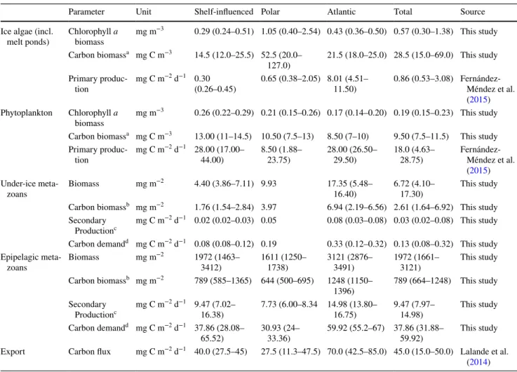
In the central Arctic Ocean, the bulk of the total primary production is often generated by sea-ice algae rather than phytoplankton (Gosselin et al. 1997; Fernández-Méndez

et al. 2015). Reduced sea-ice algae production due to habitat/substrate loss can influence fundamental patterns of carbon flux in the food web. Recently, it was shown that abundant ecological key species, such as Calanus spp. and juvenile polar cod Boreogadus saida, significantly depend on carbon produced by ice algae (Budge et al. 2008; Søreide et al. 2010; Wang et al. 2015; Kohlbach et al. 2016, 2017).

Kohlbach et al. (2016) demonstrated that the cumulative carbon demand by metazoan grazers far exceeded primary production rates by phytoplankton and sea-ice algae during summer. This suggests that intermediate trophic levels of the food web depend on heterotrophic carbon sources to a much greater extent than previously suggested (David et al.

2015; Kohlbach et al. 2016). While the transformation of Arctic sea-ice habitats continues, increased dependency on heterotrophic carbon transmitters may be a significant factor changing the trophic functioning of biological communities in the future Arctic Ocean.

In summer 2012, the lowest sea-ice extent since the beginning of satellite-based observations was recorded in the Arctic Ocean (Parkinson and Comiso 2013). In the Eurasian Basin of the Arctic Ocean, a vast area of rapidly degrading sea ice opened up in regions that are normally ice- covered year-round (Fig. 1; Stroeve et al. 2012; Boetius et al.

2013). Interacting with the anomalous 2012 sea ice situation was a contrast between nutrient-rich Atlantic Water entering through the Fram Strait, nutrient-depleted Polar Water advected from the central Arctic Ocean, and shelf-influenced

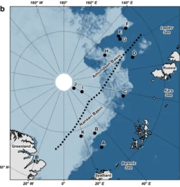
Fig. 1 Overview of the research area with sampling locations and major topographic features. Sea-ice concentration derived from SSMIS satellite data (www.meere ispor tal.de) is shown on 14th of

August (a) and 13th of September 2012 (b). Capital letters indicate sampling locations from Table 1

(3)

water from the Laptev Sea (Lalande et al. 2014; David et al.

2015; Fernández-Méndez et al. 2015; Metfies et al. 2016).

Sampling this unprecedented situation of extreme reduction of sea ice during Polarstern expedition PS80 gave the unique opportunity to sample both protist and metazoan communities simultaneously with hydrographical conditions, nutrient concentrations and sea-ice properties.

Changes in the taxonomic and trophic structure of these communities can have a strong impact on key ecosystem functions, such as primary and secondary production, carbon-, and nutrient cycling. The rapid environmental changes in the Arctic Ocean likely act differently on sea ice-associated communities compared to planktonic communities. In high-Arctic ecosystems, however, the response of biological communities to different drivers interacting with each other is poorly understood, especially in the under-ice habitat (Wassmann et al. 2011). In this study, we use a range of morphological, molecular, and statistical tools to analyse the structure of protist and metazoan communities both in the under-ice habitat and in the epipelagic habitat in the Eura- sian Basin of the Arctic Ocean. We hypothesize that (1) the structure of both protist and metazoan communities responds to similar environmental drivers in each habitat; and (2) that changes in taxonomic composition in relation to environmental variability will be resembled in the trophic structure of these communities. To test these hypotheses, we:

(a) identified physical–chemical drivers structuring environmental regimes, such as sea-ice properties, hydrography and nutrient concentrations;

(b) analysed the relationship of the taxonomic composition of Arctic protist and metazoan communities with these environmental drivers;

(c) investigated if environmental drivers were associated with both the taxonomic and the trophic community structure.

Material and methods

Research area

The samples were collected from 7 August to 29 Septem- ber 2012 during the RV Polarstern expedition PS80 (ARK- XXVII/3, “IceArc”) in the central Arctic Ocean (Fig. 1).

The area sampled extended over the Eurasian Basin, ranging from 82° to 89°N, and from 30° to 130°E, and was entirely situated in deep-sea waters (depth range 3409–4384 m;

Table 1). Samples and data were collected with various sampling gear at altogether 46 stations. For the purpose of this study, we grouped these stations into 11 locations identified by the letters A to K, based on spatio-temporal proximity. Most sampling locations were associated with

drifting sea-ice stations. The sampling around these locations, therefore, extended over a period of up to 3 days, and covered a latitudinal drift distance of up to 14.5 nm (28 km).

A complete account of all stations sampled for this study was provided in Table 1.

Sampling of environmental parameters Water column

A conductivity temperature depth probe (CTD) with a carou- sel water sampler was used to collect environmental parameters from the water column. The CTD (Seabird SBE9+) was equipped with a fluorometer (Wetlabs FLRTD), a dissolved oxygen sensor (SBE 43) and a transmissiometer (Wetlabs C-Star). Details of the CTD sampling procedure were provided by Boetius et al. (2013). Data are available online in the PANGAEA database (Rabe et al. 2012). Nutrient samples were collected at multiple depths, and analysed in an air-conditioned lab container with a continuous flow auto analyser (Technicon TRAACS 800) following the procedure described by Boetius et al. (2013). Measurements were made simultaneously on four channels: PO₄, Si, NO₂ + NO₃ together and NO₂ separately. Nutrient values for the purpose of this study were taken from the depth of the chlorophyll a maximum. The depth of the upper mixed layer (MLD) was calculated from the ship CTD profiles after Shaw et al.

(2009). Integrated values for water temperature and salinity within the MLD were derived by averaging continuous CTD profile data between the surface and the MLD. A stratification index was estimated as the density gradient between the density of the mixed layer and the density of the water 5 m below the MLD.

Under‑ice habitat

Under-ice metazoans and environmental parameters of the ice–water interface layer (0–2 m) were sampled with a Sur- face and Under-Ice Trawl (SUIT) (van Franeker et al. 2009).

The SUIT consisted of a steel frame with a 2 m × 2 m opening and two parallel 15 m-long nets attached: (1) a 7 mm half-mesh commercial shrimp net, which covered 1.5 m of the opening width; and (2) a 0.3 mm mesh zooplankton net, which covered 0.5 m of the opening width. SUIT haul dura- tions varied between 17 and 42 min (mean = 29 min) over an average distance of 1.5 km. Water inflow speed and direction were calculated using a Nortek Aquadopp® Acoustic Dop- pler Current Profiler (ADCP). The trawled area was calculated by multiplying the distance trawled in water, estimated from ADCP data, with the net width. The SUIT sampling technique and performance has been described in detail by David et al. (2015) and Flores et al. (2012). A sensor array was mounted on the SUIT frame, comprising among

(4)

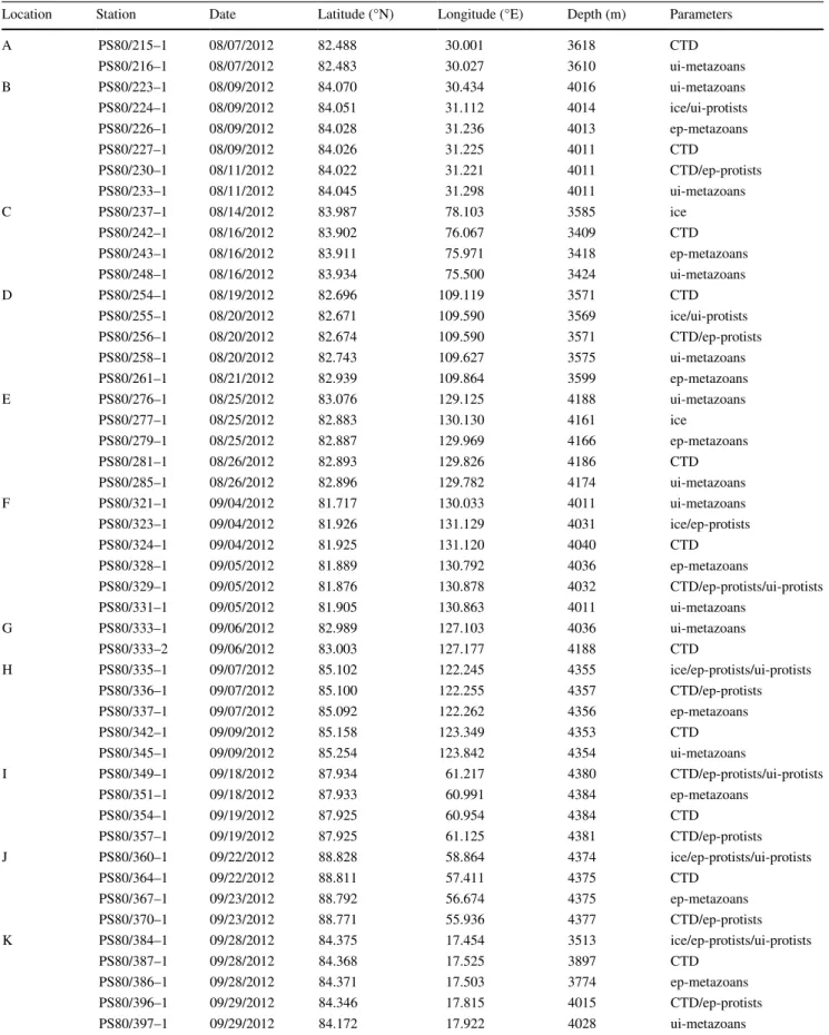
Table 1 Stations sampled during the expedition PS80. Nearby stations were grouped together as ‘locations’ represented by letters A to K

CTD water column parameters sampled with the ship’s CTD (temperature, salinity, nutrients), ice sea-ice parameters, ui under ice, ep epipelagic

Location Station Date Latitude (°N) Longitude (°E) Depth (m) Parameters

A PS80/215–1 08/07/2012 82.488 30.001 3618 CTD

PS80/216–1 08/07/2012 82.483 30.027 3610 ui-metazoans

B PS80/223–1 08/09/2012 84.070 30.434 4016 ui-metazoans

PS80/224–1 08/09/2012 84.051 31.112 4014 ice/ui-protists

PS80/226–1 08/09/2012 84.028 31.236 4013 ep-metazoans

PS80/227–1 08/09/2012 84.026 31.225 4011 CTD

PS80/230–1 08/11/2012 84.022 31.221 4011 CTD/ep-protists

PS80/233–1 08/11/2012 84.045 31.298 4011 ui-metazoans

C PS80/237–1 08/14/2012 83.987 78.103 3585 ice

PS80/242–1 08/16/2012 83.902 76.067 3409 CTD

PS80/243–1 08/16/2012 83.911 75.971 3418 ep-metazoans

PS80/248–1 08/16/2012 83.934 75.500 3424 ui-metazoans

D PS80/254–1 08/19/2012 82.696 109.119 3571 CTD

PS80/255–1 08/20/2012 82.671 109.590 3569 ice/ui-protists

PS80/258–1 08/20/2012 82.743 109.627 3575 ui-metazoans

PS80/261–1 08/21/2012 82.939 109.864 3599 ep-metazoans

E PS80/276–1 08/25/2012 83.076 129.125 4188 ui-metazoans

PS80/277–1 08/25/2012 82.883 130.130 4161 ice

PS80/279–1 08/25/2012 82.887 129.969 4166 ep-metazoans

PS80/281–1 08/26/2012 82.893 129.826 4186 CTD

PS80/285–1 08/26/2012 82.896 129.782 4174 ui-metazoans

F PS80/321–1 09/04/2012 81.717 130.033 4011 ui-metazoans

PS80/323–1 09/04/2012 81.926 131.129 4031 ice/ep-protists

PS80/324–1 09/04/2012 81.925 131.120 4040 CTD

PS80/328–1 09/05/2012 81.889 130.792 4036 ep-metazoans

PS80/329–1 09/05/2012 81.876 130.878 4032 CTD/ep-protists/ui-protists

PS80/331–1 09/05/2012 81.905 130.863 4011 ui-metazoans

G PS80/333–1 09/06/2012 82.989 127.103 4036 ui-metazoans

PS80/333–2 09/06/2012 83.003 127.177 4188 CTD

H PS80/335–1 09/07/2012 85.102 122.245 4355 ice/ep-protists/ui-protists

PS80/337–1 09/07/2012 85.092 122.262 4356 ep-metazoans

PS80/342–1 09/09/2012 85.158 123.349 4353 CTD

PS80/345–1 09/09/2012 85.254 123.842 4354 ui-metazoans

I PS80/349–1 09/18/2012 87.934 61.217 4380 CTD/ep-protists/ui-protists

PS80/351–1 09/18/2012 87.933 60.991 4384 ep-metazoans

PS80/354–1 09/19/2012 87.925 60.954 4384 CTD

J PS80/360–1 09/22/2012 88.828 58.864 4374 ice/ep-protists/ui-protists

PS80/364–1 09/22/2012 88.811 57.411 4375 CTD

PS80/367–1 09/23/2012 88.792 56.674 4375 ep-metazoans

K PS80/384–1 09/28/2012 84.375 17.454 3513 ice/ep-protists/ui-protists

PS80/387–1 09/28/2012 84.368 17.525 3897 CTD

PS80/386–1 09/28/2012 84.371 17.503 3774 ep-metazoans

PS80/397–1 09/29/2012 84.172 17.922 4028 ui-metazoans

(5)

other devices a CTD probe with built-in fluorometer and an altimeter used to derive ice thickness profiles and under-ice chlorophyll a concentrations (David et al. 2015). Gridded daily sea-ice concentrations for the Arctic Ocean derived from SSMIS satellite data using the algorithm specified by Spreen et al. (2008), were downloaded from the sea-ice por- tal hosted at the University of Bremen (www.meere ispor tal.de). For each sea-ice station, sea-ice concentration was averaged from nine adjacent grid cells, with the grid cell in which the station was situated as the centre. A detailed description of environmental sampling and parameter esti- mations was provided by David et al. (2015). An overview of the environmental parameters and their ranges was provided in Table 2.

Chlorophyll a concentration

Particulate organic matter (POM) from water samples was collected on Whatman GF/F glass fibre glass fibre filters (0.7 µm), extracted in 90% acetone and analyzed with a Turner-Design fluorometer according to standard procedure (Edler 1979; Evans et al. 1987). Calibration of the fluorometer was carried out with standard solutions of Chlorophyll a (Sigma, Germany). To estimate chlorophyll a content of sea ice, ice cores were collected at each ice stations using a 9 cm-diameter ice corer (Kovacs). Ice cores were cut in seg- ments, which were each melted in 4 °C with 0.2 µm filtered sea water in the dark. For details of sea-ice sampling see Boetius et al. (2013) and Lange et al. (2016). For pigment analysis of filtered ice core samples to each filter 50 µl inter- nal standard (canthaxanthi), 1.5 ml acetone and small glass beads were added and the samples kept frozen at – 20 °C for 15 min. Cell were disrupted for 20 s with a Precellys® tis- sue homogenizer. The centrifugation of the extract was performed in a cooled centrifuge (0°) and the supernatant liquid was kept and filtered through a 17 mm HPLC 0.2 µm PTFE

filter (LABSOLUTE). Pigment measurement was carried out with a Waters HPLC-system equipped with an auto sampler (717 plus), a pump (600), a Photodiode array detector (2996), a fluorescence detector (2475) and the EMPOWER software. The analysis of the pigments was conducted by reverse-phase HPLC, with a VARIAN Microsorb-MV3 C8 column (4.6 × 100 mm) and HPLC-grade solvent (Merck).

For details see Kilias et al. (2013).

Sampling of organisms from the under‑ice and the pelagic habitats

Protists

Sampling of epipelagic protists was carried out with a rosette sampler equipped with 24 Niskin bottles attached to the ship CTD. Samples were taken during the up-cast at the vertical maximum of chlorophyll a fluorescence determined during the downcast. The sampling depth varied between 10 and 50 m. Two-litre subsamples were transferred into PVC bottles. Under-ice protist samples were collected with a Kemmerer bottle (6.3 l) lowered through an ice hole directly below the ice. Protists were collected for molecular analyses by sequential filtration of one water sample through three different mesh sizes (10 µm, 3 µm, 0.4 µm) at a vacuum pressure of − 200 mbar using Isopore Membrane Filters (Millipore, USA). Filters were stored in Eppendorf tubes (Eppendorf, Germany) at − 80 °C until further processing in the laboratory.

In this study, we used a subset of an 18S meta-barcoding- data set comprising a total of 56 samples collected in different ice-influenced habitats (Hardge et al. 2017a). DNA samples were processed as described in Hardge et al. (2017a).

DNA extraction was carried out with the NucleoSpin® Plant II kit (Macherey–Nagel) following the manufacturer’s protocol. The V4 region was amplified in triplicates using the

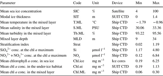
Table 2 Environmental parameters used in analyses

Chl a chlorophyll a, Min minimum value, Max maximum value

Parameter Code Unit Device Min Max

Mean sea ice concentration SIC % Satellite 4 100

Modal ice thickness SIT m SUIT CTD 0 1.4

Mean temperature in the mixed layer T.ML °C Ship CTD − 1.79 − 0.96

Mean salinity in the mixed layer S.ML PSU Ship CTD 30.06 33.36

Mean turbidity in the mixed layer Tb.ML % Ship CTD 93.22 95.56

Mixed layer depth MLD m Ship CTD 9 34

Stratification index Strat Ship CTD 0.02 1.19

SiO₄²⁻ conc. at the chl a maximum Si µmol l⁻¹ Ship CTD 1.17 4.80 NO₃²⁻ + NO₂³⁻ conc. at the chl a maximum NOx µmol l⁻¹ Ship CTD 0.12 6.84 Mean chlorophyll a conc. in sea ice Chl.ice mg m⁻³ Ice cores 0.19 6.25 Mean chl a conc. in the under-ice habitat Chl.ui mg m⁻³ SUIT CTD 0.19 1.13 Mean chl a conc. in the mixed layer Chl.ML mg m⁻³ Ship CTD 0.06 0.30

(6)

universal primer set TAReuk454FWD1 and TAReukREV3 (Stoeck et al. 2010). The DNA amplification was carried out in two rounds using a Mastercycler (Eppendorf, Germany).

Resulting PCR products were purified with NucleoSpin®

Gel & PCR Clean up kit (Macherey–Nagel) according to the manufacturer’s protocol. Pooled triplicates were sequenced on the MiSeq 18S meta-barcoding platform (2 × 300 paired-end reads). The library preparation was done with the TruSeq RNA Library Preparation Kit v2 according to the manufacturer’s protocol. We used QIIME version 1.8.0 (Caporaso et al. 2010) for sequence analysis. Operational taxonomic units (OTUs) were determined de novo at a minimum similarity threshold of 98%. According to Bokulich et al. (2013), OTUs consisting of less than 0.005% of processed sequences were removed. Representative sequences of each OTU were aligned with the bioinformatics pipeline called PhyloAssigner (Vergin et al. 2013). The compiled reference database is available on request in ARB-format.

164 of the 210 protist taxa identified with sequence analysis were assigned to the trophic groups “autotrophs”, “mixotrophs” and “heterotrophs” based on published knowledge on their trophic function (Online Resource ESM1). Based on the relative sequence abundance of combined OTUs with identical taxonomic labels, the proportional contribution of autotrophs, mixotrophs and heterotrophs was calculated for each sampling location.

Metazoans

Under-ice metazoans were sampled with the SUIT. After retrieval of the catch from the SUIT, the material was preserved in 4% formaldehyde/seawater solution for quantita- tive analysis. The samples were analysed for species composition and abundance at the Alfred Wegener Institute following the procedure described by David et al. (2015).

In all macrofauna species, total body length was measured to the nearest 1 mm using a stereo microscope coupled to a digital image analysis system (Leica Model M 205C and image analysis software LAR 4.2). Copepods were classified by developmental stage and sex. Epipelagic metazoans were sampled with a Multinet (Hydrobios, Kiel). The Multinet had a mouth opening area of 0.25 m² and was equipped with five nets (150 µm), which were sequentially opened and closed to five sample discrete depth intervals (1500–1000–500–200–50–0 m). In the present study, only samples from the uppermost depth stratum (0–50 m) were considered. The samples were preserved in 4% formaldehyde/seawater solution buffered with borax. In the laboratory, the samples were subdivided with a plankton splitter (Hydrobios) usually to 1/8 and at maximum to 1/64. Abun- dant species (n > 50 in an aliquot) were sorted only from one subsample, while less abundant species were sorted from at least two subsamples. Areal abundances (ind. m⁻²) were

calculated by dividing the total number of animals in each net by the water volume filtered, and multiplying the resulting volumetric density by the vertical depth range sampled.

We estimated the individual dry mass of freeze-dried SUIT samples of the five most abundant amphipod species. To account for the high variability in size distribution between sampling sites of the amphipod Themisto libellula, a size-dry weight relationships was established. This relationship was then used to estimate the dry mass of Themisto spp. at each station based on their total biovolume and mean size, respectively. Dry mass of Calanus copepods was estimated based on size- and stage composition data (Ehrlich 2015) and published individual dry mass values (Ashjian et al. 2003). Dry mass of all other taxa was calculated using published mean individual dry mass values (e.g. Falk- Petersen et al. 1981; Ashjian et al. 2003). An account of individual dry weights, both measured and estimated from the literature, was provided in the Online Resource (ESM2).

Metazoan taxa were assigned to the trophic groups

“herbivores”, “omnivores” and “carnivores” based on published knowledge of their feeding ecology (Online Resource ESM2). Based on the relative dry mass of each taxon, the proportional contribution by mass of herbivores, omnivores and carnivores was calculated for each sampling location.

Statistical analysis Environmental data

We used principal component analysis (PCA) to analyse spatial patterns in the environmental properties of sampling locations. In the PCA ordination, sampling locations hav- ing a similar structure in their environmental properties are grouped closer together than locations that show greater differences in environmental properties. The environmental gradients are shown relative to the ordination axes. Near- normal distribution of data, as assumed by PCA, was confirmed by visual inspection of histograms. To achieve near- normal distribution of the data, sea-ice concentration (SIC) was double-square transformed, mixed layer depth (MLD) and nitrate + nitrite concentration (NO_x) were square-root transformed, and the Stratification Index (Strat) was log- transformed (for all parameter codes see Table 2). To obtain an optimal representation of the structure of environmental data, we first performed a PCA with the full set of environmental parameters (Table 2), and then performed a stepwise backward selection, until the combination of parameters was found in which the cumulative proportion of variance of the first four components reached a maximum. From the PCA biplot, groups of locations with similar environmental properties (‘regimes’) were identified visually. Statistically significant differences in single environmental parameters between these regimes were assessed with an analysis of

(7)

variance (ANOVA), followed by the Tukey Honest Signifi- cance test (Tukey HSD).

Community analysis

To analyse the relationship of the community structure with environmental parameters, we performed canonical correspondence analyses (CCA). The CCA ordination groups sampling locations that have a similar taxonomic structure closer together than locations that show greater differences in taxonomic structure. In addition, it projects this ordination in relation to environmental gradients for assessing the association of taxonomic structure with environmental parameters. CCAs were conducted for each of the four communities: under-ice protists, epipelagic protists, under-ice metazoans, and epipelagic metazoans. Square-root transformation and Wisconsin standardization were applied to under-ice and epipelagic metazoan data. In each CCA, combinations of up to four environmental parameters were sequentially selected based on the maximum contribution of eigenvalues to the mean-squared contingency coefficient (cumulative proportion). In the final CCA of each community, the cumulative proportion reached at least 50%, and the joint effect of constraints was significant. The significance of the joint effect of constraints was tested with an ANOVA- like permutation test for CCA using 1000 permutations (in R termed ‘anova.cca’, Oksanen et al. 2013).

Trophic structure

We used Student’s t test to test for significant differences in the proportional contribution of single trophic groups between NOx-poor and NOx-rich regimes. To analyse the relationship of trophic groups with environmental parameters in more detail, we used generalized linear models (GLM, McCullagh and Nelder 1989). GLMs are used to fit relationships of single response variables (e.g. ‘percentage of herbivores’) with combinations of one or more explanatory variables (here: environmental parameters), thereby allowing to choose appropriate assumptions about the error distribution of the model. In this study, we modelled the proportion of each trophic group in each community (response variable) in relation to up to two environmental parameters (explanatory variables). Because the response variables were proportional data, we assumed a binomial error distribution with a flexible dispersion parameter (in R termed ‘quasibino- mial’). The same transformations as in the PCA were applied to SIC, MLD, Strat and NO_x to achieve near-normal distribution of the data. To find the most parsimonious model, we sequentially added up to two environmental parameters to each model and retained those parameters which had significant model terms and the lowest residual deviance.

For all analyses, we used Rs software version 3.5.2 (R Core Team 2017).

Results

Environmental properties

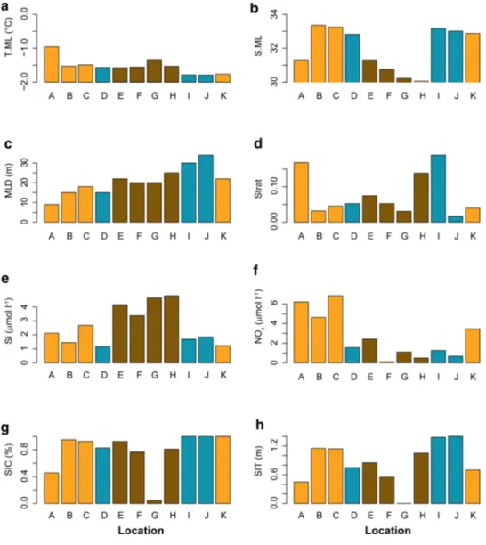
The research area was characterised by mixed layer depths (MLD) between 9 and 34 m, and chlorophyll a concentrations in the mixed layer (Chl.ML) ranged from 0.06 to 0.30 mg m⁻³ (Table 2). Location A was situated at the ice edge and was the only location where water temperatures in the mixed layer (T.ML) were > − 1 °C (Fig. 2a). All other stations were situated within the pack-ice during the early (locations B–D; Fig. 1a), or during the late phase of the sampling period (locations I–K; Fig. 1b). Locations A and E–H were positioned close to large open water areas (Fig. 1b).

They shared low values of salinity in the mixed layer (S.ML) and relatively low values of sea-ice concentration (SIC) and thickness (SIT), indicating an advanced state of sea-ice melt (Fig. 2b, g, h). Locations D–J were characterised by lower nitrate + nitrite concentrations at the depth of the chlorophyll a maximum (NO_x; < 2.5 µmol l⁻¹) than the other locations. In this group, locations E–H showed elevated silicate concentrations at the depth of the chlorophyll a maximum (Si; Fig. 2e). At locations A–C and K, NOx values exceeded 3.5 µmol l⁻¹ (Fig. 2f).

A principle component analysis (PCA) including the environmental parameters NOx, S.ML, SIC, Si and T.ML could explain 99.85% of the first four principle components. The biplot of the first two components (explaining altogether 92.64% of the variance) showed that the most pronounced environmental gradient in the research area followed the variability of S.ML and Si along component axis 1 (Fig. 3). This ‘shelf-ocean’ gradient reflected the transition from locations E–H off the Laptev Sea, characterised by the fresh, silicate-rich waters and decaying sea ice (‘shelf- influenced regime’) to the silicate-poor, more oceanic locations A–D and I–K. (Figs. 2b, e, 3). Crossing this shelf- ocean gradient, an ‘NO_x’ gradient reflected the transition from NOx-poor waters at the shelf-influenced regime (E–H) and a ‘Polar regime’ with low Si values (D, I, J) to NOx-rich waters entering from the Fram Straight at locations A–C and K (‘Atlantic regime’; Figs. 2f, 3). Mean values of Si and NOx were significantly different between the regimes separated by these two interacting gradients (Si: ANOVA, F₂= 23.18, p < 0.001, Tukey HSD: Shelf-influenced versus Atlantic regime p = 0.001/Shelf-influenced versus Polar regime p < 0.001; NOx: ANOVA, F₂= 14.01, p = 0.002, Tukey HSD: Polar versus Atlantic regime p = 0.009/Shelf/

influenced versus Atlantic regime p = 0.003).

(8)

Community structure

General community composition

From the 11 locations considered in this study, we sampled 7 locations for under-ice and epipelagic protists, 9 locations for under-ice metazoans, and 9 locations for epipelagic metazoans (Table 1). In each community, the sampling included locations from all three environmental regimes. In the protist community from under-ice water, OTUs from dinoflagellates ( ~ 40% of total sequences) dominated, with the highest sequence abundances in the Gymnodiniaceae (Gymno- dinium spp., Karlodinium spp. and Gyrodinim spp.). In the epipelagic layer, the share of OTUs from non-dinoflagellate heterotrophic protists was often higher than the share of dinoflagellate OTUs, with the highest sequence abuncances in Ciliophora (Oligotrichea). The under-ice metazoan community comprised both ice-associated and pelagic species. It was numerically dominated by the ice-associated amphipod

Apherusa glacialis, and the pelagic copepods Calanus gla- cialis and C. hyperboreus. The epipelagic metazoan commu- nity was dominated by copepods in numbers and biomass.

By far the most abundant species were C. hyperboreus and Calanus spp. (predominantly C. finmarchicus). Detailed analyses of the taxonomic composition of protist and metazoan communities were provided in David et al. (2015), Ehr- lich (2015) and Hardge et al. (2017a).

Community structure in relation to environmental parameters

In all four communities, the ordination followed gradients of sea-ice influence (SIC, SIT), stratification (MLD, Strat) and shelf influence (S.ML, Si; Table 3). With two excep- tions (under-ice metazoans: location A in Fig. 4c; epipelagic metazoans: location C in Fig. 4d), locations with high sea-ice influence (B–C, I–K) were separated along the SIC/

SIT gradient from those with lower sea-ice influence (D–H;

Fig. 2 Environmental properties at the sampling locations.

Environmental parameters have the same codes as shown in Table 2: T.ML water temperature in the mixed layer (a), S.ML salinity in the mixed layer (b), MLD mixed layer depth (c), Strat stratification index (d), Si Silicate concentration at the depth of the chlorophyll a maximum (e), NOx Nitrate + Nitrite concentration at the depth of the chlorophyll a maximum (f), SIC sea ice concentration (g), SIT ice thickness (h). Capital letters indicate sampling locations from Table 1. The bars are coloured according to environmental regimes identified with the PCA (Fig. 3): brown shelf-influenced regime (Locations E-H);

orange Atlantic regime (Loca- tions A-C, K), turquoise = Polar regime (Locations D, I, J).

(Color figure online)

(9)

Figs. 2, 4). NOx was only important in protist communities (Table 3, Fig. 4a, b).

Trophic structure

Whereas the taxonomic structure of all four communities predominantly reflected the variability of sea-ice influence, stratification and shelf influence (Table 3, Fig. 4), the trophic structure differed predominantly between locations in the

NO_x-rich Atlantic regime and locations in the NO_x-poor Polar and shelf-influenced regimes.

The protist community of the under-ice water was dominated by OTUs of mixotrophic taxa, reflecting the high share of OTUs from dinoflagellates (Hardge et al. 2017a). Loca- tions in NOx-poor waters of the polar and shelf-influenced regimes (D, F and H–J) had a significantly higher share of heterotrophy-associated OTUs than locations of the Atlantic regime (B, K; t test: t_2.24 = 6.32, p < 0.05; Fig. 5a). Within the NOx-poor regimes, locations associated with thicker ice (H–J) had proportionally higher shares of OTUs indica- tive of autotrophic taxa compared to locations with thinner, decaying sea ice (D, F; Figs. 2h, 5a).

In the epipelagic protist community, OTUs of heterotrophs were generally more abundant compared to the protist community sampled in the under-ice layer, reflecting the high share of protozoan sequences in this community (Hardge et al. 2017a). Similar to the under-ice protist community, the proportion of heterotrophic OTUs was higher at the NO_x-poor locations in the Shelf-influenced and Polar regimes (D, F, H–J) than at locations in the Atlantic regime (B, K), but this pattern was not statistically significant (t test: p > 0.05). Rather, the share of OTUs from mixotrophs was significantly lower, and the share of OTUs from autotrophs was significantly higher at NO_x-poor locations compared to locations in the Atlantic regime (t test; mixotrophs:

t_4.42= – 4.58, p < 0.01; autotrophs: t_4.63 = 4.98, p < 0.01;

Fig. 5b).

The under-ice metazoan community was characterized by a high variability in the biomass share of herbivores, ranging from < 30 to > 90% (Fig. 5c). The biomass share of herbivores decreased along the more open and fresher surface water at stations D–G with relatively thin ice (Figs. 1, 2h, 5c). At NOx-poor locations in the shelf-influenced and Polar regimes (D–H), the proportional biomass of herbivores was significantly lower, and proportional biomasses of carnivores was significantly higher compared to locations in the Atlantic regime (A–C, K) (t test: herbivores: t_9.75 = 2.91, p < 0.05; carnivores: t_6.93 = − 2.56, p < 0.05).

Fig. 3 Biplot of a principle component analysis (PCA) of environmental properties in the research area. Capital letters represent sampling locations from Table 1. Letters were colour-coded according to visually identified oceanographic regimes: brown = shelf-influenced regime (Locations E-H); orange = Atlantic regime (Locations A-C, K), turquoise = Polar regime (Locations D, I, J). Blue arrows point into the direction of increasing values of environmental parameters in the ordination. Percentage values in axis annotations indicate proportion of explained variance of the PCA. Environmental parameters (Table 2): NOx Nitrate + Nitrite concentration at the depth of the chlorophyll a maximum, S.ML salinity in the mixed layer, Si Silicate concentration at the depth of the chlorophyll a maximum, SIC sea ice concentration, T.ML temperature in the mixed layer. (Color figure online)

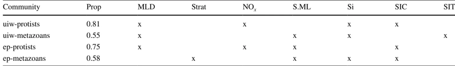
Table 3 Significant (CCA-ANOVA; p < 0.05) combinations of environmental parameters explaining > 50% of the variability in the CCA ordination of protist and metazoan communities at the ice–water

interface and in the epipelagic habitat. In each CCA, the selected significant environmental parameters were indicated by the letter “x”

Habitats: uiw under-ice water, ep pipelagic; Env. parameters: MLD mixed layer depth, NOx = Nitrate + Nitrite concentration at the depth of the chlorophyll a maximum, S.ML salinity in the mixed layer, Si silicate concentration at the depth of the chlorophyll a maximum, SIC sea ice concentration, Strat stratification index, SIT ice thickness. Statistics: prop. = proportional contribution of eigenvalues to constraints

Community Prop MLD Strat NOx S.ML Si SIC SIT

uiw-protists 0.81 x x x x

uiw-metazoans 0.55 x x x x

ep-protists 0.75 x x x x

ep-metazoans 0.58 x x x x

(10)

In the epipelagic metazoan community, the variability of the biomass share of herbivores versus carnivores showed a similar pattern compared to the under-ice protist and under- ice metazoan communities (Fig. 5 a, b, d). Accordingly, at NOx-poor locations in the shelf-influenced and Polar regimes (D–F, H–J), the proportional biomass of herbivores was significantly lower, and the proportional biomass of omnivores and carnivores was significantly higher compared to locations in the Atlantic regime (B, C, K) (t test; herbivores:

t_3.06 = 4.10, p < 0.05; omnivores: t_3.19 = − 3.45, p < 0.05;

carnivores: t_3.06 = − 3.85, p < 0.05).

To more accurately investigate the relationship of trophic structure with the variability of environmental parameters interacting with each other, we used GLMs to analyse the combined effect of up to two environmental parameters on the relative share of each trophic group from

each community in each habitat. In 10 of the 12 models, the selection procedure resulted in ‘best’ models with significant effects (p < 0.05) (Table 4). In under-ice communities, the proportional contribution of each trophic group was associated with different environmental parameters.

For the under-ice protist community, the selected GLMs indicated that temperature and turbidity of the mixed layer had a positive effect on the share of autotrophs, while heterotrophs were negatively related to NOx values and positively related to chlorophyll a concentrations in sea ice. The share of mixotrophs was negatively related to ice thickness (Table 4). In under-ice metazoan models, S.ML was the only environmental parameter related to the two trophic groups to which a GLM could be fitted. S.ML had a positive effect on the share of herbivores, and a negative effect on the share of carnivores (Table 4). Because this

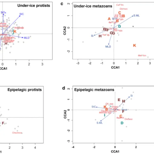
Fig. 4 Biplots from a canonical correspondence analysis (CCA) of under-ice protist (a), epipelagic protist (b), under-ice metazoan (c) and epipelagic metazoan (d) communities in relation to environmental gradients. Capital letters in biplots indicate sampling locations (Table 1). Letters were colour-coded according to oceanographic regimes (Fig. 3): brown = shelf-influenced regime (Locations E-H);

orange = Atlantic regime (Locations A-C, K), turquoise = Polar regime (Locations D, I, J). Blue arrows point into the direction of increasing values of environmental parameters in the ordination. Grey

dots indicate the position of individual protist OTUs and metazoan taxa in the ordination. The corresponding taxonomic information is provided in the Online Resource (ESM1, ESM2). Environmental parameters (Table 2): MLD mixed layer depth, NOx Nitrate + Nitrite concentration at the depth of the chlorophyll a maximum, S.ML salinity in the mixed layer, Si Silicate concentration at the depth of the chlorophyll a maximum, SIC sea ice concentration, Strat = stratifica- tion index, SIT = ice thickness. (Color figure online)

(11)

community was not sampled at locations I and J, however, the variability of S.ML largely coincided with the variability of NO_x in this dataset.

In the epipelagic layer, NOx had a significant effect in all five GLMs fitted (Table 4). The two trophic groups of protist communities to which a GLM could be fitted were both associated with the chlorophyll a concentration in the mixed layer (Chl.ML) and NOx, with a positive effect in the model of mixotrophs, and a negative effect of these parameters in the model of heterotrophs (Table 4). In epipelagic metazoan models, NO_x was the only environmental parameter significantly related to all three trophic groups, with a positive

effect in the model of herbivores and negative effects in the models of omnivores and carnivores (Table 4).

Discussion

Structure of the environment

In summer 2012, the Eurasian Basin was characterised by extremely low sea-ice coverage, super-imposed on environmental gradients determined by the large-scale hydrography of the Arctic Ocean. Sea-ice-conditions changed from a

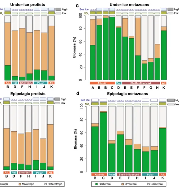
Fig. 5 Trophic structure of under-ice protist (a), epipelagic protist (b), under-ice metazoan (c) and epipelagic metazoan (d) communities. The heights of the coloured sections in the bars indicate the proportional abundances of operational taxonomic units (OTU) in protist communities and biomass shares in metazoan communities. Capital letters indicate sampling locations from Table 1. Duplicate letters indicate repeated sampling at the same location (Table 1). Symbols

above the bars indicate either ‘high’ or ‘low’ conditions of sea ice and NOx, respectively, based on the data shown in Fig. 2. The coloured horizontal blocks below the bars indicate the 3 hydrographical regimes of the research area: Atlantic regime (orange), shelf-influenced regime (brown), and Polar regime (turquoise). (Color figure online)

(12)

nearly closed sea-ice cover at the beginning of our sampling in the Nansen Basin (Fig. 1a), through an opening area of rapid sea-ice melt in the Laptev Sea sector south of 86°N, and back into freezing conditions at higher latitudes and towards the end of the survey in late September (Fig. 1b).

Sea-ice concentration (SIC) was a significant, but not very pronounced contributor to our PCA (Fig. 3). However, the vast ice-free zone in the Laptev Sea sector may have been under-represented by our satellite-derived sea-ice concentration values from the relatively small areas around our ice- covered sampling stations (Fig. 1b). In the epipelagic layer, the most pronounced environmental gradient was created by the silicate concentration in the chlorophyll a maximum (Si). The high-silicate concentrations at locations E–H in the shelf-influenced regime reflected the influence of Laptev Sea water carrying high amounts of silicate originating from the Lena delta inflow, as compared to the low Si values at all other locations (Fig. 2; Bauch et al. 2014; Bluhm et al.

2015). The salinity in the mixed layer (S.ML) varied largely in the opposite direction of the silicate gradient (Figs. 2, 3). Crossing this silicate/salinity gradient, Nitrate + Nitrite concentrations in the chlorophyll a maximum (NOx) changed from high values in the Atlantic regime (locations A–C, K) to low values in the shelf-influenced and Polar regime (locations D–J). This large-scale NOx-gradient was consistent

with the known pattern of NOx distribution in the Arctic Ocean during summer (Codispoti et al. 2013; Bluhm et al.

2015): In the Eurasian Basin, nitrate is predominantly advected by the Atlantic water inflow through the Fram Strait and across the Barents Sea, and transported along the Eurasian shelf break, where our sampling locations A–C and K were situated. After reaching the Laptev Sea sector, surface waters are depleted of NO_x and recirculated across the Eurasian Basin towards the Fram Strait, passing the posi- tions of our NOx-poor sampling locations D–J (Kattner et al.

1999; Rudels et al. 2013; Bluhm et al. 2015).

Taxonomic community structure

Gradients of sea-ice influence (SIC, SIT), stratification of the water column (MLD, Strat) and shelf influence (S.ML, Si) were common drivers of the community structure in all four communities (Table 3). The effects of these drivers on community composition cannot be entirely disentangled from each other, because the directions of their gradients often overlapped in the CCA ordination (Fig. 4). However, the general pattern in the four CCA ordinations showed that locations associated with low sea-ice influence were separated from stations with high sea-ice influence along gradients of sea-ice properties (SIC, SIT; Fig. 4). Sea ice

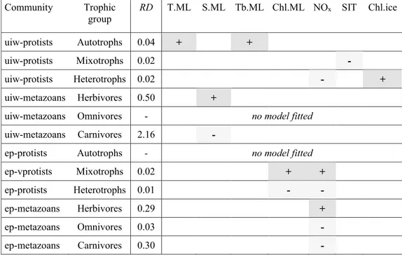
Table 4 Summary of ‘best’ Generalized Linear Models (GLM) of the relationship between the proportional contribution of trophic groups and environmental parameters in protist and metazoan communities in the under-ice layer and the epipelagic layer

Community Trophic

group RD T.ML S.ML Tb.ML Chl.ML NOx SIT Chl.ice

uiw-protists Autotrophs 0.04 + +

uiw-protists Mixotrophs 0.02 -

uiw-protists Heterotrophs 0.02 - +

uiw-metazoans Herbivores 0.50 +

uiw-metazoans Omnivores - no model fitted

uiw-metazoans Carnivores 2.16 -

ep-protists Autotrophs - no model fitted

ep-vprotists Mixotrophs 0.02 + +

ep-protists Heterotrophs 0.01 - -

ep-metazoans Herbivores 0.29 +

ep-metazoans Omnivores 0.03 -

ep-metazoans Carnivores 0.30 -

The directional effect of each parameter on the response variable is indicated by “+” signs (dark shading) and “−” signs (light shading)

Habitats: ep epipelagic, uiw under-ice water; Environmental parameters: Chl.ice chlorophyll a concentration in sea ice, Chl.ML chlorophyll a concentration in the mixed layer, NO_x nitrate + nitrite concentration at the depth of the chlorophyll a maximum, S.ML salinity in the mixed layer, SIT ice thickness, Tb.ML turbidity in the mixed layer, T.ML temperature in the mixed layer; statistics: RD residual deviance of GLM

Significance of model terms: *p < 0.05, **0.05 < p < 0.001; ***p < 0.001

(13)

influences protist communities in the water column primarily by limiting light intrusion, affecting photo-autotrophic growth (Sakshaug 2004). Other important factors influencing protist community composition are limitation of nutrient supply from deeper water layers due to enhanced stratification under melting sea ice (Fujiwara et al. 2014), and exchange between the water column and in-ice communities through physical processes and active migration (Hardge et al. 2017a). The observed relationship between protist community structure and sea-ice properties contrasts an extensive analysis by Ardyna et al.

(2011) in the Canadian Arctic, which found that sea ice- conditions played only a minor role. The work of Ardyna et al. (2011) was conducted on the Pacific-influenced shelf of the Canadian Archipelago, whereas our study was conducted in the deep Eurasian Basin. Apart from these bio- geographical differences, it is possible that the range of mean sea-ice concentrations (2–23%) observed by Ardyna et al. (2011) in late summer was too limited to significantly affect protist communities through shading, stratification, or organism exchange. In agreement with Ardyna et al.

(2011), the structure of protist communities in our study was also significantly related to NOx gradients. In metazoan communities, however, a significant influence of NO_x was not observed in our dataset (Table 3).

In the under-ice metazoan community, a strong response to sea-ice influence was expected due to the high proportional abundance of sea ice-associated (sympagic) amphi- pods, e.g. Apherusa glacialis and Onisimus glacialis (Hop et al. 2000; Poltermann et al. 2000; Gradinger and Bluhm 2004; Bluhm et al. 2010). David et al. (2015) observed that the under-ice metazoan community structure differed between a densely ice-covered ‘Nansen Basin regime’

(corresponding to the Atlantic regime in the present study), and a more open ‘Amundsen Basin regime’ (the Shelf-influenced regime in the present study) in summer 2012. Our observation that sea-ice concentration was an important factor structuring the epipelagic metazoan community (Table 3) is in agreement with a multi-annual study in the Western Arctic Ocean finding that the contribution of sea-ice concentration to the variability in zooplankton community structure ranked highest together with bathymetry among numerous investigated environmental parameters (Hunt et al. 2014). In the epipelagic metazoan community ordination, crossing gradients of sea-ice properties (SIC) and shelf influence (S.ML, Si) indicated that, in combination with sea-ice influence, the epipelagic metazoan community structure responded to shelf influence (Fig. 4d). Most high-Arctic zooplankton studies focused on horizontal and vertical differences in community structure in relation to large, physically defined water masses and bathymetrically defined habitats (e.g., Mumm et al.

1998; Kosobokova and Hirche 2000; Wassmann et al.

2015). The shelf-influence gradient (S.ML/Si) of our CCA resembled such a hydrographical pattern (Fig. 4d).

In the Eurasian Basin, plankton communities are strongly influenced by Atlantic species advected through the Fram Strait and the Barents Sea (Wassmann et al.

2015). While in our research area, the advection of Atlan- tic species is tied to the distribution of Atlantic water flow- ing eastward along the continental slope at depths below 100 m, surface waters of Polar origin are associated with the westward Transpolar Drift transporting sea ice from Siberia towards the Fram Strait. Advection of Polar species with surface waters thus probably contributed partly to the sea ice-associated gradient in protist and metazoan community structure. The sea ice itself may have advected species from the Siberian shelf, as has been found for sea- ice protists by Hardge et al. (2017a), and for polar cod Boreogadus saida by David et al. (2016). Besides the physical properties of sea ice, the presence of ice algae may have attracted certain zooplankton and sympagic species, and contributed to a sea-ice-driven trend in under- ice and epipelagic metazoan community composition.

Ice algae were an important carbon source of abundant metazoan species in summer 2012, accounting for up to about 50% of the carbon demand in the pelagic copepods Calanus spp., and over 90% in the sympagic amphipod Apherusa glacialis (Kohlbach et al. 2016).

Hydrographical structures, sea-ice properties and advection patterns were major drivers of community composition. Several of these drivers were intrinsically linked to seasonal changes in both habitats, impeding a clear dis- entanglement of seasonal change and environmental drivers. In 2012, the sampling period extended over 9 weeks from summer to the onset of winter (Table 1). Seasonal changes were indicated by decreasing temperatures in the mixed layer (T.ML), increasing mixed layer depth (MLD) and high sea-ice concentrations (SIC) towards the end of the sampling period (Fig. 2). In the under-ice habitat, seasonal processes, such as the increased exchange of protist communities between water column and sea ice during the onset of freezing (Hardge et al. 2017b) and the seasonal downward migration of copepods (David et al. 2015) probably influenced community structure at locations I–K (Fig. 4a, c). In the epipelagic habitat, seasonal change of community composition appeared less pronounced, as the hydrographically similar earliest and latest locations B and K grouped closely together in the CCA (Fig. 4b, d). This indicates that seasonal change of community composition was most pronounced at the ice–water interface due to the more extreme physical changes at the surface, e.g. from melting conditions to freeze-up.

(14)

Trophic community structure

Variability of sea-ice properties was an important driver of the taxonomic community structure in both protists and metazoans (Table 3, Fig. 4). This pattern, however, was not mirrored in the trophic structure of the communities. In all four communities, a stronger dominance of the most heterotrophic trophic group (protists: heterotrophs; metazoans:

carnivores) was associated with sampling locations of the shelf-influenced and Polar regimes with low nitrate + nitrite concentrations (NOx) (Fig. 5). Conversely, the dominance of the most heterotrophic trophic group was negatively related with NO_x in both protist communities and in epipelagic metazoans (Table 4). When primary production is limited by nutrient depletion, heterotrophic processes can be expected to increase in relative importance, because autotrophs and their herbivorous grazers cannot realise their full growth potential relative to their heterotrophic competitors and predators. Basedow et al. (2010) explained an increase in mean trophic levels of the zooplankton community from a bloom- to a post-bloom situation in the Barents Sea by a switch from a dominance of small herbivorous zooplankton to a dominance of carnivorous zooplankton, combined with a change in the diet of omnivorous grazers, such as Calanus spp. Our results show that similar processes take place in the central Arctic Ocean. A dominance of heterotrophic processes has been linked with nutrient limitation in several ecosystems of the Western Arctic Ocean bordering the Canada Basin, due to either hydrographical structures (e.g.

shelf versus basin), or seasonal succession (Cota et al. 1996;

Levinsen et al. 1999; Nielsen and Hansen 1999; Forest et al.

2014). The Canada Basin is a mostly oligotrophic environment, because nutrient input through the Bering Strait and by riverine input is used up on the shelf (Tremblay et al.

2015). In contrast, the Eurasian Basin receives substantial nutrient input through the Fram Strait, which is redistributed by the surface currents, leading to strong gradients. Because of these more intensive nutrient dynamics in the Eurasian Basin, changes in the trophic structure of the ecosystem due to changing nutrient distribution can be expected to be more pronounced. Therefore, we consider the Eurasian Basin a well-suited model system to study the interacting effects of sea-ice distribution and nutrient availability on the ecosystem of the central Arctic Ocean.

Our analysis of trophic structure faces several caveats that are founded in the quantification of protist community structure by OTUs rather than abundances or biomass, and in limited knowledge about the trophic ecology of various protist and metazoan taxa. Generally, it is difficult to relate sequence abundances of protists to cell number or biomass, because the number of target gene copies varies between protist species (Prokopowich et al. 2003; Zhu et al. 2005;

Godhe et al. 2008; Egge et al. 2013). A microscopic analysis

of two subsurface water samples (locations C and H; Online Resource ESM3) found that diatoms constituted 3–5% of the protist biomass, which was in agreement with the low share of diatom sequences and biomass in our study region (Roca-Martí et al. 2016; Hardge et al. 2017b). Microscopic analysis further confirmed the dominance of dinoflagellates in OTU abundances (Hardge et al. 2017b), but indicated that the relative biomass of ciliates could have been higher by a factor of 2–3 compared to the relative OTU abundance.

Furthermore, we likely underestimated the abundance of haptophytes due to insufficient coverage of the 18S rRNA gene primer set used (Balzano et al. 2012; Bradley et al.

2016). In spite of these limitations, we assume that relative differences in OTU abundance patterns between environmental regimes realistically reflect the intrinsic variability of the system investigated here, because the potential bias of relative OTU abundances compared to relative abundance or biomass affected all samples equally. In our approach to analyse the trophic structure of the two protist communities we classified dinoflagellates as mixotrophs, because many dinoflagellates can switch between a photo-autotrophic and a heterotrophic mode of life. Dinoflagellates in autotrophic mode, however, are rare in Arctic oceanic ecosystems during late summer (Levinsen et al. 1999; Nielsen and Hansen 1999), and they constituted less than 0.1% of the dinoflagellate biomass in the microscopic analysis (Online Resource ESM3). Likewise, we classified Calanus copepods as herbivores, although they can prey substantially on microzooplankton (Ohman and Runge 1994; Levinsen et al.

2000; Campbell et al. 2009). Bulk stable isotope data from Calanus spp. from our sampling campaign showed that mean δ¹⁵N values ranged between 2.7–3.5 and 3.0–3.8‰

above the trophic baselines of ice algae and phytoplankton in C. glacialis and C. hyperboreus, respectively (Kohlbach et al. 2016). Assuming a mean δ¹⁵N enrichment of 3.4‰

per trophic level (Minagawa and Wada 1984), the two most abundant Calanus copepods in our study would be considered herbivores. Yet, even a conservative approach consider- ing Calanus spp. as omnivores would not change the general pattern of an increased dominance of carnivores in locations with low NO_x values compared to locations with high NO_x values (Fig. 5c, d).

The ecosystem investigated in this study has been characterised as a system with low primary productivity (Fernán- dez-Méndez et al. 2015), supporting a food web that was nonetheless capable of sustaining a significant population of polar cod Boreogadus saida (David et al. 2016; Kohlbach et al. 2017). In high-Arctic ecosystems, primary productivity is usually limited to a short period in springtime, from the onset of light intrusion through sea-ice, until the available nutrient stocks are consumed to depletion (e.g. Hill et al.

2013). This springtime bloom starts with ice algae and continues in the water column under thinning sea ice, and in