Playing with Boolean Blocks, Part II:
Constraint Satisfaction Problems
1Elmar B¨ ohler
2, Nadia Creignou
3, Steffen Reith
4, and Heribert Vollmer
5Introduction
In the previous column we played with Boolean functions as “building blocks” in the construction of switching circuits. In the meantime we got to know a child, having a great collection of essentially the same blocks. However, during her construction process she uses the blocks in a completely different way than we do: she uses Boolean functions not to build switching circuits but to formulate queries to a database. Nevertheless our games are closely related and there is a bridge to connect them. Therefore we will tell you more about the new game and the connection in this issue.
Every Boolean function trivially defines a Boolean relation. The relation is the set of all tuples, for which the function-value is 1. For instance the 2-ary Boolean or-function defines the relation {(0,1),(1,0),(1,1)}. Instead of asking whether a function maps an input-tuple to 1, we now ask whether it belongs to the relation. That means that eachn-ary relation is a constraint on the set of all n-tuples. This leads us to the rich field of “constraint satisfaction”, which has numerous appli- cations in computer science (database querying, circuit design, network optimization, scheduling, logic programming), artificial intelligence (planning, belief maintenance, languages for knowledge based systems), and computational linguistics (processing of natural languages) [Kol03].
In the world of Boolean constraint satisfaction we start with a box that contains Boolean constraints. There is only a finite number of different constraint types in the box, but of each type we have an infinite number of “copies”. Now we want to combine them in order to get new constraints. First fix a set of constraints. We build a new constraint as follows: Make a list of constraints which are taken out of the fixed set. Check for each suitable Boolean tuple whether it fulfills all constraints of the list. If this is the case the tuple fulfills the newly built constraint. What does that mean? This means that we simply connect the constraints using “and”. In this context one important problem is to check whether a collection of constraints does not define the empty relation. Suppose we have built a constraint as explained out of a finite set of Boolean relations S (such a constraint is considered as a formula in generalized conjunctive normal form, a so called S-formula or CNF(S)), then this problem is known as generalized satisfiability problem, denoted by SAT(S), and was first investigated by Thomas Schaefer in 1978. Here we are interested in the complexity of SAT(S). It turns out that its complexity can be characterized by the set of so called closure properties ofS, which is the set of functionsf of aritymsuch that if we applyf coordinate- wise to m vectors of any relation R from S, then the result is again in R. This correspondence is obtained through a generalization of Galois theory. Since this set of closure properties—a set of Boolean functions—is a clone, we have now a connection between the complexity of Boolean
1Elmar B¨c ohler, Nadia Creignou, Steffen Reith, and Heribert Vollmer, 2003. Supported in part by ´EGIDE 05835SH, DAAD D/0205776 and DFG VO 630/5-1.
2Theoretische Informatik, Fachbereich Mathematik und Informatik, Universit¨at W¨urzburg, Am Hubland, 97072 W¨urzburg, Germany,boehler@informatik.uni-wuerzburg.de.
3Laboratoire d’informatique fondamentale, Facult´e des sciences de Luminy, Universit´e de la M´editerran´ee, 163 avenue de Luminy, 13288 Marseille cedex 9, France,creignou@lidil.univ-mrs.fr.
4Lengfelderstr. 35b, 97078 W¨urzburg, Germany,streit@streit.cc.
5Theoretische Informatik, Fachbereich Informatik, Universit¨at Hannover, Appelstraße 4, 30167 Hannover, Germany,vollmer@thi.uni-hannover.de.
constraint satisfaction problems and the clone theory presented in the first part of this column.
Therefore we will show that Post’s lattice can also be a very useful tool for studying the complexity of Boolean constraint satisfaction problems.
1 Closed Classes of Boolean Constraints
The study of constraint satisfaction problems (CSPs) leads to a powerful general framework in which a variety of combinatorial problems can be expressed. The aim in a constraint satisfaction problem is to find an assignment of values to the variables subject to specified constraints. This framework is used in a many research areas in computer science. Here and in the next section we will have a look at the complexity of Boolean constraint satisfaction problems and show that it depends solely on the sort of constraint relations one is allowed to use in the instance.
1.1 Boolean Constraints
Throughout the paper we use the standard correspondence between propositional formulas (predi- cates) and relations: a relation consists of all tuples of values for which the corresponding formula holds. We will use the same symbol for a predicate and its corresponding relation, since the meaning will always be clear from the context, and we will say that the formularepresents the relation.
An n-aryBoolean constraint relation Ris a Boolean relation of arityn, i.e.,R⊆ {0,1}n. LetV be a set of variables, then aconstraint application (or simply, aconstraint)Cis an application ofR to ann-tuple of (not necessarily distinct) variables fromV, i.e.,C=R(x1, . . . , xn). An assignment I:V → {0,1}satisfies the constraint R(x1, . . . , xn) if and only if (I(x1), . . . , I(xn))∈R.
Example 1.1. For 0 ≤ l ≤ k, if Rork,l is the k-ary relation Rork,l = {0,1}k \ {1l0k−l}, then Rork,l(x1, . . . , xk) = (¯x1∨. . .∨x¯l∨xl+1∨. . .∨xk).
If RNAE and ROne-Exactly are the ternary relations RNAE = {0,1}3 \ {(0,0,0),(1,1,1)} and ROne-Exactly ={(1,0,0),(0,1,0),(0,0,1)}, then the constraint RNAE(x, y, z) is satisfied if and only if not all the three variables are assigned the same value and the constraint ROne-Exactly(x, y, z) is satisfied if and only if exactly one of x,y and z is assigned true.
Example 1.2. The equivalence relation is the binary relation given by Eq ={(0,0),(1,1)}.
Throughout the text we will refer to different types of Boolean constraint relations, following the terminology of Schaefer [Sch78].
– A Boolean relationR is0-valid (1-valid , resp.) if (0, . . . ,0)∈R ((1, . . . ,1)∈R, resp.).
– A Boolean relation R is Horn (anti-Horn, resp.) if R can be represented by a conjunctive normal form (CNF) formula having at most one unnegated (negated, resp.) variable in any conjunct.
– A Boolean relationR isbijunctive if it can be represented by a CNF formula having at most two variables in each conjunct.
– A Boolean relation R is affine if it can be represented by a conjunction of linear functions, i.e., a CNF formula with⊕-clauses (XOR-CNF).
– A Boolean relationR iscomplementive if for all (α1, . . . , αn)∈R also (α1, . . . , αn)∈R.
A set S of Boolean relations is called 0-valid (1-valid, Horn, anti-Horn, affine, bijunctive, com- plementive, resp.) if every relation in S is 0-valid (1-valid, Horn, anti-Horn, affine, bijunctive, complementive, resp.). A constraint set S is called Schaefer, if S is Horn, anti-Horn, affine, or bijunctive.
There are easy criteria to determine if a given relation is Horn, anti-Horn, bijunctive, or affine.
– A relation R is Horn, if and only if for all vectors x, y ∈ R, the vector obtained by taking coordinate-wise the logical conjunction, in symbols: x∧y, is in R [DP92], see also [CKS01, Lemma 4.8]. Similarly, the property anti-Horn is characterized by coordinate-wise disjunction.
– A relation R is bijunctive, if and only if for all vectors x, y, z ∈ R, the vector obtained by taking coordinate-wise majority (i.e., the ith coordinate is set to 1 if and only if in at least two ofx, y, z theith coordinate is 1) is inR [Sch78], see also [CKS01, Lemma 4.9].
– A relationR is affine, if and only if for all vectors x, y, z∈R, the vector obtained by taking coordinate-wise logical exclusive-or (x⊕y⊕z) is inR[Sch78, CH96], see also [CKS01, Lemma 4.10].
Thus, each of these criteria is given in form of a closure property of the set of all vectors in R, and each involves an operation performed on these vectors coordinate-wise.
We prove the characterization of Horn: Suppose R is Horn. Consider a clause C in the repre- sentation ofR by a Horn formula, and two assignmentsI1, I2 that satisfyC. If one ofI1, I2 satisfies one of the negative literals in C, then the same literal is satisfied in I1∧I2. If bothI1, I2 satisfy the positive literal in C, then of course this literal is also satisfied by I1∧I2. Thus we see that if x, y∈R, thenx∧y∈R.
For the converse, let us first introduce a definition. A subset of literals defined over the variables ofRis amaxterm ofRif setting each of the literals false determines the predicate to be false and it is a minimal such collection. IfR is not Horn, then one can prove thatR has at least one maxterm that is not Horn [CKS01, Lemma 4.7, page 29]. Suppose that this maxterm, C, contains at least two positive literals, say xi and xj. Let I1 be the assignment that satisfies variable xi plus those variables occurring negated inC and falsifies all other variables, and letI2 be the assignment that satisfiesxj plus those variables occurring negated in C and falsifies all other variables. ThenI1, I2 satisfyC, but the coordinate-wise conjunction I1∧I2 does not satisfy C. Hence we found vectors x, y∈R with the property x∧y6∈R.
The proof of the characterization of anti-Horn is analogous, and the proof of the characterization of bijunctive is very similar. The proof for affine constraints rests on a classical characterization of affine subspaces in linear algebra and can be found, e.g., in [CKS01, p. 30].
1.2 Assembling Boolean Constraints: Generalized Propositional Formulas and Con- junctive Queries
We will now consider formulas that are conjunctions of constraints, where the constraints are given by Boolean relations. LetS be a non-empty finite set of Boolean relations. Then S-formulas are conjunctive propositional formulas consisting of clauses built by using relations fromS applied to arbitrary variables. Formally, let S be a set of Boolean relations and V be a set of variables. An S-formula F (overV) is a finite conjunction of clausesF =C1∧. . .∧Cp, where each clauseCi is a constraint application of some constraint relationR∈S. IfF =C1∧. . .∧Cp is such a formula over V and I is an assignment with respect to V, then I |=F ifI satisfies all clauses Ci. By CNF(S) we denote the set of all S-formulas as just defined.
Schaefer in his seminal paper was interested in a classification of the complexity of satisfiability ofS-formulas. In order to obtain such a result, so called conjunctive queries turn out to be useful.
Conjunctive queries play an important role in database theory (they are equivalent to select-join- project queries in relational algebra) and thus are also of interest in their own right.
Given a set S of Boolean relations, let us denote by COQ(S) the set of all formulas of the form
∃x1∃x2. . .∃xkφ(x1, . . . , xk, y1, . . . , yl), whereφ is a CNF(S); these formulas are called conjunctive queries (overS)[KV00]. In other words, a relation can be represented by a conjunctive query if and only if it is a projection of a relation that can be represented by anS-formula [JCG99, Definition 4, Lemma 1, and Notation 3].
Intuitively constraints using relations from COQ(S) are those which can be “simulated” by constraints using relations in S. We remark that in Schaefer’s terminology, COQ(S) was denoted by Rep(S).
1.3 Closure Properties of Constraints: a Little Bit of Galois Theory
As we have already seen, there are easy criteria to determine whether a given relation is Horn, anti-Horn, bijunctive or affine. All these criteria work essentially in the same way: If you apply a special Boolean function f coordinate-wise on some of the elements of the relation R, then the result of this application must be again an element in R. Moreover we have some more subtle common properties. Recall the test for affine. A relationR is affine if and only if it is closed under coordinate-wise application of x1⊕x2⊕x3. Since we have no particular order of the elements of R, it is clear thatR is affine if and only if we can do the same test withxπ(1)⊕xπ(2)⊕xπ(3) for any permutation π:{1,2,3} → {1,2,3}. Note that this argument does not rest on the commutativity of⊕and it will also work for other tests of this kind. Now we identify variables inx1⊕x2⊕x3to get the 2-ary function f0(x1, x2) = f(x1, x2, x2). If the relation is affine and we apply the function f0 on some elements ofR we will surely obtain an element ofR, which shows thatf0 also “preserves”
the relation R. Finally take the function f00(x1, x2, x3, x4, x5) = x1 ⊕x2⊕(x3⊕x4 ⊕x5), which is obtained by the operation of substitution from the original function x⊕y⊕z. Clearly we get another element of R if we take five elements fromR and applyf00 coordinate-wise on them. We thus see that the set of functions that preserve R forms a clone. In fact, this holds for arbitrary relationsR. So there is a deeper connection between clones (defined in part I) and relations.
In the following we will see that a generalized Galois theory is the connection we are looking for. The roots of Galois theory were invented by Evariste Galois to find a solution for the classical problem to solve a given polynomial equation by radicals. He was able to give a recursive criterion for solvability in this sense. Additionally his results show that polynomial equations having a degree more than 4 in general cannot be solved with radicals. The modern presentation of this beautiful result establishes a bijection between two worlds: The set of certain extension fields of the field of coefficients and the set of automorphism-groups of this extension field (see e.g. [Art98]).
In the original setting, Galois asked which permutations of zeroes of a polynomial preserve all algebraic dependence relations between these zeroes. (These dependencies are given in the form of polynomial equations, for instance: The square of the first zero is equal to the second zero plus 2, that is: the square of the first zero minus the second zero minus 2 equals 0.) Let Gbe the set of algebraic dependence relations of the zeroes of a polynomial equation. Galois defined a group of permutations—the Galois group—that preserve these relations as follows: A permutationπbelongs to the Galois group if and only if for allh∈G, ifh(ζ1, . . . , ζn) = 0, thenh(ζπ(1), . . . ζπ(n)) = 0, where ζ1, . . . , ζn are the zeroes of the given polynomial equation. Intuitively, if the set of dependencies is “big”, then the number of permutations in the Galois group is “small”, and vice versa. This
matches with the abstract definition of a Galois correspondence given next.
We say that two mappings α:A→B and β:B→A form aGalois correspondence (cf. [PK79, A5.1], [Pip97, Sect. 1.2.3]) between the orders (A,A) and (B,B) if the following properties hold:
1. For alla, b∈A such thataAb, we have α(b)B α(a).
2. For allc, d∈B such thatcB d, we have β(d)Aβ(c).
3. For alla∈A,b∈B we haveaAβ(α(a)) andbB α(β(b)).
With this definition it is not hard to show thatλ1:A→As.t.λ1(a) =β(α(a)) andλ2:B →B s.t.λ2(b) =α(β(b)) are closure-operators [PK79]. (Here, a closure operator in an order (A,A) is a function f:A→A such thataAf(a), ifaAbthenf(a)Af(b), andf(a) =f(f(a)).)
To be able to use this abstract definition in our context of Boolean functions and constraints, we introduce the central notion of aclosure property of a Boolean relation (see, e.g., [JC95, Pip97, Dal00]). As we will see shortly this notion provides an algebraic characterization of COQ(S). Let R be a Boolean relation of arity n and let f be a Boolean function of arity m. For f to be a closure property ofRwe require that if we applyf coordinate-wise tomvectors inR, the obtained vector is again in R; see Fig. 1. More formally, we say that R is closed under f (or f preserves
f( f( f( f(
x1 = 0 1 1 · · · 0 x2 = 1 1 0 · · · 1 ... ... ... ... ... xm = 1)= 1)= 0)= · · · 1)= z = 0 1 0 · · · 0
Figure 1: Ifx1, . . . , xm are in R, then zmust be in R.
R, or f is a polymorphism of R, or R is an invariant of f), if for all x1, . . . , xm ∈ R, where xi = (xi[1], xi[2], . . . , xi[n]), we have
f x1[1],· · · , xm[1]
, f x1[2],· · · , xm[2]
, . . . , f x1[n],· · ·, xm[n]
∈R.
Example 1.3. The set of all Horn relations (of all affine relations, resp.) is the set of all relations that are preserved by the logical conjunction (by the function x⊕y⊕z, resp.).
Let us denote the set of all polymorphisms ofRby Pol(R), and for a setS of Boolean relations, we define Pol(S) to be the set of Boolean functions that are polymorphisms of every relation in S. Then, as in the case of Galois’ algebraic dependencies, if S is “big” then the number of closure properties of S is “small”, and vice versa.
Generalizing the observations we made for affine relationsR in the first paragraph of Sect. 1.3, we see that for every set S, Pol(S) is a clone. (This holds since immediately by definition, Pol(S) is closed under introduction of fictive variables, permutation and identification of variables and substitution, and moreover, contains the projection functions.) Conversely, ifB is a set of Boolean functions, then Inv(B) is defined to be the set of all relations which are preserved by the functions
in B, i.e., the set of relations that are invariants of all functions in B. It turns out that sets Inv(B) have particular common properties: They contain the equivalence relation, and each such set is closed under Cartesian product, projection and identification of variables (see, e.g., [JCG99, Lemma 1]). More generally, for a setSof Boolean relations lethSidenote the closure ofSplus the equivalence relation under the mentioned operations. We say thathSiis theco-clone generated by S (see [Dal00, page 81], [Pip97, Sect. 1.7]). Hence, for every set of Boolean functions B, Inv(B) is a co-clone.
Example 1.4. Horn relations, as well as affine relations, form a co-clone.
Hence Inv and Pol play the role of the functions α and β, resp., in the abstract definition of a Galois correspondence, when we identify the lattice of sets Boolean functions withAand the lattice of sets of Boolean relations with B. A basic introduction to this correspondence can be found in [Pip97, P¨os01] and a comprehensive study in [PK79].
Interestingly, the closure operators λ1 and λ2 from the general setting of a Galois correspon- dence, i.e., in our case the functions Inv(Pol(·)) and Pol(Inv(·)), turn out to coincide with the co-clone- and clone-closure:
Theorem 1.5 ([Gei68, BKKR69],[PK79, Folgerung 1.2.4]). Let S be a set of Boolean rela- tions and B be a set of Boolean functions.
– Inv(Pol(S)) =hSi – Pol(Inv(B)) = [B]
Example 1.6. Consider the constraint ROne-Exactly defined in Example 1.1. The set of polymor- phisms Pol({ROne-Exactly}) is a clone. It contains neither any constant operation nor the negation operation nor the disjunction nor the conjunction nor the majority operation nor the ternary exclusive-or operation. Therefore, looking at Post’s lattice and at the basis of the classes, we see that Pol({ROne-Exactly}) = I2, i.e., consists only of all projections. Thus, Inv(Pol({ROne-Exactly}) consists of all Boolean relations, and then so does h{ROne-Exactly}iby Theorem 1.5.
In the first part of this complexity theory column we have characterized the set of all functions that can be computed by a B-circuit as the closure of B under superposition: CIRC(B) = [B].
Analogously, if we want to know what Boolean relations can be expressed by conjunctive queries over S∪ {Eq} it suffices to look at the closure of the Boolean relations (together with the equivalence relation), S ∪ {Eq}, under Cartesian product, projection and identification of variables. More formally (see [JCG99, Theorem 2], [Dal00, Theorem 20, p. 98]):
Proposition 1.7. For every set S of Boolean relations, COQ(S∪ {Eq}) =hSi.
Proof. The relation associated with a conjunctive query Φ overS∪{Eq}is the projection (existential quantification) of the conjunction of relations occurring in Φ. Thus it is easy to see that COQ(S∪ {Eq}) ⊆ hSi.Conversely, S ⊆COQ(S∪ {Eq}). Now it is easy to check that COQ(S∪ {Eq}) is a co-clone, therefore we have also hSi ⊆COQ(S∪ {Eq}),thus proving the equality.
1.4 The Lattice of Co-clones
As already mentioned in the first part of this column, the set of all clones form a lattice. Because we want to connect clones and co-clones, the following definition is helpful: Let (A,A,tA,uA) and (B,B,tB,uB) be ordered lattices. A bijective lattice-homomorphism λ: (A,tA,uA) → (B,tB,uB) that reverses the order in the sense that ifaA bthen λ(b)B λ(a) is calledlattice- anti-isomorphism.
Theorem 1.8 [PK79, Satz 3.1.2]. The lattices of Boolean clones and Boolean co-clones are anti- isomorphic. The functionInv is a lattice-anti-homomorphism from the set of Boolean clones to the set of Boolean co-clones, and the function Pol for the opposite direction.
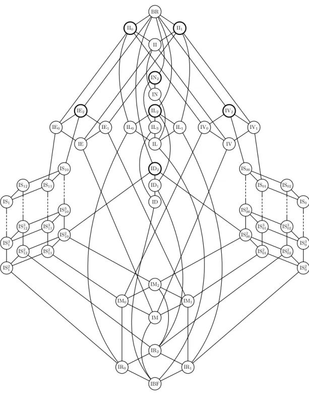
Just as a convenient shorthand let us denote the co-clone that is invariant underB by IB, hence IB = Inv(B). Hence, for example, IE2 is the co-clone of Horn relations and IL2 is the co-clone of affine relations. The co-clone of all relations is denoted by BR. The complete structure of the lattice of co-clones is given by Fig. 2. A look at this graph shows that below the class BR there exist seven maximal closed classes of Boolean relations (circled bold in Fig. 2). Hence if we want to know whether all Boolean relations can be “simulated” by conjunctive queries built with constraints from a given setS, then we have to check thatS is not included in one of these seven classes. This is the same idea as in part 1 of this column where we used the five Post classes to obtain a completeness criterion for classes of Boolean functions and used it to prove that the nand-function is a base of BF.
Example 1.9. Let be S = {Ror3,0, Ror3,1, Ror3,2, Ror3,3}. Clearly Ror3,0 is not 0-valid and Ror3,3 is not 1-valid. Using our tests we can show that Ror3,0 is not Horn, because (1,0,0)∈Ror3,0 and (0,0,1) ∈ Ror3,0 but (0,0,0) 6∈ Ror3,0. Similarly we have that Ror3,3 is not anti-Horn, because (1,0,0) ∈ Ror3,3 and (0,1,1) ∈ Ror3,3 but (1,1,1)6∈ Ror3,3. Additionally Ror3,0 is not bijunctive, because (1,0,0) ∈ Ror3,0, (0,1,0) ∈ Ror3,0 and (0,0,1) ∈ Ror3,0 but (0,0,0) 6∈ Ror3,0. Next note that (1,0,0) ∈ Ror3,3, (0,1,0) ∈ Ror3,3 and (0,0,1) ∈ Ror3,3 but (1,1,1) 6∈ Ror3,3, which shows that Ror3,3 is not affine. Finally we have that (0,0,0)6∈Ror3,0 but (1,1,1)∈ Ror3,0 showing that Ror3,0 is not complementive. Hence we have that the co-clone of S is II2 = BR, which gives that COQ(S) is the set of all Boolean relations. In fact, our argument above shows that already COQ({Ror3,0, Ror3,3}) = BR, the set of all relations.
2 The Complexity of Constraint Satisfaction Problems
The main topic in this section is the complexity of the satisfiability problem for S-formulas, de- noted by SAT(S). Comparing conjunctive queries withS-formulas, the only difference is that in the former some of the variables are existentially quantified, but certainly this does not lead to a differ- ent complexity of the satisfiability problem. Formally, if SAT(COQ(S)) denotes the satisfiability problem for conjunctive queries over S, then:
Proposition 2.1. SAT(S) is polynomial-time equivalent toSAT(COQ(S)).
Thus it is clear that the algebraic correspondence described above can be of use to deter- mine the complexity of constraint satisfaction problems. For instance, let us consider the relation ROne-Exactly. We have seen above thath{ROne-Exactly}iis the set of all Boolean relations, hence so is
IR0 IR1
IBF IR2 IM
IM0 IM1
IM2
IS21 IS31 IS1
IS212 IS312 IS12
IS211 IS311 IS11
IS210 IS310 IS10
IS20 IS30 IS0
IS202 IS302 IS02
IS201 IS301 IS01
IS200 IS300 IS00 ID2
ID ID1 IL2
IL
IL0 IL3 IL1 IE2
IE
IE0 IE1
IV2
IV IV1 IV0
II0 II1
IN2 II BR
IN
Figure 2: Graph of all co-clones
COQ({ROne-Exactly,Eq}) by Proposition 1.7. Therefore, the satisfiability problem SAT({ROne-Exactly,Eq}) is as hard as the general propositional satisfiability problem, i.e., it is NP-complete.
As a consequence we have that the complexity of SAT(S∪{Eq}) is characterized by the co-clone generated by S, hSi, or equivalently by its clone of polymorphisms Pol(S). We observe next that the equality relation actually is of no importance in the context of satisfiability; the reason is simply that in a CNF(S∪ {Eq}) we can delete a constraint Eq(x, y) and identify the variablesx, y in the rest of the formula [Jea98]. Thus we obtain:
Proposition 2.2. LetSbe a non-empty set of Boolean relations, thenSAT(S∪{Eq})is polynomial- time reducible toSAT(S). Hence,SAT(S) is polynomial-time equivalent to SAT(hSi).
The following two easy reductions provide the central tools to obtain a complexity classification of the satisfiability problem. The first one is obtained, if all constraints in one formula can be expressed by conjunctive queries over another constraint set:
Proposition 2.3. Let S1 and S2 be finite non-empty sets of Boolean relations. If COQ(S1) ⊆ COQ(S2), then SAT(S1) is polynomial-time reducible toSAT(S2).
Proof. If COQ(S1) ⊆ COQ(S2), then in particular every relation in S1 can be expressed by a conjunctive query over S2. Thus, given an S1-formula, one can construct an S2-formula in locally replacing (in each conjunct) every relation fromS1by its equivalent conjunctive query in COQ(S2) and simply deleting the existential quantifiers. This local replacement clearly provides a polynomial- time (and even logarithmic-space) reduction from SAT(S1) to SAT(S2).
Combining this with Proposition 1.7 and Theorem 1.5 we obtain the following reduction:
Theorem 2.4 [Jea98]. Let S1 and S2 be finite non-empty sets of Boolean relations. IfPol(S2)⊆ Pol(S1), then SAT(S1) is polynomial-time reducible toSAT(S2).
Proof. By Theorem 1.8, if Pol(S2) ⊆Pol(S1), then Inv(Pol(S1))⊆Inv(Pol(S2)). Hence, following Theorem 1.5,hS1i ⊆ hS2i. Thus, according to Proposition 1.7, COQ(S1∪ {Eq})⊆COQ(S2∪ {Eq}) and hence COQ(S1) ⊆ COQ(S2 ∪ {Eq}). Therefore, according to Proposition 2.3, SAT(S1) is polynomial-time reducible to SAT(S2∪ {Eq}), and thus to SAT(S2) by Proposition 2.2.
We are now in a position to prove Schaefer’s main result, a dichotomy theorem for satisfiability of constraint satisfaction problems which can be stated as follows:
Theorem 2.5 [Sch78]. Let S be a set of Boolean relations. If S is 0-valid or 1-valid or Schaefer thenSAT(S) is polynomial-time decidable, in all other casesSAT(S) is NP-complete.
We now give a proof of Theorem 2.5 making use of the algebraic correspondence described above and of the lattice of co-clones. Our presentation follows an argument sent to the authors in an e-mail correspondence by Phokion Kolaitis, but is implicit in the papers by Jeavons and his group (see, e.g., [JCG97, JCG99]) and in Dalmau’s Ph. D. thesis [Dal00].
LetS be a set of constraints. We make a case distinction, making use of the graph of co-clones in Fig. 2.
1. S⊆II0, i.e., Pol(S)⊇I0. Then we see thatS must contain the all-zero vector, i.e., S is 0-valid.
Hence every instance of CSP(S) is satisfiable via the all-0 vector.
2. S ⊆ II1, i.e., Pol(S) ⊇ I1. In this case, S must be 1-valid, and every instance of CSP(S) is satisfiable via the all-1 vector.
The maximal co-clones not included in II1 or II0 are BR, IN2, IE2, IL2, IV2, and ID2. We consider these in turn.
3. S⊆IE2, i.e., Pol(S)⊇E2and contains the functionx∧y. This means that every relationR ∈S is closed under coordinate-wise∧, henceR is Horn. Satisfiability for Horn formulas is known to be polynomial-time solvable by the so called “Horn algorithm” (HORNSAT∈P, [Pap94, p. 78-79]).
4. S ⊆IV2, i.e., Pol(S)⊇V2 and contains the function x∨y. Analogous to the above, we obtain that R can be represented by an anti-Horn-formula. Again, satisfiability is in P by a variation of the Horn algorithm.
5. S ⊆ IL2, i.e., Pol(S) ⊇ L2 and contains in particular its basis, the function x⊕y⊕z. This means that every constraint in R must be affine. A CSP with affine constraints can be looked at as an equation system over GF[2], hence satisfiability can be tested in polynomial time with the Gaussian elimination algorithm.
6. S⊆ID2, i.e., Pol(S)⊇D2 and contains in particular its basis, the functionxz∧yz∧xy, i.e., the majority function of arity 3. This means that every constraint inRmust be bijunctive. Satisfiability for 2-CNF formulas is polynomial-time solvable (2SAT is even in NL, [Pap94, p. 184-185]).
The remaining cases are now those of the classes BR = II2 and IN2. We will prove that if hSi = IN2, then SAT(S) is NP-complete. According to Theorem 2.4 this will be sufficient since II2⊇IN2, thus concluding the proof.
7. hSi = IN2, i.e., Pol(S) = N2. In this case, hSi is the set of all Boolean relations R that are closed under all projection functions and their negations. In particular, hSi contains the ternary relation RNAE defined in Example 1.1. (It can be shown that in fact, hSi is equal to the set of all complementive relations.) Looking at CNF formulas with clauses that are applications of the constraint RNAE, we see that we deal with a particular satisfiability problem for 3-CNF formulas where we ask if there is an assignment that in every clause makes one variable false and one variable true (stated otherwise: not all three variables in a clause receive the same truth assignment). This is the so called NOT-ALL-EQUAL-3SAT problem which is known to be NP-complete, see, e.g., [Pap94]. Hence, also in this case, SAT(S) is NP-complete, and the proof of Schaefer’s dichotomy theorem is finished.
The only cases for Pol(S) that lead to an NP-complete satisfiability problem are those of I2 and N2. A common property of these classes is the following: Say that ann-ary functionf isessentially unary if it is not constant and depends on only one of its arguments, i.e., there is some i, 1≤i≤n and some unary non-constant Boolean function f0 such that f(x1, . . . , xi, . . . , xn) = f0(xi). Of course, the only possibilities for f0 are the unary identity or the unary negation. Thus we obtain the following corollary:
Corollary 2.6 [JC95, JCG99]. Let S be a set of Boolean constraints. If Pol(S) consists of only essentially unary functions, then SAT(S) is NP-complete, otherwise SAT(S) is polynomial-time solvable.
Further Complexity Results
In the context of Boolean constraint satisfaction, not only the satisfiability problem was looked at, but many more problems were classified w.r.t. their computational complexity. Considering different
versions of satisfiability, equivalence, optimization and counting problems, dichotomy theorems for classes as NP, US, MaxSNP, OptP, and #P were obtained [Cre95, CH96, CH97, KS98, Jub99, BHRV02, RV03, KK03, BHRV04], see also the monograph [CKS01]. Satisfiability and learnability of generalized quantified Boolean formulas were studied by Dalmau [Dal00]. Also, the study of Schaefer’s formulas lead to remarkable results about approximability of optimization problems in the constraint satisfaction context [KST97, KSW97, Zwi98].
Connections between algebraic theory and the computational complexity of constraint satisfac- tion problems were originally developed for studying decision problems where the question is to decide the existence of a solution. Until now, only Schaefer’s original dichotomy theorem for sat- isfiability and the metaproblem in the upcoming section have been re-proven making use of Post’s lattice. Only in a very recent paper, Krokhin and Jonsson [KJ03] have shown that this approach can lead to general results for a wider range of problems with different computational properties.
They have studied the complexity of recognizing frozen variables (i.e., variables that take the same values in all possible solutions) in an S-formula and completely classified the complexity of this problem. We consider it interesting to give an alternative proof along the same lines of, e.g., the dichotomy theorem for counting the number of satisfying assignments from [CH96].
3 The Metaproblem: The Complexity of the Co-clones
We have given a definition of co-clones as objects that are useful for the complexity study of problems for Boolean constraints. But how complicated are the co-clones themselves, i.e., how difficult is it to decide whether a relation given in a reasonably compact form, e.g. a propositional formula over{and,or,not}, is element of a specified co-clone?
Definition 3.1. For a co-clone S, we define
coMEM(S) ={F |F is propositional formula and the relation represented byF is inS}.
Analogously to duality for Boolean functions (in part I of this column), we define the notion of duality for Boolean relations.
Definition 3.2. LetRbe ann-ary Boolean relation. Thedual relationofRis defined by dual(R) = (a1, . . . , an)
(a1, . . . , an)∈R . For a set of Boolean relations S let dual(S) =
dual(R) R ∈ S . Note that the dual-operator establishes a bijection between the elements ofS and the elements of dual(S).
We get the following easy connection between duality of Boolean functions and Boolean rela- tions:
Proposition 3.3. Let f be a Boolean function and R be a Boolean relation. Then f preservesR if and only if dual(f) preserves dual(R).
The following result about the complexity of the co-clones appeared in [Cre98]. We now present a proof relying on the Galois correspondence between Boolean constraints and function.
Theorem 3.4. If S is the co-clone of all Boolean relations, the co-clone of all 0-valid relations, the co-clone of all1-valid relations, or the co-clone of all relations that are both0- and1-valid (i.e., S ∈ {II2,II0,II1,II}), then the problem coMEM(S) is inP. For every other co-cloneS, the problem coMEM(S) is coNP-complete.
Proof. As before, we will not distinguish between formulas and the relations they represent and we will speak, e.g., of tuples in a relationR as well as tuples in a formula F.
The claim is obvious for the easy cases, since to check if a relation R is 0-valid or 1-valid one just has to check if one tuple is inR.
For a Boolean function f:{0,1}m → {0,1} and tuples α1, . . . , αm ∈ {0,1}n, letf(α1, . . . , αm) be then-tuple obtained by coordinate-wise applyingf to theαi’s.
First of all, observe, that coMEM(S) is in coNP for all co-clonesS: For a given n-ary propo- sitional formula F, guess any function f from a fixed basis of Pol(S). Suppose, that f is m-ary.
Guess m tuples α1, . . . , αm ∈ {0,1}n. Test, whether these tuples are inF. If this is not the case, accept. If they are all in F, then accept if and only if f(α1, . . . , αm) ∈ F. Then the relation represented by F is in S if and only if all guesses are successful.
Let TAUT be the set of tautological propositional formulas, which is known to be coNP- complete. We will reduce TAUT to coMEM(S) for all co-clones S that do not belong to the easy cases. Take a n-ary propositional formula H, let g(H)(x1, . . . , xn) =def H(x1, . . . , xn) ∧ H(x1, . . . , xn) and let
h(H) = (x1 =x2)∧(g(H)(y1, . . . , yn)∨z1)∧(H(u1, . . . , un)∨z2∨z3∨z4).
If H ∈TAUT, then h(H) ≡x1 =x2 and therefore h(H) ∈S. On the other hand, if H /∈TAUT, there is anα∈ {0,1}nsuch that H(α) = 0.
– Observe that h(H)(0,0, α,0, α,1,0,0) = 1 6= h(H)(1,1, α,1, α,0,1,1). Thus h(H) is not complementive.
– Observe that the tuples (0,0, α,0, α,1,0,0) and (0,0, α,0, α,0,1,0) are in h(H), but on the other hand,and((0,0, α,0, α,1,0,0),(0,0, α,0, α,0,1,0)) = (0,0, α,0, α,0,0,0) is not inh(H).
Thush(H) is not closed underand and therefore it is not equivalent to a Horn-formula.
– Let f(x, y, z) = xy ∨xz ∨yz, i.e., f is a basis for clone D2. Observe that the tuples (0,0, α,0, α,1,0,0), (0,0, α,0, α,0,1,0), (0,0, α,0, α,0,0,1) are in h(H), but on the other hand,f((0,0, α,0, α,1,0,0),(0,0, α,0, α,0,1,0),(0,0, α,0, α,0,0,1))) = (0,0, α,0, α,0,0,0) is not inh(H). Thush(H) is not bijunctive.
– Letf(x, y, z) =x⊕y⊕z, i.e.,f is a basis for clone L2. Observe that the tuples (0,0, α,0, α,1,1,0),
(0,0, α,0, α,0,1,0), (0,0, α,0, α,1,0,0) are inh(H), but on the other hand,f((0,0, α,0, α,1,1,0),(0,0, α,0, α,0,1,0),(0,0, α,0, α,1,0,0))
= (0,0, α,0, α,0,0,0) is not in h(H). Thush(H) is not affine.
Thus, membership for co-clones that are complementive, Horn, bijunctive, or affine is coNP- complete. Finally, Proposition 3.3 yields coNP-completeness for co-clones that are anti-Horn.
References
[Art98] E. Artin. Galois Theory. Dover Publications, 1998.
[BHRV02] E. B¨ohler, E. Hemaspaandra, S. Reith, and H. Vollmer. Equivalence and isomorphism for Boolean constraint satisfaction. In Computer Science Logic, volume 2471 of Lecture Notes in Computer Science, pages 412–426, Berlin Heidelberg, 2002. Springer Verlag.
[BHRV04] E. B¨ohler, E. Hemaspaandra, S. Reith, and H. Vollmer. The complexity of Boolean constraint iso- morphism. InProceedings 21st Symposium on Theoretical Aspects of Computer Science, Lecture Notes in Computer Science, Berlin Heidelberg, 2004. Springer Verlag. To appear.
[BKKR69] V. G. Bodnarchuk, L. A. Kaluˇznin, V. N. Kotov, and B. A. Romov. Galois theory for Post algebras. i, ii. Cybernetics, 5:243–252, 531–539, 1969.
[CH96] N. Creignou and M. Hermann. Complexity of generalized satisfiability counting problems. In- formation and Computation, 125:1–12, 1996.
[CH97] N. Creignou and J.-J. H´ebrard. On generating all solutions of generalized satisfiability problems.
Informatique Th´eorique et Applications/Theoretical Informatics and Applications, 31(6):499–511, 1997.
[CKS01] N. Creignou, S. Khanna, and M. Sudan. Complexity Classifications of Boolean Constraint Sat- isfaction Problems. Monographs on Discrete Applied Mathematics. SIAM, 2001.
[Cre95] N. Creignou. A dichotomy theorem for maximum generalized satisfiability problems. Journal of Computer and System Sciences, 51:511–522, 1995.
[Cre98] N. Creignou. Complexity versus stability. Information Processing Letters, 68:161–165, 1998.
[Dal00] V. Dalmau. Computational complexity of problems over generalized formulas. PhD thesis, De- partment de Llenguatges i Sistemes Inform`atica, Universitat Polit´ecnica de Catalunya, 2000.
[DP92] R. Dechter and J. Pearl. Structure identification in relational data.Artificial Intelligence, 48:237–
270, 1992.
[Gei68] D. Geiger. Closed systems of functions and predicates. Pac. J. Math, 27(2):228–250, 1968.
[JC95] P. G. Jeavons and D. A. Cohen. An algebraic characterization of tractable constraints. InCom- puting and Combinatorics. First International Conference COCOON’95, volume 959 ofLecture Notes in Computer Science, pages 633–642, Berlin Heidelberg, 1995. Springer Verlag.
[JCG97] P. G. Jeavons, D. A. Cohen, and M. Gyssens. Closure properties of constraints. Journal of the ACM, 44(4):527–548, 1997.
[JCG99] P. G. Jeavons, D. A. Cohen, and M. Gyssens. How to determine the expressive power of con- straints. Constraints, 4:113–131, 1999.
[Jea98] P. G. Jeavons. On the algebraic structure of combinatorial problems. Theoretical Computer Science, 200:185–204, 1998.
[Jub99] L. Juban. Dichotomy theorem for generalized unique satisfiability problem. InProceedings 12th Fundamentals of Computation Theory, volume 1684 ofLecture Notes in Computer Science, pages 327–337. Springer Verlag, 1999.
[KJ03] A. Krokhin and P. Jonsson. Recognizing frozen variables in constraint satisfaction problems.
Technical Report TR03-062, ECCC Reports, 2003.
[KK03] L. M. Kirousis and P. Kolaitis. The complexity of minimal satisfiability problems. Information and Computation, 187(1):20–39, 2003.
[Kol03] P. Kolaitis. Constraint satisfaction, databases, and logic. InProceedings 18th International Joint Conference on Artificial Intelligence, pages 1587–1595, 2003.
[KS98] D. Kavvadias and M. Sideri. The inverse satisfiability problem. SIAM Journal of Computing, 28(1):152–163, 1998.
[KST97] S. Khanna, M. Sudan, and L. Trevisan. Constraint satisfaction: the approximability of mini- mization problems. In Proceedings 12th Computational Complexity Conference, pages 282–296.
IEEE Computer Society Press, 1997.
[KSW97] S. Khanna, M. Sudan, and D. Williamson. A complete classification of the approximability of maximization problems derived from Boolean constraint satisfaction. In Proceedings 29th Symposium on Theory of Computing, pages 11–20. ACM Press, 1997.
[KV00] P. Kolaitis and M. Vardi. Conjunctive-query containment and constraint satisfaction. Journal of Computer and System Sciences, 61:302–332, 2000.
[Pap94] C. H. Papadimitriou. Computational Complexity. Addison-Wesley, Reading, MA, 1994.
[Pip97] N. Pippenger. Theories of Computability. Cambridge University Press, Cambridge, 1997.
[PK79] R. P¨oschel and L. A. Kaluˇznin. Funktionen- und Relationenalgebren. Deutscher Verlag der Wissenschaften, Berlin, 1979.
[P¨os01] R. P¨oschel. Galois connection for operations and relations. Technical Report MATH-LA-8-2001, Technische Universit¨at Dresden, 2001.
[RV03] S. Reith and H. Vollmer. Optimal satisfiability for propositional calculi and constraint satisfaction problems. Information and Computation, 186(1):1–19, 2003.
[Sch78] T. J. Schaefer. The complexity of satisfiability problems. In Proccedings 10th Symposium on Theory of Computing, pages 216–226. ACM Press, 1978.
[Zwi98] U. Zwick. Finding almost-satisfying assignments. In Proceedings 30th Symposium on Theory of Computing, pages 551–560. ACM Press, 1998.
Correction: The statement of Theorem 2.3 of the first part of our column should read as follows:
“If B⊆V orB⊆L orB ⊆E then CVP(B)∈NC; in all other cases CVP(B) is P-complete.”