Picture of title page provided by M. Sebastian Pauletti.
Contents
1 Variational Formulation and Finite Element Method 3
1.1 Classical vs Adaptive Approximation . . . . 3
1.2 Sobolev Spaces . . . . 4
1.3 Variational Formulation . . . . 5
1.3.1 Model Problem . . . . 5
1.3.2 General 2
ndOrder Elliptic Operator . . . . 6
1.3.3 Neumann Problem . . . . 6
1.3.4 The H (div; Ω) System . . . . 7
1.3.5 The Stokes System . . . . 7
1.3.6 Dirichlet Boundary Condition via Lagrange Multiplier . . . . 7
1.4 The Inf-Sup Theory . . . . 8
1.5 The Galerkin Method . . . . 11
1.6 Error Analysis . . . . 11
1.7 The Finite Element Method . . . . 12
1.8 Polynomial Interpolation . . . . 13
1.9 Exercises of Lecture 1 . . . . 15
2 Bisection and Constructive Approximation 17 2.1 Newest Vertex Bisection . . . . 17
2.2 Properties of Bisection . . . . 19
2.3 Complexity of REFINE . . . . 22
2.4 Principle of Equidistribution . . . . 24
2.5 Construction of Optimal Meshes . . . . 25
2.6 Exercises of Lecture 2 . . . . 27
3 A Posteriori Error Analysis 29 3.1 Residual Structure . . . . 29
3.2 Ingredients . . . . 30
3.3 Derivation of the Upper Bound . . . . 31
3.4 Sharpness of the Upper Bound . . . . 32
3.5 Interior Residual . . . . 32
3.6 Jump Residual . . . . 33
3.7 Alternative Estimators . . . . 36
3.8 Exercises of Lecture 3 . . . . 37
4 Convergence of AFEM 39 4.1 Convergence of AFEM without Rate . . . . 39
4.2 Modules of AFEM for the Model Problem . . . . 40
4.3 Contraction Property of AFEM . . . . 42
4.4 Example: Discontinuous Coefficients . . . . 44
4.5 Exercises of Lecture 4 . . . . 45
5 Quasi-Optimal Cardinality of AFEM 47 5.1 Approximation Class . . . . 47
5.2 Cardinality of M
k. . . . 49
5.3 Quasi-Optimal Cardinality . . . . 51
5.4 Separate Marking . . . . 51
5.5 Exercises of Lecture 5 . . . . 53
6 AFEM for Geometric PDE and Applications 54 6.1 Finite Element Representation of Manifolds . . . . 54
6.2 Basic Differential Geometry . . . . 55
6.3 AFEM: Modules and Algorithm . . . . 58
6.4 Conditional Contraction Property of AFEM . . . . 60
Lecture 1 Variational Formulation and Finite Element Method
This lecture starts with a comparison in 1D between uniform and suitably graded meshes which sets the tone for adaptivity. It follows with a brief review of Sobolev spaces along with the classical and variational formulation of several elliptic partial differential equations (PDE) that play a relevant role in the subsequent analysis. The lecture concludes with a complete discussion of the inf-sup theory and applications.
1.1 Classical vs Adaptive Approximation
We present a simple 1D example, due to DeVore [29], that compares the approximation properties of uniform and graded meshes. Given Ω = (0, 1), a partition T
N= { x
i}
Ni=0of Ω
0 ≤ x
0< x
1< · · · < x
n< · · · < x
N= 1
and a continuous function u : Ω → R , we consider the problem of interpolating u by a piecewise constant function U
Nover T
N. We measure the error in the max-norm.
Case 1: W
∞1-Regularity. Let u ∈ W
∞1(Ω) and
U
N(x) = u(x
n−1) for all x
n−1≤ x < x
n. Since
| u(x) − U
N(x) | = | u(x) − u(x
n−1) | =
Z
x xn−1u
′(s) ds
≤ h
nk u
′k
L∞(Ω), we conclude
k u − U
Nk
L∞(Ω)≤ 1
N k u
′k
L∞(Ω)(1.1)
for a quasi-uniform partition T
Nwith meshsize h
n= 1/N of the domain of u. Note that the same integrability is used on both sides of (1.1).
Case 2: W
11-Regularity. We want to obtain the same decay N
−1but with weaker regularity of u.
Consider the (non-decreasing) function
φ(x) = Z
x0
| u
′(s) | ds
which satisfies φ(0) = 0, φ(1) = 1 provided k u
′k
L1(Ω)= 1. Let T
Nsatisfy Z
xnxn−1
| u
′(s) | ds = φ(x
n) − φ(x
n−1) = 1 N ,
which corresponds to a uniform partition of the range of φ rather than the domain of u. Then, for x ∈ [x
n−1, x
n],
| u(x) − u(x
n−1) | ≤ Z
xxn−1
| u
′(s) | ds ≤ Z
xnxn−1
| u
′(s) | ds = 1 N whence
k u − U
Nk
L∞(Ω)≤ 1
N k u
′k
L1(Ω). (1.2)
We see that Case 2 exhibits the same asymptotic decay as Case 1 in the maximum norm. The following comments are in order for Case 2.
Remark 1.1 (Equidistribution). The optimal mesh T
Nequidistributes the max-error. This mesh is graded
instead of uniform, but it may not be adequate for another function u.
Remark 1.2 (Integrability). The regularity of u is measured in W
11(Ω) instead of W
∞1(Ω). This exchange of integrability, between left and right-hand side of (1.2), is at the heart of the matter and the very reason why suitably graded meshes achieve optimal asymptotic error decay for singular functions. By those we mean functions which are not in the usual linear Sobolev scale, say W
∞1(Ω) in this example, but rather in a nonlinear scale. We will get back to this issue in Lectures 2 and 5.
1.2 Sobolev Spaces
Since approximability and regularity of functions are intimately related concepts, it is convenient to briefly review definitions, basic concepts and properties of L
p-based Sobolev spaces with emphasis on 1 ≤ p ≤ ∞ and dimension d ≥ 1.
Definition 1.1 (Sobolev space). Given k ∈ N and 1 ≤ p ≤ ∞ , we define W
pk(Ω) := { v : Ω → R | D
αv ∈ L
p(Ω) for all | α | ≤ k }
where D
αv = ∂
xα11· · · ∂
xαddv stands for the weak derivative of order α. The corresponding norm and seminorm for 1 ≤ p < ∞ are
k v k
Wpk(Ω):= X
|α|≤k
k D
αv k
pLp(Ω) 1/p| v |
Wpk(Ω):= X
|α|=k
k D
αv k
pLp(Ω) 1/p,
with obvious changes for p = ∞ .
Definition 1.2 (Sobolev number). The Sobolev number of W
pk(Ω) is defined by
sob(W
pk) := k − d/p. (1.3)
This definition is motivated by the scaling of the seminorm in W
pk(Ω). Consider the change of variables b
x =
h1x for all x ∈ Ω, which transforms the domain Ω into Ω and functions defined over Ω into functions b b v defined over Ω. Then b
|b v |
Wpk(bΩ)= h
k−d/p| v |
Wpk(Ω).
Properties of Sobolev Spaces W
pk(Ω). We summarize now, but not prove, several important properties of Sobolev spaces which play a key role later. We refer to [32, 34, 36] for details.
• Embedding: Let m > k, sob(W
pm) > sob(W
qk), with ∂Ω Lipschitz. Then W
pm(Ω) ֒ → W
qk(Ω) (compact).
Note that v(x) = log log
|x|2∈ W
d1(Ω) \ L
∞(Ω) where Ω is the unit ball of R
d, and sob(W
d1) = 1 − d/d = 0 = 0 − d/ ∞ = sob(L
∞).
Therefore, equality between Sobolev numbers cannot be expected in the embedding theorem.
• Density: If ∂Ω is Lipschitz, then C
∞(Ω) is dense in W
pk(Ω).
• Poincar´ e Inequality I: The following inequality holds
v − | Ω |
−1Z
Ω
v
L2(Ω). diam(Ω) k∇ v k
L2(Ω)for all v ∈ W
21(Ω). (1.4)
The spaces H
k(Ω). We let H
k(Ω) = W
2k(Ω) for k ≥ 1 and, in particular, H
1(Ω) = W
21(Ω).
These are Hilbert spaces with scalar product h u, v i = P
|α|≤k
m R
Ω
D
αuD
αv for all u, v ∈ H
k(Ω). Let H
01(Ω) be the completion of C
0∞(Ω) within H
1(Ω). If Ω is bounded, then H
01(Ω) is a strict subspace H
1(Ω) because 1 ∈ H
1(Ω) \ H
01(Ω) and the following properties are valid.
• Poincar´ e Inequality II: The following inequality holds
k v k
L2(Ω). diam(Ω) k∇ v k
L2(Ω)for all v ∈ H
01(Ω). (1.5)
• Norm equivalence: The norm and seminorm in H
01(Ω) are equivalent, namely, there exists a constant c(Ω) depending on Ω only so that
| v |
1,Ω≤ k v k
1,Ω≤ c(Ω) | v |
1,Ωfor all ∈ H
01(Ω). (1.6)
The space H
−1(Ω). This is the dual of H
01(Ω), i.e. the space of all continuous and linear functionals from H
01(Ω) to R equipped with the operator norm
k f k
H−1(Ω)= sup
v∈H01(Ω)
h f, v i
| v |
1,Ω= sup
|v|1,Ω=1
h f, v i .
The spaces H
1/2(∂Ω) and H
−1/2(∂Ω). If v ∈ C
1( ¯ Ω), then the following inequality can be derived by localization and flattening of the boundary:
k v k
L2(∂Ω)≤ c(Ω) k v k
H1(Ω),
where c(Ω) depends on Ω only; the proof is elementary if ∂Ω is flat. By a density argument this inequality is valid for all v ∈ H
1(Ω). Therefore, functions in H
1(Ω) admit traces or restrictions to the boundary and the resulting functions are in L
2(∂Ω). The space of traces of functions in H
1(Ω) is denoted by H
1/2(∂Ω) and turns out to be strictly smaller than L
2(∂Ω). The dual of H
1/2(∂Ω) is called H
−1/2(∂Ω).
1.3 Variational Formulation
We consider 2
ndorder elliptic PDE in divergence form. Multiplication by a test function v and integration by parts leads to the abstract problem (weak or variational formulation)
u ∈ V : B [u, v] = h f, v i for all v ∈ V (1.7)
where V is Hilbert space, f ∈ V
∗the dual of V , and B is a bilinear form with properties to be specified below. We now consider several examples that are relevant for the rest of this review.
1.3.1 Model Problem
Let A(x) ∈ R
d×dbe (uniformly) symmetric positive definite (SPD) over Ω, i.e.
α
1| ξ |
2≤ ξ
TA(x)ξ ≤ α
2| ξ |
2for all x ∈ Ω, ξ ∈ R
dwith 0 < α
1≤ α
2independent of x ∈ Ω. The variational formulation of
− div(A(x) ∇ u) = f in Ω
u = 0 on ∂Ω (1.8)
is as follows: given V = H
01(Ω), V
∗= H
−1(Ω), and f ∈ V
∗, let u ∈ V : B [u, v] =
Z
Ω
∇ v · A(x) ∇ u = h f, v i for all v ∈ V . (1.9) This problem is equivalent to a minimization in V of the quadratic functional
J [v] = 1
2 B [v, v] − h f, v i .
We introduce the energy norm ||| v |||
2Ω= B [v, v], which plays a relevant role in Lectures 4 and 5.
1.3.2 General 2
ndOrder Elliptic Operator
Let A be (uniiformly) SPD as in § 1.3.1, and b ∈ [L
∞(Ω)]
dand c ∈ L
∞(Ω). Consider
− div(A(x) ∇ u) + b(x) · ∇ u + c(x)u = f in Ω u = 0 on ∂Ω The variational formulation reads: given V = H
01(Ω), V
∗= H
−1(Ω), and f ∈ V
∗, let
u ∈ V : B [u, v] = Z
Ω
∇ u · A(x) ∇ v + b ∇ uv + c uv = h f, v i for all v ∈ V .
If b 6 = 0 this problem cannot be written as a minimization of a suitable quadratic functional J . However, if b = 0 and c ≥ 0, then B induces a scalar product, energy norm, and quadratic functional J as in § 1.3.1.
1.3.3 Neumann Problem
Let A be (uniformly) SPD as in § 1.3.1. If ν is the unit outer normal to ∂Ω, then the problem
− div(A(x) ∇ u) = h in Ω ν · A(x) ∇ u = g on ∂Ω
has the following variational formulation: given V = H
1(Ω), V
∗= (H
1(Ω))
∗, and h ∈ L
2(Ω), g ∈ L
2(∂Ω), let u ∈ V : B [u, v] =
Z
Ω
∇ v · A(x) ∇ u = Z
Ω
hv + Z
∂Ω
gv = h f, v i for all v ∈ V .
This problem is equivalent to the minimization in V of the quadratic functional J [v] =
12B [v, v] − h f, v i . It is clear upon taking v = 1 ∈ V that the following compatibility condition between data h and g is necessary for existence of a solution u ∈ V : Z
Ω
h + Z
∂Ω
g = 0.
In addition, we observe that the functional f reduces to h if restricted to H
01(Ω). We conclude that V
∗is
different from H
−1(Ω).
1.3.4 The H(div; Ω) System
Given a vector field f , let the vector field u be the classical solution of u − ∇ div u = f in Ω
u · ν = 0 on ∂Ω.
Let V = H (div; Ω) be the space of vector fields v ∈ [L
2(Ω)]
dsuch that div v ∈ L
2(Ω). The variational formulation of the problem above reads: given f ∈ V
∗, let
u ∈ V : B [u, v] = Z
Ω
u · v + div u div v = h f , v i for all v ∈ V .
This is equivalent to the minimization in V of the quadratic functional J[v] =
12B [v, v] − h f , v i . 1.3.5 The Stokes System
Given a vector field f , let (u, p) be the velocity-pressure pair which satisfies the momemtum and incom- pressibility equations and no-slip boundary condition:
− ∆u + ∇ p = f in Ω div u = 0 in Ω
u = 0 on ∂Ω.
Consider the Hilbert space product V = [H
01(Ω)]
d× L
20(Ω), where L
20(Ω) is the space of square integrable functions with zero meanvalue. The variational formulation reads:
(u, p) ∈ V : B [(u, p), (v, q)] = Z
Ω
∇ u : ∇ v − p div u + q div u = h f , v i for all (v, q) ∈ V . This problem can be viewed as a saddle point problem, in which the pressure p is the Lagrange multiplier for the divergence-free constraint div u = 0 [13, 15, 16, 17, 35].
1.3.6 Dirichlet Boundary Condition via Lagrange Multiplier
Given f ∈ H
−1(Ω) and g ∈ H
1/2(∂Ω), consider the following Dirichlet problem [3]:
− ∆u + u = f in Ω u = g on ∂Ω.
We can view the boundary condition as a constraint, and thereby enforce it via a Lagrange multiplier λ. In fact, if we multiply the PDE by a test function v ∈ H
1(Ω) and integrate by parts, then we arrive at the following variational formulation: given V = H
1(Ω) × H
−1/2(∂Ω), let
(u, λ) ∈ V : B [(u, λ), (v, µ)] = Z
Ω
∇ u · ∇ v + uv − Z
∂Ω
λv − µu = h f, v i
Ω+ h g, v i
∂Ωfor all (v, µ) ∈ V ;
note that the multiplier satisfies λ = ∂
νu formally. This is also a saddle point problem [13, 15, 16, 17, 35].
1.4 The Inf-Sup Theory
We now present a functional analytic theory, the so-called inf-sup theory, that yields existence, uniqueness and well poseness of the variational problems introduced above. We first recall two fundamental results from functional analysis which lead to Theorem 1.5 below, a generalization of the Lax-Milgram theorem.
Theorem 1.3 (Projection Theorem). Let V be a Hilbert space and Z be a non-empty and closed subspace.
Then there exists a linear mapping P : V → Z such that k v − P v k
V= dist(v, Z ) = inf
z∈Z
k v − z k
Zfor all v ∈ V . An equivalent characterization of P is given by
h v − P v, z i
V= 0 for all z ∈ Z .
Let V , W be a pair of Hilbert spaces with scalar products h· , ·i
V, h· , ·i
Wand associated norms k · k
V, k · k
W. We denote by L( V ; W ) the space of linear and continuous operators from V into W , and L( V ) = L( V ; V ).
Theorem 1.4 (Riesz Representation Theorem). If V is a Hilbert space and V
∗is its dual, then the map J : V → V
∗defined by
h Jv, w i
V∗×V:= h v, w i
Vfor all v, w ∈ V is an isometric isomorphism J ∈ L( V , V
∗), i. e.,
k Jv k
V∗= k v k
Vfor all v ∈ V . Let B : V × W → R be a continuous bilinear form with operator norm
β = kBk = sup
v∈V
sup
w∈W
B [v, w]
k v k
Vk w k
W. (1.10)
Theorem 1.5 (Banach-Neˇcas). There exists a unique linear operator B ∈ L( V , W ) such that h Bv, w i
W= B [v, w] for all v ∈ V , w ∈ W
with operator norm
k B k = β.
Moreover, the bilinear form B satisfies
there exists α > 0 such that α k v k
V≤ sup
w∈W
B [v, w]
k w k
Wfor all v ∈ V , (1.11) for every 0 6 = w ∈ W there exists v ∈ V such that B [v, w] 6 = 0, (1.12) if and only if B : V → W is an isomorphism with
k B
−1k
L(W,V)≤ α
−1. (1.13)
Proof. We proceed in several steps.
1
Existence of B. For fixed v ∈ V , the mapping B [v, · ] belongs to W
∗by linearity of B in the second component and continuity of B . Applying the Riesz Representation Theorem 1.4, we deduce the existence of Bv ∈ W such that
h Bv, w i
W= B [v, w] ∀ w ∈ W .
Linearity of B in the first argument and continuity of B imply B ∈ L( V ; W ). In view of (1.10), we get k B k
L(V;W)= sup
v∈V
k Bv k
Wk v k
V= sup
v∈V
sup
w∈W
h Bv, w i
k v k
Vk w k
W= sup
v∈V
sup
w∈W
B [v, w]
k v k
Vk w k
W= β.
2
Closed Range of B. The inf-sup condition (1.11) implies α k v k
V≤ sup
w∈W
h Bv, w i
k w k
W= k Bv k
Wfor all v ∈ V , (1.14) whence B is injective. To prove that the range B( V ) of B is closed in W , we let w
k= Bv
kbe a sequence such that w
k→ w ∈ W as k → ∞ . We need to show that w ∈ B( V ). Invoking (1.14), we have
α k v
k− v
jk
V≤ k B(v
k− v
j) k
W= k w
k− w
jk
W→ 0
as k, j → ∞ . Thus { v
k}
∞k=0is a Cauchy sequence in V and so it converges v
k→ v ∈ V as k → ∞ . Continuity of B yields
Bv = lim
k→∞
Bv
k= w ∈ B( V ), which shows that B( V ) is closed.
3
Surjectivity of B. We argue by contradiciton, i.e. assume B( V ) 6 = W . Invoking the Projection Theorem 1.3, we deduce the existence of 0 6 = w
0∈ B ( V )
⊥. This is equivalent to
w
06 = 0 and h w, w
0i = 0 for all w ∈ B( V ), or
w
06 = 0 and 0 = h Bv, w
0i = B [v, w
0] for all v ∈ V .
This in turn contradicts (1.12) and shows that B( V ) = W . Therefore, we conclude that B is an isomorphism from V onto W .
4
Property (1.13). We rewrite (1.14) as follows:
α k B
−1w k
V≤ k w k
Wfor all w ∈ W , which is (1.13) in disguise.
5
Property (1.13) implies (1.11) and (1.12). Compute inf
v∈V
sup
w∈W
B [v, w]
k v k
Vk w k
W= inf
v∈V
sup
w∈W
h Bv, w i k v k
Vk w k
W= inf
v∈V
k Bv k
Wk v k
V= inf
w∈W
k w k
Wk B
−1w k
V= 1 sup
w∈WkB−1wkV kwkW
= 1
k B
−1k ≥ α
which shows (1.11). Property (1.12) is a consequence of B being an isomorphism: there exists 0 6 = v ∈ V such that Bv = w and
B [v, w] = h Bv, w i = k w k
2W6 = 0.
This concludes the Theorem.
We now consider an abstract problem a bit more general than (1.7): given two Hilbert spaces V , W and f ∈ W
∗, an element in the dual space W
∗of W , find
u ∈ V : B [u, w] = h f, w i for all w ∈ W . (1.15)
To establish existence and uniqueness of (1.15), we need the following fundamental theorem due to Neˇcas
[47, Theorem 3.3] and Babuˇska [6, 7].
Theorem 1.6 (Existence and Uniqueness). The abstract problem (1.15) admits a unique solution u ∈ V for all f ∈ W
∗, which depends continuously on f if and only if the inf-sup conditions (1.11)-(1.12) are valid. In addition, the solution u of (1.15) satisfies the stability estimate
k u k
V≤ α
−1k f k
W∗for all f ∈ W
∗.
Proof. using the Riesz operator J
Wof Lemma 1.4, we can write (1.15) as follows:
h Bu, w i = h J
W−1f, w i for all w ∈ W ⇔ Bu = J
W−1f ∈ W .
Let (1.11)-(1.12) be valid. Then B is an isomorphism, which implies that there is a unique u ∈ V , and k u k
V= k B
−1J
Wf k
W≤ k B
−1kk f k
W∗≤ 1
α k f k
W∗.
Conversely, if (1.15) admits a unique solution for all f ∈ W
∗we deduce that B is an isomorphism, and the continuous dependence implies (1.13). Finally, Banach-Neˇcas Theorem 1.5 yields (1.11)-(1.12).
We stress that conditions (1.11)-(1.12) are necessary and sufficient for existence with continuous dependence on data. An important class of bilinear forms satisfying (1.11)-(1.12) is the following: we let V = W and say that B is coercive if
B [v, v] ≥ α k v k
2V∀ v ∈ V . (1.16)
Corollary 1.7 (Lax-Milgram Theorem). If V = W and B is coercive, then B : V → V
∗is an isomorphism and (1.15) admits a unique solution that satisfies (1.13).
Proof. Since (1.16) implies sup
w∈VB [v, w] ≥ B [v, v] ≥ α k v k
2Vfor all 0 6 = v ∈ V , both (1.11) and (1.12) follow immediately, whence Theorem 1.6 implies the assertion.
Examples. We now review the examples introduced above in light of this inf-sup theory.
• Coercivity (Lax-Milgram). Let V = W = H
01(Ω) and B be the bilinear form in either § 1.3.1 or § 1.3.2 with c − 1/2 div b ≥ 0. Then B is coercive with constant α = α
1. The same happens for the H(div; Ω) system, but in this case α = 1.
Consider now the Neumann problem of § 1.3.3. We have V = H
1(Ω) and B [1, 1] = 0, whence B is not coercive. However, if we restrict the space V = { v ∈ H
1(Ω) | R
Ω
v = 0 } , then Poincar´e inequality I implies coercivity of B within V .
• Nonsymmetric PDE. The inf-sup conditions (1.11) and (1.12) hold when c ≥ 0 for the bilinear form of § 1.3.2, but the proof is not elementary (see [7]).
• The Stokes System. We note that the bilinear form a[u, v] = R
Ω
∇ u : ∇ v is coercive in [H
01(Ω)]
d, and the bilinear form b[q, v] = R
Ω
q div v satisfies the inf-sup condition sup
v∈[H01(Ω)]d
b[q, v]
k v k
H10(Ω)≥ β k q k
L20(Ω)for all q ∈ L
20(Ω).
Therefore, Brezzi’s Theory for saddle point problems [16] applies and the corresponding bilinear form B satisfies (1.11)-(1.12) [13, 15, 17, 35].
• Lagrange Multipliers. Consider the example of § 1.3.6, for which the bilinear form a[u, v] = R
Ω
∇ u ·
∇ v + uv is coercive in H
1(Ω) and the bilinear form b[µ, v] = R
∂Ω
µv satisfies the inf-sup condition sup
v∈H1(Ω)
b[µ, v]
k v k
H1(Ω)= k µ k
H−1/2(∂Ω)for all µ ∈ H
−1/2(∂Ω).
Again Brezzi’s Theory applies and the bilinear form B satisfies (1.11)-(1.12) [3, 13, 15, 16, 17, 35].
1.5 The Galerkin Method
For N ∈ N let V
N⊂ V and W
N⊂ W be subspaces of equal dimension N . The discrete version of (1.15) reads:
U
N∈ V
N: B [U
N, W ] = h f, W i for all W ∈ W
N. (1.17) The following theory is due to Babuˇska [6, 7]. Let V
N, W
Nsatisfy the discrete inf-sup condition
sup
W∈WN
B [V, W]
k W k
W≥ α
Nk V k
Vfor all V ∈ V
N(1.18)
with α
N> 0. Note that (1.18) is not a consequence of (1.11) because the maximization takes place on a subspace W
Nstrictly smaller than W . In fact, (1.18) may be viewed as a compatibility condition between the discrete spaces V
Nand W
N.
Lemma 1.8 (Coercivity). Let V = W and B be coercive with coercivity constant α > 0. Then (1.18) is valid with α
N= α.
Theorem 1.9 (Babuˇska). Let V
N, W
Nsatisfy dim V
N= dim W
N= N and (1.18). Then there exists a unique solution U
Nof (1.17) and verifies the stability condition
k U
Nk
V≤ 1
α
Nk f k
W∗.
Proof. Since (1.18) implies that B : V
N→ W
Nis injective, and dim V
N= dim W
N= N < ∞ , the operator B must also be surjective. This implies existence and uniqueness of U
N∈ V
N. Moreover,
α
Nk U
Nk
V(1.18)
≤ sup
W∈WN
B [U
N, W ] k W k
W(1.17)
= sup
W∈WN
h f, W i
k W k
W≤ k f k
W∗, which concludes the proof.
Galerkin Orthogonality. The following property plays a crucial role in all the subsequent developments.
Subtract (1.17) from (1.15) to arrive at
B [u − U
N, W ] = 0 for all W ∈ W
N. (1.19)
In case B is symmetric and coercive, (1.19) means
u − U
N⊥ V
N= W
Nwith the inner product induced by B [ · , · ], which corresponds to the energy norm.
1.6 Error Analysis
We estimate the error u − U
Nin the energy norm. There are two distinct, but related, types of estimates depending on whether the exact solution u or the discrete solution U
Noccurs in the estimate. The first one is called a priori estimate and relies on the stability of the discrete problem. The second estimate is called a posteriori and hinges on the stability of the continuous problem.
Lemma 1.10 (A priori estimate - Best approximation). Let B : V × W → R be continuous and satisfy (1.11)-(1.12). Let V
N, W
Nbe subspaces of dimension N satisfying (1.18). Then
k u − U
Nk
V≤
1 + β α
NV
min
∈VNk u − V k
V. (1.20)
Proof. We have for all V ∈ V
Nα
Nk U
N− V k
V(1.18)≤ sup
W∈WN
B [U
N− V, W]
k W k
W(1.19)
= sup
W∈WN
B [u − V, W ] k W k
W, whence
k U
N− V k
V≤ β
α
Nk u − V k
V. Using the triangle inequality yields
k u − U
Nk
V≤ k u − V k
V+ k V − U
Nk
V≤
1 + β α
Nk u − V k
Vfor all V ∈ V
N. It just remains to minimize in V ∈ V
N. We introduce now the notion of residual R ∈ W
∗:
hR , w i := h f, w i − B [U
N, w]
(1.15)= B [u − U
N, w] for all w ∈ W .
This quantity R = R (U
N, f) depends on known functions and is ‘in principle’ computable. The key issue, that we postpone to Lecture 3, is the practical evaluation of kRk
W∗.
Lemma 1.11 (A posteriori error estimate). Let 0 < α ≤ β be the inf-sup and continuity constants of B . Then
α k u − U
Nk
V≤ kRk
W∗≤ β k u − U
Nk
V. (1.21) Proof. Since
α k u − U
Nk
V(1.11)≤ sup
kwkW=1
B [u − U
N, w]
| {z }
=hR, wi
= kRk
W∗and
kRk
W∗= sup
kwkW=1
B [u − U
N, w]
(1.10)≤ β k u − U
Nk
V, the proof is complete.
1.7 The Finite Element Method
Let T = T
Nbe a partition of Ω into closed d-simplices T , namely triangles (d = 2) or tetrahedra (d = 3), with N interior nodes (or vertices). We say that T is conforming (or admissible, or compatible) if the intersection of d-simplices is a j-simplex with 0 ≤ j < d. For each T ∈ T we denote
h T h T
h
T= diam(T ) h
T= | T |
1/dh
T= 2 sup { r > 0 | B(x, r) ⊂ T for x ∈ T } .
Therefore h
T≤ h
T≤ h
T. The quotient σ
T= h
T/h
Tis the shape coefficient of T . We say that a family of partitions {T
N} is shape regular if
σ
T≤ γ for all T ∈ T
N, N ∈ N . (1.22)
We will see in Lecture 2 that the bisection method yields shape regular partitions. Consider the finite element space V
N= V
TNof continuous piecewise linear polynomials over T
Nwith vanishing trace (Courant elements) V
N= { v ∈ C
0(Ω) | v |
T∈ P
1(T ) for all T ∈ T
Nand v
∂Ω= 0 } (1.23) and let U
N∈ V
Nbe the solution of (1.17). Exercise 9 asserts that V
N⊂ H
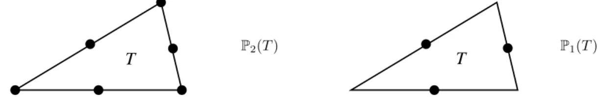
01(Ω) = V and the method is conforming. We could increase the polynomial degree to quadratics P
2(T ), and use vertices and midpoint of edges as degrees of freedom; this has a natural generalization to P
n(T ) for any polynomial degree n ≥ 1 [13, 15, 23]. The resulting method is conforming, namely V
N⊂ V .
T
P
2(T )
T
P
1(T )
Alternatively, we could use affine polynomials P
1(T ), but choose the midpoint of edges as degrees of freedom.
The resulting method, due to Crouzeix and Raviart, is nonconforming, i.e. V
N6⊂ V [13, 15, 17, 35].
We denote by N = N
Nthe set of nodes of T
Nand ˚ N
Nthe interior nodes; then # ˚ N
N= N . We denote by S = S
Nthe set of sides (or faces) of elements of T
N. For each node z ∈ N , we denote by φ
zthe piecewise linear (hat) function with nodal values 1 at z and 0 otherwise; if z ∈ N ˚
Nthen φ
z∈ V
N. The set { φ
z}
z∈N˚forms the canonical basis of V
Nwhereas { φ
z}
z∈Nsatisfies the key property P
z∈N
φ
z(x) = 1 for all x ∈ Ω.
φ z
z
ω z
z
Figure 1.1: Piecewise linear basis function φ
zcorresponding to interior node z, support ω
zof φ
zand scheleton γ
z, the latter being composed of all sides within the interior of ω
z.
1.8 Polynomial Interpolation
If v ∈ W
pm(Ω) with sob(W
pm) > 0 then v is continuous and the Lagrange interpolant is well defined I
Nv(x) = X
z∈NN
v(z)φ
z(x) for all x ∈ Ω.
However, this operator is not adequate for rougher functions such as those in H
1(Ω); see Exercise 2 below.
We will make use of a quasi-interpolant due to Cl´ement [24] and Scott-Zhang [51].
Proposition 1.12 (Quasi-interpolant). Let n ≥ 1 be the polynomial degree, m ≥ 1 be the regularity index, and 1 ≤ p ≤ ∞ be the integrability index. There exists an operator I
N: L
1(Ω) → V
Nsuch that for all v ∈ W
pm(Ω) and T ∈ T
Nwe have
k D
t(v − I
Nv) k
Lq(T). h
sob(Ws
p)−sob(Wqt)
T
k D
sv k
Lp(N(T))(1.24)
where 0 ≤ t ≤ s ≤ min(m, n + 1), sob(W
ps) > sob(W
qt), and N(T ) is a discrete neighborhood of T that includes all elements of T
Nwith nonempty intersection with T. In addition, if m ≥ 1 and the trace of v is 0, then I
Nv also vanishes on ∂Ω.
We point out that if v ∈ C(Ω) and I
Nis the Lagrange interpolation operator, we have a similar estimate to (1.24) with N (T ) = T , that is the estimate is completely local. We also observe that (1.24) does not require the regularity indices t and s to be integer. Combining (1.20) with (1.24) we obtain the following result.
Lemma 1.13 (A priori error estimate). Let 0 ≤ s ≤ n + 1 and u ∈ H
s(Ω) be the solution of the model problem. Let T
Nbe a quasi-uniform partition of Ω with N interior nodes. Let U
N∈ V
Nbe the discrete solution with polynomial degree n ≥ 1. Then
k u − U
Nk
H1(Ω). N
−s/d| u |
Hs(Ω)(1.25) irrespective of n.
Proof. Since T
Nis quasi-uniform, we have h
T≈ N
−1/dfor all T ∈ T
N. The assertion follows from (1.24) for p = q = 2 and t = 1.
Figure 1.2: Sequence of uniform meshes for L-shaped domain Ω
Example 1.1 (Corner singularity). We present 2D numerical experiments on uniform meshes with meshsize h and degrees of freedom N ≈ h
−2for the Dirichlet problem − ∆u = f with exact solution (in polar coordinates)
u(r, θ) = r
23sin(2θ/3) − r
2/4,
on an L-shaped domain Ω; this function satisfies u ∈ H
s(Ω) for s < 2/3. In Figure 1.2 we depict the sequence of uniform meshes, and in Table 1.1 we report the order of convergence for polynomial degrees n = 1, 2, 3.
The asymptotic rate is about h
2/3, or equivalently N
−1/3, regardless of n and is consistent with the estimate (1.25); this also shows that (1.25) is sharp. The situation is strikingly different for graded meshes. We will
h linear (n= 1) quadratic (n= 2) cubic (n= 3)
1/4 1.14 9.64 9.89
1/8 0.74 0.67 0.67
1/16 0.68 0.67 0.67
1/32 0.66 0.67 0.67
1/64 0.66 0.67 0.67
1/128 0.66 0.67 0.67
Table 1.1: The asymptotic rate of convergence for uniform meshes is about h
2/3, or equivalently N
−1/3, as predicted by (1.25) irrespective of the polynomial degree n.
show numerical experiments for graded meshes in Lecture 4 along with a proof of optimal decay rates in
Lecture 5.
1.9 Exercises of Lecture 1
1. Let u(x) = x
γwith 0 < γ < 1 and x ∈ Ω = (0, 1). Let ε > 0 be a given tolerance for max-error:
k u − U
Nk
L∞(Ω)≤ ε. Let N
1and N
2be the degrees of freedom with uniform and graded partition. Show that
(a) γ > 1 ⇒ N
1/N
2≈ γ; (b) γ < 1 ⇒ N
1/N
2= ε
1−1/γ.
Note that for ε = 10
−2and γ = 10
−1, we have N
1/N
2= 10
18. This is the case of checkerboard coefficients A for the model problem in 2d. See § 4.4 of Lecture 4 and [37, 42, 43].
2. Find the weak gradient of
(a) a hat function φ
zin 1d and 2d;
(b) v(x) = log log( | x | /2) in the unit ball.
Note that ∇ φ
z∈ L
∞(Ω) and ∇ v ∈ L
2(Ω) \ L
∞(Ω). So functions in H
1(Ω) may not be continuous, and even bounded, in dimension d ≥ 2.
3. Prove the Poincar´e inequality II
k v k
L2(Ω). diam(Ω) k∇ v k
L2(Ω)for all v ∈ H
01(Ω).
To this end, consider a flat part of ∂Ω contained in R
d−1and write for t > 0 v
2(x, t) = v
2(x, 0) + 2
Z
t 0∂
tv · v for all v ∈ C
∞( ¯ Ω).
Integrate and use Cauchy-Schwarz to prove the inequality for v ∈ C
0∞(Ω). Next use a density argument, based on the definition of H
01(Ω), to extend the inequality to H
01(Ω).
4. Use the same identity as in Exercise 3, followed by a density argument to derive the trace inequality k v k
2L2(∂Ω). diam(Ω)
−1k v k
2L2(Ω)+ diam(Ω) k∇ v k
2L2(Ω)for all v ∈ H
1(Ω).
5. Show that
(a) v ∈ H
−1(Ω) if v ∈ L
2(Ω);
(b) div q ∈ H
−1(Ω) if q ∈ [L
2(Ω)]
d. Compute the corresponding H
−1-norms.
6. (a) Find a variational formulation which amounts to solving
− ∆u = f in Ω, ∂
νu + pu = g on ∂Ω
where f ∈ L
2(Ω), g ∈ L
2(∂Ω), 0 < p
1≤ p ≤ p
2on ∂Ω. Show that the bilinear form is coercive in H
1(Ω).
(b) Suppose that p = ε
−1→ ∞ . What is the boundary value problem satisfied by u
0= lim
ε↓0u
ε? (c) Can you derive an error estimate for k u
0− u
εk
H1(Ω)?
7. Let A be (uniformly) SPD and c ∈ L
∞(Ω) satisfy c ≥ 0. Consider the quadratic functional I[v] = 1
2 Z
Ω
∇ v · A(x) ∇ v + c(x)v
2− h f, v i for all v ∈ H
01(Ω).
Show that u ∈ H
01(Ω) is a minimizer of I[v] if and only if u satisfies the Euler-Lagrange equation B [u, v] =
Z
Ω
∇ v · A ∇ u + c uv = h f, v i for all v ∈ H
01(Ω).
8. The gap in (1.21) is dictated by β/α. Determine this quantity for the Model Problem and (a) k v k
V= | v |
1,Ω; (b) k v k
V=
Z
Ω
∇ v · A ∇ v
1/2.
9. Show that the finite element space V
Nis a subspace of H
01(Ω) of dimension N. Find a local basis (hat functions) and write the discrete problem (1.17) in terms of this basis. Show that the resulting matrix for the model problem is sparse and symmetric positive definite (SPD).
10. Graded mesh: Let u(r, φ) ∼ r
γfor γ < 1 at the origin in 2d. Consider a mesh T such that h
T≈ Λ r
1−γ/2Tfor all T ∈ T
away from 0, where r
T= dist(T, 0) and Λ is a constant. Show that for piecewise linear finite elements (a) N = number of degrees of freedom ≈ R
Ω
h(x)
−2dx ≈ Λ
−2;
(b) k u − U
Nk
H1(Ω)≈ N
−1/2.
Lecture 2 Bisection and Constructive Approximation
In this lecture we discuss bisection as a basic procedure to subdivide elements marked for refinement, and to refine surrounding elements in order to retain conformity (completion process). We show that these additional refinements do not substantially inflate the number of elements. This result is crucial for the following discussion of constructive approximation as well as for Lecture 5 on optimal cardinality of AFEM.
Part 1: The Bisection Method
We follow the work of Binev-Dahmen-DeVore [10] for d = 2, and Stevenson [53] for d > 2. Our emphasis in
§§ 2.1 and 2.2 is the case d = 2, for simplicity, but the complexity analysis of § 2.3 is multidimensional.
2.1 Newest Vertex Bisection
We focus in 2d but the method applies in any dimension (see Stevenson [38, 53, 54]). We consider the newest vertex bisection method (see Mitchell [41]). Given an element T ∈ T
0in the initial partition we mark one of its vertices v(T ) and edge E(T ) opposite to v(T ).
2 2
1 2
1 1
E(T ) T
v(T ) = v(T )
v(T) T
T E(T)
E(T )
The same happens with any element created later. To this end we give a subdivision rule: the element T ∈ T is cut by joining v(T ) and the midpoint of E(T ); this gives rise to two elements T
1, T
2, the children of T , whose vertex v(T
1) = v(T
2) is the midpoint of E(T ) and E(T
1), E(T
2) are the opposite edges to v(T
1), v(T
2).
Lemma 2.1 (Shape regularity). The partitions generated by newest vertex bisection satisfy a uniform min- imal angle condition only depending on T
0, and are thus shape regular.
Proof. Each T ∈ T
0gives rise to a fixed number of similarity classes which, combined with the fact that # T
0is finite, yields the assertion.
Master Forest. Bisection creates a unique master forest F of binary trees with infinite depth, where each node is a simplex (triangle in 2d), its two successors are the two children created by bisection, and the roots of the binary trees are the elements of the initial conforming partition T
0. It is important to realize that, no matter how an element arises in the subdivision process, its associated newest vertex is unique and only depends on the labeling of T
0: so v(T ) and E(T ) are independent of the order of the subdivision process for all T ∈ F ; see Lemma 2.3 below. Therefore, F is unique.
A finite subset F ⊂ F is called a forest if T
0⊂ F and the nodes of F satisfy (a) all nodes of F \ T
0have a predecessor;
(b) all nodes in F have either two successors or none.
Any node of F is thus uniquely connected with a node of the initial triangulation T
0. Furthermore, any forest
may have interior nodes, i.e. nodes with successors, as well as leaf nodes, i.e. nodes without successors. The
set of leaves corresponds to a subdivision (or triangulation, mesh, partition) T = T ( F ) of T
0.
If F ⊂ F
∗are two forests, we call T
∗= T ( F
∗) a refinement of T = T ( F ) and denote it T
∗≥ T . We define R = R
T →T∗:= T \ ( T
∗∩ T )
as the set of refined elements, i.e. R is the set of leaves of F that are interior nodes of F
∗. The class of conforming refinements by bisection of T
0is
T = {T ( F ) | F ⊂ F and T ( F ) is conforming } , and
T
N= {T | T ∈ T and # T − # T
0≤ N } .
The level (or generation) ℓ(T ) of an element T ∈ T is the number of ancestors it has in F or, equivalently, the number of bisections needed to create T from T
0. Therefore ℓ(T ) = 0 for all T ∈ T
0. In view of Lemma 2.1, we see that h
T= diam(T ) ≈ | T |
1/2and deduce the following geometric property.
Lemma 2.2 (Element diameter). There exists constants 0 < D
1< D
2only dependent on T
0such that D
12
−ℓ(T)/2≤ h
T≤ D
22
−ℓ(T)/2for all T ∈ T .
Proof. Exercise 3.2.
Chains. In order to study nonlocal effects of bisection we introduce now the concept of chain. To each T ∈ T we associate the element F (T ) ∈ T sharing the edge E(T ) if E(T ) is interior and F (T ) = ∅ if E(T ) is on ∂Ω. A chain C (T ), with starting element T ∈ T , is a sequence { T, F (T ), . . . , F
m(T ) } with no repetitions of elements and with
F
m+1(T ) = F
k(T ) for k ∈ { 0, . . . , m − 1 } or F
m+1(T ) = ∅ .
Two adjacent elements T, T
′= F (T ) are compatibly divisible (or T, T
′form a compatible bisection patch) if F (T
′) = T . Hence, C (T ) = { T, T
′} and a bisection of either T or T
′does not propagate outside the patch.
11 9
10 1
2 3
4
2 3
5 6
7
8
2 3
5
8 12
T T
T T
T T
T
T T
T T T T
T T
T
T T
T
1T
2T
3T
11T
12T
5T
T
64
T
7T
8T
10T
9Examples (Chains). Let F = { T
i}
12i=1be the forest in the figure above. Then C (T
6) = { T
6, T
7} , C (T
9) = { T
9} ,
and C (T
10) = { T
10, T
8, T
2} are chains, but only C (T
6) is a compatible bisection patch.
Labeling of Edges. To study the structure of chains it is convenient to label edges of T . Given T ∈ T with level ℓ(T ) = i, we assign the label (i + 1, i + 1, i) to T with i corresponding to the refinement edge E(T ). The following rule dictates how the labeling changes with refinement: the side i is bisected and both new sides as well as the bisector are labeled i + 2 whereas the remaining labels do not change (see the figure below).
0
0
0 0
0 0
0
0 1 1
1 1
1 1 1
1
1
1 1
2 2
2 2
2 2
2
2
2 2
2 2
3 3
3 3
To guarantee that the label of an edge is independent of the elements sharing this edge, we need a special labeling for T
0: edges of T
0have labels 0 or 1 and all elements T ∈ T have exactly two edges with label 1 and one with label 0. It is not obvious that such a labeling exists.
Remark 2.1 (Initial labeling). Given a coarse mesh of elements T we can bisect twice each T and label the 4 grandchildren, as indicated in the figure below, for the resulting mesh T
0to satisfy the initial labeling [10].
A similar, but much trickier, construction can be done in any dimension d > 2 (see Stevenson [53]).
1 1 1 1
1
1
1 0
0
2.2 Properties of Bisection
Given T ∈ T and a subset M ⊂ T of marked elements, we now study the procedure T
∗= REFINE ( T , M )
that refines all elements of M , and perhaps additional elements, so that T
∗≥ T is conforming.
Lemma 2.3 (Labeling). Let T
0≤ T
1≤ · · · ≤ T
nbe generated by REFINE with the edge labeling and initial labeling of T
0stated above. Then each side in T
khas a unique label independent of the two triangles sharing this edge.
Proof. We argue by induction. For k = 0 the assertion is valid due to the initial labeling. Suppose the
statement is true for T
k. An edge S in T
k+1can be obtained in two ways. The first is that S is a bisector,
and so a new edge, in which case there is nothing to prove about its label being unique. The second possibility
is that S was obtained by bisecting an edge S
′∈ S
k. Let T, T
′∈ T
kbe the elements sharing S
′, and let us
assume that E(T
′) = S
′. Let (i + 1, i + 1, i) be the label of T
′, which means that S is assigned the label
i + 2. By induction, the label of S
′as an edge of T is also i. There are two possible cases for the label of T :
• Label (i + 1, i + 1, i): this situation is symmetric, E(T ) = S
′, and S
′is bisected with both halves getting label i + 2.
i +1
i +1
i +1
i +1
i +1
i +1
i +1
i +1
i +2
i +2
i +2
i +2
T
T ’ i
’= E(T
S ’) = E(T )
• Label (i, i, i − 1): a bisection of side E(T ) with label i − 1 creates a children T
′′with label (i+1, i+1, i) that is compatibly divisible with T
′. Joining the new node of T with the midpoint of S
′creates a conforming partition with level i + 2 assigned to S.
i
+1i
+1i
+1i
+1i
+1T ’ T ’
i
+1T ’’
i
+1i
+1i
+1i
+1i
+1i
+2i
+2i
+2i
+2i
+1T
i i
i i
−1i i
Therefore, in both cases the label i + 2 assigned to S is the same from both sides, as asserted.
Corollary 2.4 (Consecutive element levels). For any T ∈ T and T, T
′= F(T ) ∈ T we have:
(a) ℓ(T ) = ℓ(T
′) and T, T
′are compatibly divisible, or
(b) ℓ(T
′) = ℓ(T ) − 1 and T is compatibly divisible with a child of T
′.
Corollary 2.5 (Element levels on a chain). For all T ∈ T and T ∈ T , its chain C (T ) = { T
k}
mk=0with T
k= F
k(T ) have the property
ℓ(T
k) = ℓ(T ) − k 0 ≤ k ≤ m − 1
and T
m= F
m(T ) has generation ℓ(T
m) = ℓ(T
m−1) or it is a boundary element with lowest labeled edge on
∂Ω. In the first case, T
m−1and T
mare compatibly divisible.
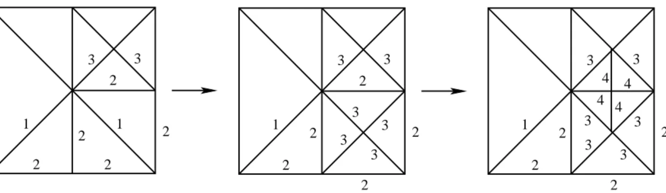
Within the module REFINE we consider the procedure T
∗= refine ( T , T )
which recursively refines the chain C (T ) of T and creates a minimal conforming partition T
∗≥ T . We denote by C (T ) ⊂ T
∗the recursive refinement of T (or completion of C (T )). We refer to the figure below for recursive bisection C (T
10) of T
10. The module REFINE calls refine for all T ∈ M .
Lemma 2.6 (Distance). Let T ∈ M . Any newly created T
′∈ T
∗by refine ( T , T ) satisfies d(T
′, T ) = inf
x′∈T′,x∈T
| x
′− x | ≤ D
22 √
√ 2
2 − 1 2
−ℓ(T′)/2.
3
1 2
3 2
2
2 2
1
3
1 2
3
2
2 2
3 3 3
3 4 4 4
4 3
1 2
3 2
2
2 2
3 3
3 3
Figure 2.1: Recursive refinement of T
10by refine . This entails refining the chain C (T
10) = { T
10, T 8, T
2} . Proof. Suppose T
′⊂ T
i∈ C (T ) have been created by bisectioning of T
i(see figure below). Then
d(T
′, T ) ≤ d(T
i, T ) + diam(T
i) ≤ X
i k=1diam(T
k)
≤ D
2X
i k=12
−ℓ(Tk)/2< D
21
1 − 2
−1/22
−ℓ(Ti)/2,
because the levels decrease exactly by 1 along the chain C (T ) according to Corollary 2.4(b). Since T
′is a child or grandchild of T
i, we deduce ℓ(T
′) ≤ ℓ(T
i) + 2, whence
d(T
′, T ) < D
22 √
√ 2
2 − 1 2
−ℓ(T′)/2. This is the desired estimate.
000000 000000 000000 111111 111111 111111
T ’
0
5
=T
1
2
3
4
T
iT T
T
T T
T
Lemma 2.7 (Level). Let T ∈ M and T
′∈ T
∗be an element newly created by T
∗= refine ( T , T ). Then ℓ(T
′) ≤ ℓ(T ) + 1.
Proof. This is a consequence of Corollary 2.5 and the fact that refine ( T , T ) creates children of T and either children or grandchildren of triangles T
k∈ C (T ) = { T
i}
mi=0with k ≥ 1. If T
′is a child of T there is nothing to prove. If not, we consider first m = 1, in which case T
′is a child of T
1because T
0and T
1are compatibly divisible and so have the same level; thus ℓ(T
′) = ℓ(T
1) + 1 = ℓ(T
0) + 1. Finally, if m > 1, then apply Corollary 2.5 to deduce
ℓ(T
′) ≤ ℓ(T
k) + 2 ≤ ℓ(T ) + 1,
as asserted.
2.3 Complexity of REFINE
We would like to show that REFINE does not inflate the number # M of marked elements M . However, the most obvious statement
# T
∗− # T ≤ Λ # M
is not correct with a constant Λ independent of the level of refinement. For an example we refer to the bisection of C (T
10) as shown in Figure 2.1; the chain C (T
10) has as many elements as the level ℓ(T
10) of T
10. Heuristics. Consider the set M = S
n−1k=0
M
kused to generate T
n≥ T
n−1≥ · · · ≥ T
1. Suppose that each element T
′∈ M is assigned a fixed amount C
1of dollars to spend on refined elements. Each such T
′invests money on new elements in such a way that each T ∈ T
n\ T
0gets at least a fixed amount C
2. If λ(T, T
′) is the portion of money spent by T
′∈ M on T ∈ T
n\ T
0, then
X
T∈Tn\T0
λ(T, T
′) ≤ C
1, X
T′∈M
λ(T, T
′) ≥ C
2.
Therefore
C
2(# T
n− # T
0) ≤ X
T∈Tn\T0
X
T′∈M
λ(T, T
′) = X
T′∈M
X
T∈Tn\T0
λ(T, T
′) ≤ C
1# M . The construction of such an allocation function is the chief objective of this section.
Construction of λ(T , T
′). Let { a(k) }
∞k=−1, { b(k) }
∞k=0be sequences satisfying X
∞k=−1
a(k) < ∞ , X
∞ k=0b(k) 2
−k/2< ∞ , inf
k≥0
b(k)a(k) > 0;
for instance we could take a(k) = (k + 2)
−2and b(k) = 2
k/4. Let A := D
21 + 2 √
√ 2 2 − 1
X
∞k=0
b(k) 2
−k/2.
Let T = T
nand define λ : T × M → R
+by λ(T, T
′) =
( a(ℓ(T
′) − ℓ(T )) if d(T, T
′) < A 2
−ℓ(T)/2and ℓ(T ) ≤ ℓ(T
′) + 1
0 otherwise.
Therefore, the investment of T
′∈ M is restricted to cells T with level at most ℓ(T
′) + 1.
Lemma 2.8 (Upper bound). There exists a constant C
1> 0 only depending on T
0such that X
T∈T \T0
λ(T, T
′) ≤ C
1for all T
′∈ M .
Proof. Given T
′∈ M and k ≥ 0, the number of elements T ∈ T satisfying ℓ(T ) = k and d(T, T
′) < A 2
−k/2is uniformly bounded because of Lemma 2.2 (recall that h
T≥ 2
−ℓ(T)/2). Therefore
X
T∈T \T0
λ(T, T
′) .
ℓ(T′)+1
X
k=0
a(ℓ(T
′) − k) . X
∞ k=−1a(k),
which is the desired upper bound.
Lemma 2.9 (Lower bound). There exists a constant C
2> 0 only depending on T
0such that X
T′∈M
λ(T, T
′) ≥ C
2for all T ∈ T \ T
0.
Proof. Let T
0∈ T \ T
0be fixed, and let { T
j}
sj=1⊂ M be a set of marked elements so that T
jhas been created by a call of refine to bisect T
j+1. In view of Lemma 2.7
ℓ(T
j+1) ≥ ℓ(T
j) − 1,
so ℓ(T
j+1) can only decrease by 1 the previous value of ℓ(T
j). Since the sequence eventually ends with T
j∈ T
0, and so ℓ(T
j) = 0, there exists a smallest value s such that
ℓ(T
s) = ℓ(T
0) − 1.
Moreover, for 1 ≤ j ≤ s we have
d(T
0, T
j) ≤ d(T
0, T
1) + diam(T
1) + d(T
1, T
j)
≤ X
j k=1d(T
k−1, T
k) +
j−1
X
k=1
diam(T
k), and applying Lemmas 2.2 and 2.6, we obtain
d(T
0, T
j) ≤ D
22 √
√ 2 2 − 1
X
j k=12
−ℓ(Tk−1)/2+ D
2 j−1X
k=1
2
−ℓ(Tk)/2= D
21 + 2 √
√ 2 2 − 1
j−1X
k=0
2
−ℓ(Tk)/2= D
21 + 2 √
√ 2 2 − 1
X
∞i=0
m(i, j) 2
−(ℓ(T0)+i)/2where m(i, j) denotes the number of k ≤ j − 1 with
ℓ(T
k) = ℓ(T
0) + i.
We need to distinguish two cases depending on the size of m(i, s).
Case 1: m(i, s) ≤ b(i) for all i ≥ 0. We see that d(T
0, T
s) < D
21 + 2 √
√ 2 2 − 1
X
∞i=0