Growth and the Ageing Joneses

IHS Economics Series Working Paper 230

November 2008

Growth and the Ageing Joneses

Walter H. Fisher

Ben J. Heijdra

Impressum Author(s):

Walter H. Fisher, Ben J. Heijdra Title:

Growth and the Ageing Joneses ISSN: Unspecified

2008 Institut für Höhere Studien - Institute for Advanced Studies (IHS) Josefstädter Straße 39, A-1080 Wien

E-Mail: o ce@ihs.ac.atffi Web: ww w .ihs.ac. a t

All IHS Working Papers are available online: http://irihs. ihs. ac.at/view/ihs_series/

This paper is available for download without charge at:

https://irihs.ihs.ac.at/id/eprint/1876/

Growth and the Ageing Joneses

Walter H. Fisher, Ben J. Heijdra

230

Reihe Ökonomie

Economics Series

230 Reihe Ökonomie Economics Series

Growth and the Ageing Joneses

Walter H. Fisher, Ben J. Heijdra November 2008

Institut für Höhere Studien (IHS), Wien

Institute for Advanced Studies, Vienna

Contact:

Walter H. Fisher

Department of Economics and Finance Institute for Advanced Studies Stumpergasse 56

1060 Vienna, Austria : +43/1/599 91-253 Fax: +43-159991-555 email: fisher@ihs.ac.at

Ben J. Heijdra

Department of Economics University of Groningen P.O. Box 800

9700 AV Groningen, The Netherlands email: b.j.heijdra@heijdra.org and

Institute for Advanced Studies, Netspar, CESifo

Founded in 1963 by two prominent Austrians living in exile – the sociologist Paul F. Lazarsfeld and the economist Oskar Morgenstern – with the financial support from the Ford Foundation, the Austrian Federal Ministry of Education and the City of Vienna, the Institute for Advanced Studies (IHS) is the first institution for postgraduate education and research in economics and the social sciences in Austria.

The Economics Series presents research done at the Department of Economics and Finance and aims to share “work in progress” in a timely way before formal publication. As usual, authors bear full responsibility for the content of their contributions.

Das Institut für Höhere Studien (IHS) wurde im Jahr 1963 von zwei prominenten Exilösterreichern – dem Soziologen Paul F. Lazarsfeld und dem Ökonomen Oskar Morgenstern – mit Hilfe der Ford- Stiftung, des Österreichischen Bundesministeriums für Unterricht und der Stadt Wien gegründet und ist somit die erste nachuniversitäre Lehr- und Forschungsstätte für die Sozial- und Wirtschafts- wissenschaften in Österreich. Die Reihe Ökonomie bietet Einblick in die Forschungsarbeit der Abteilung für Ökonomie und Finanzwirtschaft und verfolgt das Ziel, abteilungsinterne Diskussionsbeiträge einer breiteren fachinternen Öffentlichkeit zugänglich zu machen. Die inhaltliche Verantwortung für die veröffentlichten Beiträge liegt bei den Autoren und Autorinnen.

Abstract

We incorporate Keeping-up-with-the-Joneses (KUJ) preferences into the Blanchard-Yaari (BY) framework and develop, using an AK technology, a model of balanced growth. In this context we investigate status preference, demographic, and pension policy shocks. We find that a higher degree of KUJ lowers economic growth, while, in contrast, a decrease in the fertility and mortality rates increase it. In the second part of the paper we extend the model by incorporating a Pay-as-you-go (PAYG) pension system with a statutory retirement date.

This introduces a life-cycle in human wealth earnings and implies that the growth rate is higher under PAYG. We also consider the implications of an increase in the retirement date under both defined benefit and defined contribution schemes.

Keywords

Relative consumption, OLG, endogenous growth, pension reform

JEL Classification

D91, E21, H55

Comments

The authors would like to thanks Jochen Mierau and Ward Romp for helpful comments.

Contents

1 Introduction 1

2 The Macroeconomy 3

2.1 Firms... 3 2.2 Households... 4

3 Aggregation and the Macroeconomic Equilibrium 5

4 Steady-State Growth 7

5 Comparative Static Effects 9 6 Introducing a PAYG Pension System 11 7 Pension Policy and Economic Growth 14

8 Conclusions 17

Appendix A: Derivation of equations (16)–(17) 19 Appendix B: Conditions on steady-state profiles 20 Appendix C: Derivation of (46) and (47) 22 Appendix D: PAYG and the welfare of newborns 23

References 23

1 Introduction

Since the 1980s one of the main streams of research investigating the conditions for sustained economic growth has viewed the accumulation of capital, broadly measured, as one of its key sources. This approach, often termed the “AK” framework, has been propagated, among others, by authors such as Romer (1986), Barro (1990), and Rebelo (1991). In its canonical, single-factor form, the AK model yields a constant balanced growth rate with no transitional dynamics. In contrast to the standard Solow model, tax and government infrastructure pol- icy (see Barro, 1990) affects the growth rate by changing the rate of return on capital.

The studies cited above all employ the representative agent (RA) framework. In this pa- per we seek to extend the insights of the AK setting by adopting the overlapping generations (OLG) approach to specifying the consumer sector. Specifically, we use the Blanchard (1985)- Yaari (1965) continuous-time framework to model the decisions of finite-lived consumers. A central characteristic of the Blanchard-Yaari (BY) model is the demographic turnover from old to young population cohorts. Since the asset-poor young replace the asset-rich old in this setting, demographic turnover influences the economy’s saving and, thus, its accumula- tion of capital. A key advantage, then, of the BY framework is that it enables us to consider how demographic parameters influence economic growth in the AK context in which capital accumulation plays the decisive role. Since population dynamics obviously depends on fac- tors such as birth and mortality rates, we can use our model to investigate how demographic shocks affect the balanced growth rate.

Due to its well-defined population dynamics, we can use the BY model to investigate the effects of public policies, in particular, Pay-as-you-go (PAYG) pensions, that have a significant intergenerational component.

Another important property of the BY framework, as recently shown by Fisher and Heij dra (2008) in an exogenous growth setting, is that the importance of demographic turnover also depends on agents’ preferences, specifically on their attitude to status. In our endoge- nous growth framework, this allows us to ask the question whether or not status compe- tition is an engine of economic growth. Recent authors who investigate this issue using an endogenous growth, representative agent (RA) framework that specifies consumption as the reference good include Alvarez-Cuadrado et al. (2004), Liu and Turnovsky (2005), and Turnovsky and Monteiro (2007). The specification used by these authors is often termed the

“Keeping up with the Joneses” (KUJ) specification of status preferences.

This literature does

1In non-endogenous growth contexts, recent authors who employ the BY framework to consider the effects of demographic shocks include Heijdra and Ligthart (2006) and Bettendorf and Heijdra (2006), the latter employing a small open economy framework. In this research demographic shocks are time-dependent, though cohort independent, an approach we follow here.

2Strictly speaking, the Alvarez-Cuadradoet al. (2004) and Turnovsky and Monteiro (2007) employ a “Catch-

1

not, however, deliver an unambiguous answer regarding whether or not status competition is growth-promoting. Indeed, the relationship between status and growth in this context is highly sensitive to the specification of preferences and technology.

The RA model is, moreover, a restrictive one to analyze the implications of status prefer- ences, since all agents end up with the same consumption and asset holdings in the symmet- ric equilibrium, a situation implying that no one wins the “rat race”. In contrast, agents of different ages, or “vintages”, in the OLG framework possess distinct stocks of wealth and en- joy distinct levels of consumption. An economy-wide shift in KUJ then has age-dependent effects in the OLG context. A framework in which differences among individuals persist over time is, we believe, a promising avenue to explore the macroeconomic implications of status competition. Another important task in this paper, then, is to extend the findings of Fisher and Heijdra (2008) to the endogenous growth context and to consider the implications of changes in the degree of status preference.

Among our results, we show that the balanced growth rate, due to intergenerational turnover in financial wealth, is lower in the BY framework compared to its RA counter- part. We also consider demographic disturbances characteristic of advanced societies; falls in fertility and rises in longevity. In this context we find that while a decline in fertility and a rise in longevity both increase the growth rate, they have opposite implications for the consumption-capital ratio: the latter rises in response to a “baby bust” and falls subsequent to a jump in life-expectancy. Furthermore, we show that an increase in the degree of sta- tus preference lowers economic growth, since generational turnover, which tends to reduce growth, becomes more important in this scenario. Finally, in the second part of the paper, we investigate the implications of incorporating a PAYG pension system, featuring an ex- ogenous retirement date. We find that economic growth is higher, given our design of the scheme, under PAYG. Again, it is demographic turnover that provides the source for this result. Specifically, PAYG pensions introduce a ‘wedge’ between the human wealth of new- borns and the average stock of human wealth. Since newborns possess more human wealth than older agents under the PAYG system, the intergenerational turnover in human wealth provides a countervailing element to the turnover in financial wealth, which, as indicated, lowers economic growth in the BY framework.

ing up with the Joneses” approach in which reference consumption depends on past consumption and evolves over time.

3Alvarez-Cuadradoet al. (2004) find that the role of reference consumption in determining the response to macroeconomic shocks depends on whetherAKor the more flexible Cobb-Douglas technology is assumed. In Liu and Turnovsky (2005) the effect of KUJ on balanced growth is a function of the intertemporal elasticity of sub- stititution. Turnovsky and Monteiro (2007) show that consumption externalities affect the long-run equilibrium if and only if work effort is endogenous.

2

The paper is organized as follows. Section 2 outlines the firm and household sectors of the economy, which are aggregated in section 3 to determine the macroeconomic equilib- rium. Section 4 derives the balanced rate of endogenous growth, while section 5 investigates how the latter is influenced by demographic and status preference shocks. Section 6 intro- duces the PAYG system into our OLG framework, which we analyze in section 7. There, we consider, first, the effect of public pensions on the rate of growth and, second, how an increase in the statutory retirement age influences the growth rate in both defined benefit and defined contribution schemes. We close in section 8 with brief concluding remarks and include an appendix containing supporting mathematical results.

2 The Macroeconomy

2.1 Firms

We begin by first analyzing the economy’s firm sector. This permits us to describe the engine of endogenous growth, which relies, in the spirit of Romer (1989) and Saint-Paul (1992), on an inter-firm externality. The latter also leads to a constant (real) interest rate, a result that simplifies the derivation of the macroeconomic equilibrium. The firm sector is made up of a large number of perfectly competitive firms producing a homogenous good. At the individual firm level, output technology is Cobb-Douglas:

Y

( t ) = F [ K

( t ) , L

( t )] ≡ Z ( t ) · K

( t )

L

( t )

, 0 < ε < 1, (1) where Y

( t ) represents net output

of firm i, K

( t ) is the capital stock, L

( t ) is labor supply (coinciding here with the population), and Z ( t ) is total factor productivity common to all firms. For simplicity, we assume that capital accumulation does not incur adjustment costs.

As usual under profit maximization, the rental values of capital and labor correspond to their marginal physical products:

w ( t ) = ^∂Y

( t )

∂L

( t ) = ( 1 − _ε ) Z ( t ) · _k

( t )

, r ( t ) = ^∂Y

( t )

∂K

( t ) = εZ ( t ) · _k

( t )

, (2) where k

( t ) ≡ K

( t ) /L

( t ) is the capital-labor ratio. Moreover, since each firm faces the same wage rate and rental rate of capital, each has the same capital-labor ratio, k

( t ) = k ( t ) , which implies that firm output corresponds to Y

( t ) = Z ( t ) L

( t ) k

( t ) . To obtain economy-wide relationships, we define: Y ( t ) ≡ ∑

Y

( t ) , K ( t ) ≡ ∑

K

( t ) , and L ( t ) ≡ ∑

L

( t ) . In turn, the inter-firm externality is given by:

Z ( t ) = Z

· k ( t )

, Z

> 0, (3)

4That is, net output incorporates capital stock depreciation

3

which implies that individual firms in this setting benefit from a rise in the average capital intensity. Aggregating firm output and substituting for Z ( t ) = Z

· k ( t )

, we obtain the linear-in-capital, economy-wide production function Y ( t ) = Z

K ( t ) . Substituting Z ( t ) = Z

· k ( t )

into the marginal productivity conditions (2), we calculate expressions for the wage and the interest rate:

w ( t ) = ( 1 − _ε ) y ( t ) = ( 1 − _ε ) Z

k ( t ) , r ( t ) = r = εZ

> _{0. (4)} Clearly, the interest rate is a positive constant, a result that is the source of continued growth.

In contrast, agents can look forward to ongoing wage growth in this setting.

2.2 Households

We assume that the economy consists of agents of different birth dates, or “vintages”, who compare their own consumption ¯ c ( v, τ ) to the average level of consumption c ( τ ) . Following Fisher and Heijdra (2008), for a consumer born at time v (v ≤ t) lifetime utility at t equals:

Λ ( v, t ) =

Z ∞

t

ln ¯ x ( v, τ ) e

dτ, (5)

where ρ is the rate of time preference, β is the given instantaneous death probability (inde- pendent of age), and ¯ x ( v, τ ) is the instantaneous subfelicity function defined as:

¯

x ( v, τ ) ≡ ^{c ¯} ( v, τ ) − αc ( τ )

1 − α , α < 1, (6)

where the parameter α determines the agent’s attitude to status competition. If 0 < α < 1, agents exhibit jealousy of the consumption of others. On the other hand, if α < 0, then agents express admiration for the consumption of others. The preferences in (6) satisfy the conditions for “Keeping up with the Joneses” (KUJ).

The budget identity of an agent born at time v equals:

˙¯

a ( v, τ ) = ( r + β ) a ¯ ( v, τ ) + w ( τ ) − c ¯ ( v, τ ) , (7) where ¯ a ( v, τ ) represents assets, r is the fixed interest rate, and w ( τ ) is the cohort-independent wage rate earned by agents who supply one unit of work effort. Assets yield an annuity in- come of ( r + β ) a ¯ ( v, τ ) , which consists of interest payments r a ¯ ( v, τ ) and annuity receipts β a ¯ ( v, τ ) . Employing the usual methods of optimal control, we calculate the following time- profile for ¯ x ( v, τ ) :

˙¯

x ( v, τ )

¯

x ( v, τ ) = r − ρ, r > ρ. (8)

5KUJ is satisfied withU[·]≡lnx(v,τ), since∂²U[·]/∂¯c∂c =c/(c−αc¯)²>0. See Dupor and Liu (2003) and Liu and Turnovsky (2005) for a detailed characterization of relative consumption preferences.

4

The necessary condition r > ρ implies that we focus on a given rising profile of ¯ x ( v, τ ) . In (8) we also obtain the usual BY-result that the probability of death β cancels out along individual time-profiles, since the (higher) annuity rate of return r + β is offset by the (greater) effec- tive rate of time preference ρ + β.

In fact, at the aggregate level, the crucial demographic parameter (see (16) below) is the fertility rate, denoted by η.

The next step is to calculate the intertemporal budget constraint of the individual. Inte- grating (7) subject to the NPG condition lim

a ¯ ( v, τ ) e

= 0, yields:

Z ∞

t

[( 1 − α ) x ¯ ( v, τ ) + αc ( τ )] e

dτ = a ¯ ( v, t ) + h ( t ) , (9) where h ( t ) = R

t

w ( τ ) e

dτ is age-independent human wealth.

Equation (9) states that the present discounted value of a weighted average of individual subfelicity and av- erage consumption — where the weights depend on the parameter α — corresponds to the aggregate of the agent’s financial and human wealth. Integrating (8) to obtain ¯ x ( v, τ ) =

¯

x ( v, t ) e

, τ ≥ t, we can show that (9) reduces to:

( 1 − α ) ^{x ¯} ( v, t )

ρ + β = a ¯ ( v, t ) + h ( t ) − α Γ ( t ) , (10) where Γ ( t ) ≡ R

t

c ( τ ) e

dτ. Substitution of ¯ x ( v, t ) from (6) in (10), yields an ex- pression for individual consumption that is a function of average consumption as well as wealth:

c ¯ ( v, t ) = ( ρ + β ) [ a ¯ ( v, t ) + h ( t )] + α [ c ( t ) − ( ρ + β ) ^Γ ( t )] . (11) Among the features that emerge from (11) is that individual consumption depends on aver- age consumption, due to the existence of a consumption externality, i.e., α 6= 0. Otherwise, an agent consumes — as in the standard setting — out of his wealth according to ρ + β, the marginal propensity to consume.

3 Aggregation and the Macroeconomic Equilibrium

In this section of the paper we first specify the economy’s demography. This is necessary to aggregate the individual relationships and, thus, to describe the OLG macroeconomy.

Letting η represent the birth rate, the (constant) population growth rate is n ≡ η − β, with β,

6Neverthless, thelevelof an agent’s consumption does depend onβ.

7Observe that in a growth context in which wages follow the pathw(τ) =w(t)e^γ(τ−t)ˆ (where the growth rate ˆ

γis determined in section 4), human wealth depends on time,t, but not on the agent’s age,t−v. In contrast, human wealth will be both time- and age-dependent once we introduce a PAYG system in section 6 below.

5

as indicated, the mortality probability. Through time, individual population cohorts L ( v, t ) shrink as their members die off. The population proportion of cohort v at time t thus equals:

l ( v, t ) ≡ ^L ( v, t )

L ( t ) = ηe

, t ≥ v, (12)

which enables us to define the per-capita average values of consumption and financial assets:

c ( t ) ≡

Z _t

−∞

l ( v, t ) c ¯ ( v, t ) dv, a ( t ) ≡

Z _t

−∞

l ( v, t ) a ¯ ( v, t ) dv, (13) where c ( t ) represents, furthermore, the consumption externality from the individual’s point of view. Aggregating individual consumption (11), we obtain:

c ( t ) = ( ρ + β ) [ a ( t ) + h ( t )] + α [ c ( t ) − ( ρ + β ) ^Γ ( t )] . (14) Subtracting (14) from (11), we find:

¯

c ( v, t ) − _c ( t ) = ( ρ + β ) [ a ¯ ( v, t ) − _a ( t )] , (15) where the difference between individual and average consumption depends on the differ- ence between individual and average financial wealth, a fact we use below to draw the distinctions between the BY and RA frameworks.

The key step to derive the growth equilibrium is to obtain the differential equations for average consumption and financial assets, ˙ c ( t ) and ˙ a ( t ) . The details of this exercise are given in Appendix A. Using the expressions for ˙ c ( t ) and ˙ a ( t ) , the rate of return and aggregate relationships of the production sector, and the fact that only physical capital is used for savings, k ( t ) ≡ a ( t ) , we derive the following macroeconomic equilibrium:

c ˙ ( t )

c ( t ) = r − ρ − ^η ( ρ + β ) 1 − α · ^k ( t )

c ( t ) ^{, (16)}

k ˙ ( t ) = [ r − n ] k ( t ) + w ( t ) − c ( t ) , (17)

w ( t ) = ( 1 − ε ) y ( t ) , r = εZ

, (18)

y ( t ) = Z

k ( t ) . (19)

The dynamics of consumption is described by (16), while (17) governs the accumulation of physical capital, n ≡ η − β. Equation (18) reiterates the expressions for the wage and the interest rate, while (19) is the per-capita version of the production function. In contrast to equations (17)–(19), which emerge in the usual Ramsey framework, equation (16) for con- sumption dynamics merits additional comment. The third term on the right-hand-side of (16) is typical in the BY-setting and represents the effect that demographic turnover has on

6

consumption dynamics and, as we show below, economic growth. To see this, we evalu- ate (15) at v = t and impose k ( t ) ≡ a ( t ) . This yields c ( t ) − c ¯ ( t, t ) = ( ρ + β ) k ( t ) , which, if substituted in (16), results in the following alternative representation of ˙ c ( t ) /c ( t ) :

˙ c ( t )

c ( t ) = r − ρ − ^η

1 − α · ^c ( t ) − c ( t, t )

c ( t ) ^{. (20)}

The term [ c ( t ) − c ¯ ( t, t )] , corresponding to the difference between average and new-born con- sumption, measures the effect of intergenerational turnover. In the BY-framework older generations are replaced by newborns. Because, however, agents are born with no financial wealth, their consumption levels fall short of that of their older counterparts. Consequently, the replacement of asset-rich by asset-poor population cohorts reduces the growth rate of av- erage consumption. This is the case even though the growth rate of individual consumption,

˙¯

c ( v, τ ) / ¯ c ( v, τ ) , is the same for each generation facing the given interest rate r.

4 Steady-State Growth

In this model the single accumulable factor of production, physical capital, has the constant returns to scale property. Consequently, the long-run equilibrium is characterized by a sus- tained, balanced growth rate, denoted by ˆ γ. Furthermore, the economy exhibits no transi- tional dynamics. To see why this is the case, let x ( t ) ≡ _c ( t ) /k ( t ) represent the consumption- capital ratio and employ (16)–(19) to derive ˙ x ( t ) /x ( t ) :

˙ x ( t )

x ( t ) = [ r − ρ + Z

− n ] + x ( t ) − ^η ( ρ + β ) 1 − _α · ¹

x ( t ) ^{. (21)}

It is straightforward to show that (21) is an unstable differential equation. Consequently, a stable equilibrium is achieved only if the consumption-capital ratio attains a constant value, x ( t ) ≡ x, ˆ ∀ t ≥ 0, which, in turn, implies that the economy grows at the rate ˆ γ through time. The resulting steady-state growth profiles of capital, wages, and consumption are k ˆ ( t ) = k ^ˆ

e

, ˆ w ( 0 ) = w ˆ

e

, and ˆ c ( t ) = c ˆ

e

, where ˆ k ( 0 ) = k ^ˆ

, ˆ w ( 0 ) = w ˆ

, and ˆ c ( 0 ) = c ˆ

denote their respective initial values.

To determine the solution for the balanced growth rate, we evaluate (16)–(17) along the steady-state profile:

ˆ

γ = r − ρ − ^η ( ρ + β ) 1 − _α

1

x ˆ , γ ˆ = r + ( 1 − ε ) Z

− n − x, ˆ (22) where ˆ x ≡ c/ˆ ˆ k is the consumption-capital ratio. To further simplify the problem, we define the growth-adjusted interest rate as ˆ r

≡ _r − _{γ ˆ} and re-express (22) as:

ˆ r

− ρ

ˆ

x = ^η ( ρ + β )

1 − α , x ˆ = r ˆ

+ ( 1 − ε ) Z

− n. (23)

7

0 0.05 0.1 0.15 0.2 0.25 0.3 0.35 0.4

−0.04

−0.03

−0.02

−0.01 0 0.01 0.02 0.03 0.04

E1

EE CA BY EERA

α = 0.5 α = −0.5

consumption−capital ratio

growth rate

Figure 1: Growth and the KUJ effect Combining the relationships in (23), we form the polynomial Φ ( s ) :

Φ ( s ) ≡ ( s − _ρ ) · [ s + ( 1 − _ε ) Z

− _n ] − ^η ( ρ + β )

1 − α , (24)

where Φ ( r ˆ

) = 0 solves for the growth-adjusted interest rate ˆ r

. There is only one feasible solution with ˆ x > 0. This is satisfied with ˆ r

≡ r − γ ˆ > ρ and ˆ r

> n − ( 1 − ε ) Z

.

The Euler and market clearing relationships can also be combined to determine the polynomial Γ ( s ) that solves for the consumption-capital ratio, i.e., Γ ( x ˆ ) = 0:

Γ ( s ) ≡ s

− [ ρ + ( 1 − ε ) Z

− n ] s − ^η ( ρ + β )

1 − α . (25)

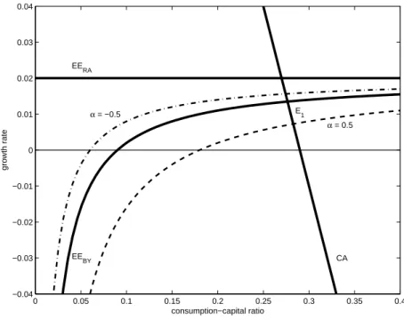
Using (22), we illustrate in Figure 1 the OLG balanced growth equilibrium. The positively- sloped locus EE

represents the Euler equation, while the downward-sloping line CA de- picts market clearing. The relationships (both solid) have the following slopes:

d γ ˆ d x ˆ

= − ^η ( ρ + β )

( 1 − α ) x ˆ

> 0, d γ ˆ d x ˆ

= − 1.

8In Appendix B we derive the conditions for a feasible solution of the steady-state growth profile. In particu- lar, we show that ˆrg >ρis necessary for ¯k(0,t)>0. We also determine the necessary conditions for ¯c(0,t)>0, along with the upper and lower bounds on the status parameterα.

8

The intersection of EE

and CA at point E

illustrates the OLG solution ( x ˆ

, ˆ γ

) deter- mined by (24)–(25). The positively-sloped EE

locus reflects the fact that the higher is the consumption-capital ratio ˆ x, the weaker is the intergenerational turnover effect, which im- plies a greater growth rate. Along the negatively-sloped CA line, higher values of ˆ x translate directly into lower rates of growth ˆ γ. In addition, we depict in Figure 1 the solid horizontal line EE

representing the Euler equation for the RA case.

Observe that it lies uniformly above its EE

counterpart. The growth rate in the RA economy is simply the difference be- tween the fixed interest rate and the given rate of time preference, r − _{ρ (so that ˆ r}

= ρ). The relationships in Figure 1 are generated using a numerical solution of the model that assumes the structural parameters take the following values:

ε = 0.20, r = 0.06, ρ = 0.04, α = 0, β = 0.02, η = 0.03. (26) Clearly, the balanced growth rate ˆ γ is lower in the BY case compared to its RA counterpart, while the consumption-capital ratio ˆ x is higher. Indeed, while the balanced growth rate in the RA economy depends only on technology and the pure of rate of time preference, in the BY setting it is also a function of agents’ attitude to status, parameterized by α, as well as demographic parameters, η and β, that reflect intergenerational turnover. We next employ our OLG equilibrium to investigate the effect of changes in agents’ attitude to consumption externalities and one-time demographic shocks.

5 Comparative Static Effects

To determine the effects of demographic and status preference shocks on the OLG growth rate, we evaluate (24)–(25) at the solution values ( x, ˆ ˆ r

) :

Φ ( r ˆ

, η, β, α ) ≡ r ˆ

− ρ

· r ˆ

+ ( 1 − ε ) Z

− ( η − β ) − ^η ( ρ + β )

1 − α ≡ 0, (27)

Γ ( x, ˆ η, β, α ) = x ˆ

− [ ρ + ( 1 − ε ) Z

− ( η − β )] x ˆ − ^η ( ρ + β ) 1 − _α ≡ 0.

In all instances, the economy jumps immediately its new steady-state growth path. We con- sider first the consequences of an increase in jealousy (i.e., α rises from 0 to 0.5). Using (27), it is straightforward to show:

∂ r ˆ

∂α = − ^{∂ γ ˆ}

∂α = − ^{∂ Φ r ˆ}

^{, η, β, α} /∂α

∂ Φ r ˆ

, η, β, α /∂ˆ r

> 0, (28)

d x ˆ

dα = − ^{∂ Γ} ( x, ˆ η, β, α ) /∂α

∂ Γ ( x, ˆ η, β, α ) /∂ x ˆ > _0,

9The expressions for the RA version of the model with population growth are obtained by settingη=0 (no new disconnected agents enter the economy) andβ = −n (population growth consists of the arrival of new family members).

9

where the signs in (28) imply that a rise in α causes a decline in the growth rate and an increase in the consumption-capital ratio. The larger is the status externality, the more im- portant is intergenerational turnover, which implies that average consumption rises at the expense of saving, leading to a permanent fall in ˆ γ and rise in ˆ x. In terms of Figure 1, the in- crease in α causes the EE

to shift down (CA is unaffected), leading to the new equilibrium featuring a lower value of ˆ γ and an increase in ˆ x. This is the endogenous growth analogue of the result of Fisher and Heijdra (2008), showing that a rise in status preference leads in steady state to a decline in the stock of capital and a rise in consumption. The distinction is that here adjustment takes place instantly, while the Fisher and Heijdra (2008) findings feature an initial increase in consumption, followed by a continuous decline in its level, ac- companied by a reduction in the capital stock. For comparison, observe that we also depict in Figure 1 the case of admiration, i.e., a fall in α from 0 to − 0.5, causing EE

to shift-up and resulting in a rise in ˆ γ and a fall in ˆ x.

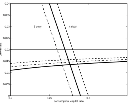
Considering next the case of a baby bust (η falls from 0.03 to 0.02), differentiation of (27) with respect to η yields:

∂ r ˆ

∂η = − ^{∂ γ ˆ}

∂η = − ^{∂ Φ r ˆ}

^{, η, β, α} /∂η

∂ Φ r ˆ

, η, β, α /∂ˆ r

> 0, (29)

d x ˆ

dη = − ^{∂ Γ} ( x, ˆ η, β, α ) /∂η

∂ Γ ( x, ˆ η, β, α ) /∂ x ˆ < 0,

where the signs in (29) follow from ˆ r

> ρ and ˆ r

> n − ( 1 − ε ) Z

. According to (29), a decline in fertility, since it reduces the importance of intergenerational turnover, leads to an increase in economic growth and rise in the consumption-capital ratio. Graphically, this shock is illustrated in Figure 2, where the post-shock Euler and the market clearing relationships (dashed) result in a new equilibrium with higher values of ˆ γ and ˆ x.

Finally, turning to the case of a longevity boom (β down from 0.02 to 0.01), we find:

∂ r ˆ

∂β = − ^{∂ γ ˆ}

∂β = − ^{∂ Φ r ˆ}

^{, η, β, α} /∂η

∂ Φ r ˆ

, η, β, α /∂ˆ r

> _{0, (30)}

d x ˆ

dβ = − ^{∂ Γ} ( x, ˆ η, β, α ) /∂β

∂ Γ ( x, ˆ η, β, α ) /∂ x ˆ > 0,

that this leads to a higher growth rate and — in contrast to a baby bust — a lower consumption- capital ratio. Because agents live longer, they have the incentive to accelerate the accumu- lation of capital, increasing the balanced growth rate ˆ γ. Since, however, this is spread-out over a longer lifetime, consumption falls relative to the stock of capital. We also illustrate this in Figure 2, which depicts the shift-up in EE

and the shift-down in CA (dash-dotted) that leads to an increase in ˆ γ and a fall in ˆ x.

10The sign of∂ˆr_g/∂βfollows from that of∂Φ/∂β, which equals ˆr_g−ρ−η/(1−α) <0. Since we can show ˆ

rg<ρ+η(see Appendix B), the latter holds whether or not 0<α<1 orα<0.

10

0.2 0.25 0.3 0

0.005 0.01 0.015 0.02 0.025 0.03 0.035 0.04

η down β down

consumption−capital ratio

growth rate

Figure 2: Growth and demographic shocks

6 Introducing a PAYG Pension System

We now extend the basic growth model to incorporate a PAYG pension system. Letting

¯

z ( v, τ ) denote taxes (and transfers if negative), contributions are paid and benefits are re- ceived according the following scheme:

z ¯ ( v, τ ) =

( θ · _w ( τ ) for τ − _v ≤ _u

− π · w ( τ ) for τ − v > u

, (31)

where θ is the contribution rate, π is the benefit rate (both indexed to the wage w ( τ ) ), and u

is the statutory retirement age. For realism, we assume that workers earn more than pensioners so that 1 − θ > π. As in the benchmark specification, labor supply is exogenous, although modified to reflect mandatory retirement:

n ¯ ( v, τ ) =

( 1 for τ − _v ≤ _u

0 for τ − v > u

. (32)

According to (32), agents supply a “full” unit of labor until retirement after which they cease to work. This permits us to define the macroeconomic participation rate as:

N ( t ) L ( t ) ≡

Z _t

−∞

n ¯ ( v, t ) l ( v, t ) dv =

Z _t

t−u_R

l ( v, t ) dv = 1 − e

, (33)

11

where N ( t ) is the work force. Clearly, the participation rate rises with u

, while a “baby bust” (decline in η) reduces it. This formulation allows us to define the dependency ratio as:

dr ≡ _dr ( u

, η ) = ^e

−ηuR

1 − e

, ∂dr

∂u

< _0, ^∂dr

∂η < _{0. (34)}

Not only does the PAYG system place a “wedge” between the workforce and the population, it also implies that an agent’s human wealth is age-dependent. Letting ¯ h ( v, τ ) represent individual human wealth, its weighted average equals:

h ( t ) ≡

Z _t

−∞

l ( v, t ) h ^¯ ( v, t ) dv. (35) Next, we impose sustainability of the PAYG system by assuming that contributions always equal payouts at all points in time:

Z _t

t−u_R

θw ( t ) L ( v, t ) dv =

Z _t−uR

−∞

πw ( t ) L ( v, t ) dv. (36) Substituting for L ( v, t ) = L ( t ) · _l ( v, τ ) , using (12), the closure rule reduces to:

θ · 1 − e

= π · e

, (37)

where one of θ, u

, and π must be used to balance the PAYG budget. Observe that under a defined benefit (DB) scheme, π and u

are held constant while θ balances the budget. In con- trast, θ and u

are held constant while π balances the budget under a defined contribution (DC) scheme. It is straightforward to show that the following relationships hold:

1 − θ − π =



 



 



1 − ^π

1 − e

DB 1 − _θe

_DC

. (38)

It follows that:

∂ ( 1 − _θ − _π )

∂u

> 0 (for DB), ∂ ( 1 − _θ − _π )

∂u

< 0 (for DC). (39)

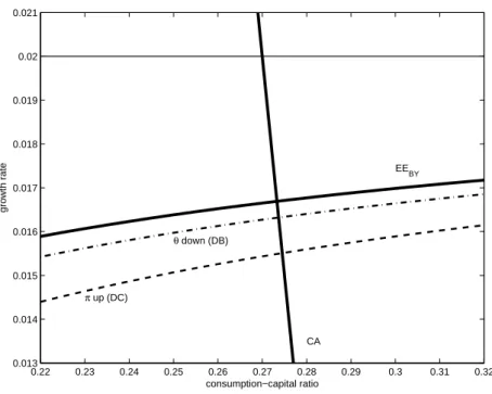
These results are important to investigate how a change in the statutory retirement date affects the balanced growth rate.

To solve the modified model, we follow the same procedure outlined above. The firm’s problem is solved as in section 2.1, with L

( t ) replaced by N

( t ) in (1), and with K ( t ) /N ( t ) affecting general productivity in (3). Since labor supply, according to (33), depends on the retirement date u

, so does the wage rate w ( t ) :

w ( t ) = ( 1 − ε ) ^Y ( t )

N ( t ) = ( 1 − ε ) ^Z

^k ( t )

1 − e

, (40)

12

where we substitute for Y ( t ) = Z

K ( t ) , N ( t ) ≡ [ 1 − e

] L ( t ) and use k ( t ) ≡ K ( t ) /L ( t ) to obtain (40). Observe that for a given value of k ( t ) , a later retirement date lowers the wage rate due to the expansion in labor supply.

Regarding the household’s problem, we proceed along the same lines as above, with the exception that the agent’s choices are made subject to (31). Consequently, we replace (7) by:

˙¯

a ( v, τ ) = [ r ( τ ) + β ] a ¯ ( v, τ ) + w ( τ ) − c ¯ ( v, τ ) − z ¯ ( v, τ ) . (41) Similarly, we replace h ( t ) with ¯ h ( v, t ) in the expression (11) for individual consumption. In turn, an active agent possesses a human wealth level of:

h ¯ ( v, t ) ≡

Z _v+uR

t

w ( τ ) e

dτ −

Z ∞

t

z ¯ ( v, τ ) e

dτ (42)

=

Z _v+uR

t

( 1 − _θ ) w ( τ ) e

dτ +

Z ∞ v+uR

πw ( τ ) e

dτ,

where we use (31) to obtain the second equality of (42). Substituting the path of wages in (42), w ( τ ) = w ( t ) · e

, τ ≥ t (with ˆ γ determined in equilibrium), a worker’s human wealth simplifies to:

h ¯ ( v, t ) = ^w ( t )

r

+ β · ^h ( 1 − _θ ) · ^h ₁ − _e (

)

i

+ π · _e (

)

i

, t − _v ≤ _u

_{. (43)} Correspondingly, a retired person’s human wealth is given by:

h ¯ ( v, t ) = π

t

w ( τ ) e

dτ = ^πw ( t ) ˆ

r

+ β , t − v > u

. (44)

To determine the economy’s Euler equation, we use the method described in Appendix A for the standard formulation. It is straightforward to show that (16) becomes:

˙ c ( t )

c ( t ) = r ( t ) − ρ − ^η ( ρ + β ) 1 − α ·

k ( t )

c ( t ) − ^{h ¯} ( t, t ) − h ( t ) c ( t )

, (45)

where consumption dynamics now also depends on the intergenerational turnover, [ h ^¯ ( t, t ) − h ( t )] , in human wealth. We show in Appendix C that [ h ^¯ ( t, t ) − h ( t )] equals:

h ¯ ( t, t ) − h ( t ) = w ( t ) e

( 1 − θ − π ) · ^e

−nu_R

− e

ˆ

r

− n > 0, (46)

where 1 − θ > π.

Clearly, agents are born with more human wealth than average, since they can look forward to the relatively longest period of high earnings. Moreover, the PAYG

11In the absence of a pension system,θ=π=0 andu_R →∞individual human wealth reduces to ¯h(v,t) = h(t) =w(t)/ rg+β

.

12Two further things are worth noting. First, the sign of (46) is guaranteed because ^e−nuR_ˆrg⁻_−n^{e−ˆrg uR} is positive regardlessof the sign of ˆrg−n. Second, under theAaron condition, ˆrg >n, it follows that for a given retirement ageu_R, a newborn has a lower level of human wealth under the PAYG system than in the absence of such a system (see Appendix D).

13

system affects the macroeconomy through the turnover in human wealth. Indeed, because newborn agents possess more human wealth than their older counterparts, this mitigates the fact that newborns are “asset poor” financially compared to older agents. This lessens the effects of intergenerational turnover in (45) and increases the growth in average consumption compared to an economy without a PAYG scheme, a result we prove subsequently. To sum- up, PAYG macroeconomic equilibrium consists of (45), where [ h ^¯ ( t, t ) − h ( t )] is given by (46).

The expressions for the interest rate are the same as stated in (18)–(19), while we replace the expression for the wage with (40). Finally, regarding market clearing, we replace (17) with:

k ˙ ( t ) = [ r − n ] k ( t ) + w ( t ) 1 − e

− c ( t ) . (47)

7 Pension Policy and Economic Growth

To investigate the implications of pension policy for economic growth, we first derive the modified economic dynamics. For the Euler relationship we substitute the equation for the wage w ( t ) from (40) in that of [ h ^¯ ( t, t ) − _h ( t )] from (46) and use y ( t ) = Z

k ( t ) . We then substitute the resulting expression in (45) to calculate:

˙ c ( t )

c ( t ) = r − _ρ − _σ Ω r ˆ

· ^k ( t )

c ( t ) ^{, (48)}

where ˆ r

≡ r − γ, ˆ σ ≡ η ( ρ + β ) / ( 1 − α ) is a positive constant, and:

Ω ( r ˆ

) ≡ 1 − ( 1 − ε ) r

ε · dr ( u

) · ( 1 − θ − π ) · ¹ − e

(

)

ˆ

r

− n > 0.

Observe that the difference between (48) and the Euler equation of the basic model (16) is that per capita consumption growth now depends on Ω ( r ˆ

) , which is itself a function of ˆ γ and incorporates features of the pension system. Similarly, combining (47) with (40) and y ( t ) = Z

k ( t ) , the market clearing condition simplifies to:

k ˙ ( t ) = [ r + ( 1 − _ε ) Z

− _n ] k ( t ) − _c ( t ) . (49) Evaluating (48)–(49) along the steady-state growth path ˆ γ and, as before, letting ˆ x ≡ c/ˆ ˆ k, we obtain:

ˆ

γ = r − ρ − σ Ω ( r − γ ˆ ) · ¹ ˆ

x , γ ˆ = r + ( 1 − ε ) Z

− x ˆ − n. (50) Observe that the expression for market clearing is identical to that from the basic model, implying that PAYG pensions affect the growth path only through the Euler relationship. To

13See Appendix C for the derivation of (47).

14

distinguish the framework with public pensions from that of the basic framework, we let ˆ r

(≡ r − γ ˆ

) and ˆ x

represent, respectively, the growth-adjusted interest rate and consumption- capital ratio under the PAYG plan. The system (50) becomes:

( r ˆ

− _ρ ) · x ˆ

= σ Ω ( r ˆ

) , x ˆ

= r ˆ

+ ( 1 − _ε ) Z

− _{n (51)} Combining the expressions in (51), we obtain the polynomial determining ˆ r

:

Φ ( r ˆ

, π, θ, u

) ≡ r ˆ

− _ρ · ^h r ˆ

+ ( 1 − _ε ) Z

− _n ⁱ − _σ Ω ( r ˆ

) ≡ _{0, (52)} where we indicate in (52) that the solution depends on the parameters of the PAYG system.

Equally, the polynomial solving for ˆ x

corresponds to:

Γ ˆ

x

, π, θ, u

= ( x ˆ

)

− [ ρ + ( 1 − ε ) Z

− n ] x ˆ

− σ Ω ( r ˆ

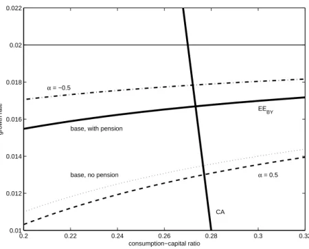
) ≡ 0. (53) We next show that the economy with PAYG pensions has a higher growth rate and a lower consumption-capital ratio than the economy lacking them. To do so, we linearize the polynomial Φ ( s ) given in (24) from the basic model about the PAYG equilibrium determined in (52). This yields:

( r ˆ

− ρ ) · [ r ˆ

+ ( 1 − ε ) Z

− n ] − σ + [ 2ˆ r

− ( ρ + n ) + ( 1 − ε ) Z

] · ( r ˆ

− r ˆ

) = 0. (54) Evaluating the first term in (54) at the PAYG equilibrium using (52), we solve for ( r ˆ

− r ˆ

) = ( γ ˆ

− γ ˆ ) :

ˆ

r

− r ˆ

= γ ˆ

− γ ˆ = ^σ [ 1 − Ω ( r ˆ

)]

2ˆ r

− ( ρ + n ) + ( 1 − ε ) Z

> 0, (55)

which implies that the balanced rate of growth is higher if agents receive PAYG pensions.

The reason for our finding is that the PAYG system imposes a life-cycle on human wealth that does not otherwise obtain in the standard BY framework. In our specification the PAYG pension puts part of the population, since ( 1 − θ ) > π, in a lower non-asset income stream.

This strengthens the effect of the turnover in human wealth, [ h ^¯ ( t, t ) − _h ( t )] > 0, since agents are now born with relatively more human wealth than their older counterparts who face re- duced non-asset retirement income. This, in turn, weakens the negative implications that demographic turnover has, in general, on economic growth. Under consumption smooth- ing, agents respond to the fall in old-age income by increasing saving during their working

14The sign of (55) is positive since:

1−^Ω(rˆg) = (1−ε)r

ε dr(π_R) (1−θ−π)¹−e^{−(ˆrg−n)uR} ˆ

rg−n >0.

15

0.2 0.22 0.24 0.26 0.28 0.3 0.32 0.01

0.012 0.014 0.016 0.018 0.02 0.022

α = 0.5 base, with pension

base, no pension α = −0.5

CA

EEBY

consumption−capital ratio

growth rate

Figure 3: Growth, pensions, and the KUJ effect

lives, which raises the rate of capital accumulation and implies that ˆ γ

> γ. In turn, the ˆ expression for ˆ x − x ˆ

, obtained by linearizing Γ ( s ) from (25) about the equilibrium solved for in (53), equals:

ˆ

x

− x ˆ = − ¹ − ^Ω ( r ˆ

)

2ˆ r

− ( ρ + n ) + ( 1 − ε ) Z

< 0, (56)

We depict in Figure 3 the influence of PAYG, where the baseline pension system parame- ters equal:

dr = 0.20, u

= 59.73 years, θ = 0.1, π = 0.5, rr ≡ ^π

1 − _θ = 0.45. (57) The growth equilibrium with pensions is illustrated by the intersection of the solid EE

and CA relationships: since the solid EE

locus lies entirely above its counterpart in Figure 1 with no pensions (the thinly dotted line), the solution ( x, ˆ ˆ γ ) under PAYG involves a higher growth rate and a lower consumption-capital ratio. Figure 3 furthermore illustrates how KUJ modifies the role of the pension system. Admiration (α = − 0.5) augments the effect of PAYG, raising the growth rate even more, while jealousy (α = 0.5) reverses it. Indeed, under our parameterization, jealousy is more ‘powerful’ than PAYG, since ˆ γ

< γ ˆ

, a result depicted in Figure 3 by comparing the dotted and dashed relationships.

16