SFB 823
Testing monotonicity of Testing monotonicity of Testing monotonicity of Testing monotonicity of regression functions
regression functions regression functions
regression functions – – – – an an an an empirical process approach empirical process approach empirical process approach empirical process approach
D is c u s s io n P a p e r
Melanie Birke, Natalie Neumeyer
Nr. 9/2010
Testing monotonicity of regression functions – an empirical process approach
Melanie Birke
Ruhr-Universit¨at Bochum Fakult¨at f¨ur Mathematik
Universit¨atsstraße 150 44780 Bochum, Germany
e-mail: melanie.birke@ruhr-uni-bochum.de
Natalie Neumeyer Universit¨at Hamburg Department Mathematik
Bundesstraße 55 20146 Hamburg, Germany
e-mail: neumeyer@math.uni-hamburg.de
April 6, 2010
Abstract
We propose several new tests for monotonicity of regression functions based on different empirical processes of residuals. The residuals are obtained from recently developed simple kernel based estimators for increasing regression functions based on increasing rearrangements of unconstrained nonparametric estimators. The test statis- tics are estimated distance measures between the regression function and its increasing rearrangement. We discuss the asymptotic distributions, consistency, and small sample performances of the tests.
AMS Classification: 62G10, 62G08, 62G30
Keywords and Phrases: Kolmogorov-Smirnov test, model test, monotone rearrangements, nonparametric regression, residual processes
1 Introduction
In a nonparametric regression context with regression functionm we consider the important problem of testing for monotonicity of the regression function, i. e. testing for validity of the null hypothesis
H0 : “m is increasing”.
First literature on testing for monotonicity of regression function is given by Schlee (1982) who proposes a test which is based on estimates of the derivative of the regression func- tion. Bowman, Jones and Gijbels (1998) used Silverman’s (1981) “critical bandwidth” ap- proach to construct a bootstrap test for monotonicity, while Gijbels, Hall, Jones and Koch (2000) considered the length or runs of consecutive negative values of observation differ- ences. Hall and Heckman (2000) suggested to fit straight lines through subsequent groups of consecutive points and reject monotonicity for too large negative values of the slopes.
Other recent work on testing monotonicity can be found in Goshal, Sen and Van der Vaart (2000), D¨umbgen (2002), Durot (2003), Baraud, Huet and Laurent (2003) and Dom´ınguez- Menchero, Gonz´alez-Rodr´ıguez and L´opez-Palomo (2005). Birke and Dette (2007) consider a test for strict monotonicity based on the L2-distance of the distribution function of the unconstrained estimator evaluated at the unconstrained estimator to the identity (see sec- tion 3 for more comments on that test). Most tests for monotonicity suffer from the problem of underestimating the level because they are calibrated with the most difficult null model which is a constant regression function. Gijbels (2005) gives a thorough review on tests for monotonicity of regression functions and suggests as alternative “to base a test statistic on a measure of the distance between an unconstrained and a constrained estimate of the regression function”. However, to the authors’ best knowlegde in the paper at hand for the first time those tests for monotonicity are investigated. For similar testing problems (for in- stance, testing whethermbelongs to a parametric class of functions) such tests based on an estimated norm difference between an estimator under H0 and an unconstrained estimator are very popular. In our context, such tests would be based, for example, on an estimated L2-distance between a completely nonparametric regression estimator ˆm and an increasing estimator ˆmI constructed under the null hypothesis; see H¨ardle and Mammen (1993) for such a test in the goodness-of-fit context. Other test statistics could be constructed sim- ilar to the goodness-of-fit tests by Stute (1997) or Van Keilegom, Gonz´alez-Manteiga and S´anchez Sellero (2008) based on estimated empirical processes of residuals (see section 3 for exact definitions of those processes). To do so one needs an estimator for the regression function under the null hypothesisH0 of monotonicity. Such increasing regression estimators were proposed by Mammen (1991), Hall and Huang (2001), and Dette, Neumeyer and Pilz (2006), among others. The mentioned methods have in common that they are based on a preliminary unconstrained estimator ˆm and are (under appropriate assumptions) first order asymptotically equivalent to each other and to the unconstrained estimator ˆm. This is a nice and desirable property for estimation purposes, but it limits the application of such estimators for testing monotonicity by distance based tests as suggested before. It turns out that those typical distance based test that are so popular in testing for different model assumptions have, when testing for monotonicity, degenerate limit distributions under the
null hypothesis and, hence, are not suitable for testing.
The intuitive idea we follow in the present paper instead is as follows. We investigate the behaviour of pseudo-residuals built under the hypothesisH0 of monotonicity, which estimate pseudo-errors that coincide with the true errors in general only under the null hypothesis.
Whereas the true errors are assumed to be independent and identically distributed, the pseudo-errors behave differently. We construct several test statistics to detect these different behaviours. The test statistics are based on several empirical processes of (pseudo-)residuals.
To build the pseudo-residuals, we estimate the regression function underH0 by applying the simple kernel based increasing estimator by Dette, Neumeyer and Pilz (2006) [see also Birke and Dette (2008) for further discussion of this estimator]. Under the null hypothesis we show weak convergence of the empirical processes to Gaussian processes. The asymptotic distributions are independent of the regression function m and, hence, the tests need not be calibrated using a most difficult null model. For normal regression models we can even obtain asymptotically distribution free tests. The test statistics turn out to be estimators for certain distance measures between the true regression function m and an “increasing version” mI of m, and hence, are consistent. Moreover, the tests can detect local alterna- tives of convergence rate n−1/2. To the authors’ best knowledge those are the first tests in literature for testing monotonicity of regression functions with this property. We compare the small sample behavior of the empirical process approaches to that of theL2-test in Birke and Dette (2007) and observe, that they are less conservative and can in fact better detect local alternatives of convergence rate n−1/2.
The paper is organized as follows. In section 2 we define the monotone regression estima- tor and list the model assumptions. Section 3 motivates and defines the test statistics, for which the asymptotic distributions are stated in section 4. In section 5 we explain bootstrap versions of the tests and investigate the small sample behaviour, whereas some concluding remarks are given in section 6. All proofs are given in an appendix.
2 Model and assumptions
Consider the nonparametric regression model
Yi = m(Xi) +εi, i= 1, . . . , n,
where (Xi, Yi), i= 1, . . . , n, is a bivariate sample of i.i.d. observations. If there is evidence that the regression function m is increasing we define
ˆ
m−I1(t) = 1 bn
Z 1
0
Z t
−∞
km(v)ˆ −u bn
dudv
as an estimate ofm−1(t),where ˆm denotes a local linear estimator form with kernel K and bandwidth hn. [By increasing throughout the paper we mean nondecreasing in distinction from strictly increasing.]
The estimator ˆmI is defined as the generalized inverse of ˆm−I1, that is ˆ
mI(x) = inf{t ∈IR|mˆ−I1(t)≥x}.
Under H0 and under the following assumptions ˆmI is asymptotically first order equivalent to the unconstrained estimator ˆm, see Dette, Neumeyer and Pilz (2006). This is a smoothed version of the monotone rearrangement (see e.g. Hardy, Littlewood and Poly´a, 1952 or Lieb and Loss, 2001)
(A1) The covariates X1, . . . , Xn are independent and identically distributed with distribu- tion function FX on compact support, say [0,1]. FX has a twice continuously differ- entiable density fX such that infx∈[0,1]fX(x) > 0. The regression function m is twice continuously differentiable.
(A2) K and k are symmetric, twice continuously differentiable kernels of order 2 with bounded supports, say (−1,1), such that K(−1) =K(1) =k(−1) =k(1) = 0.
(A3) The bandwidths fulfill hn, bn →0,nhn, nbn→ ∞ and nh4n→0, nb4n →0, b2nlog(h−n1)
hn →0, log(h−n1)
nh3nb4δn →0, log(h−n1) nhnb2n →0 for some δ ∈(0,12) and for n→ ∞.
(A4) The errorsε1, . . . , εnare independent and identically distributed, independent from the covariates, with strictly increasing distribution function Fε and bounded density fε, which has one bounded continuous derivative. The errors are centered, i. e. E[εi] = 0 with variance σ2 >0 and existing fourth moment.
(A5) The errors have median zero, i. e. Fε(0) = 12.
(A6) The errors ε1, . . . , εn are independent and normally distributed with expectation zero and variance σ2 >0, independent from the covariates.
(A7) The error density fε is unimodal.
Conditions (A1)–(A4) are assumed to be valid throughout the paper, whereas it is stated explicitly when (A5), (A6) or (A7) are assumed.
We restrict to the homoscedastic case with random covariates for the moment, but other cases will be discussed in Remarks 4.4 and 4.5.
3 Test statistics
In general the estimator ˆmI estimates the increasing rearrangement mI of m. Only under the hypothesisH0 of an increasing regression function we have m=mI. We build (pseudo-) residuals
ˆ
εi,I =Yi−mˆI(Xi),
which estimate pseudo-errors εi,I = Yi −mI(Xi) that coincide with the true errors εi = Yi−m(Xi) (i= 1, . . . , n) in general only under H0. Let further
ˆ
εi =Yi−m(Xˆ i)
denote the unconstrained residuals. Under H0 both ˆm and ˆmI join the same first order asymptotic expansion. This for estimation purposes very desirable property limits the possi- bilities to apply the estimator ˆmI for hypotheses testing. Test statistics based on estimated empirical processes such as
√1 n
n
X
i=1
ˆ
εi,II{Xi ≤ ·} or 1
√n
n
X
i=1
I{εˆi,I ≤ ·} −I{εˆi ≤ ·}
(3.1)
[compare to Stute (1997) and Van Keilegom, Gonz´alez-Manteiga and S´anchez Sellero (2008)]
are of convergence orderoP(1) and not suitable for the testing problem considered here. For the estimated L2-distance
nh1/2n Z
( ˆmI −m)ˆ 2 (3.2)
[cf. H¨ardle and Mammen (1993)] the same problem arises. One could try to rescale the test statistics and apply second order asymptotic expansions to derive an nondegenerate limit distribution. Whereas this seems not possible for the second empirical process in (3.1) with methods of proofs typically applied for such processes, it might work for the first process in (3.1) as well as for the L2-distance test (3.2). However, the resulting tests typically react rather sensitive to the choice of smoothing parameters. Birke and Dette (2007) follow this approach by considering a suitably scaled version of the test statisticR
( ˆm−I1( ˆm(x))−x)2dx and by applying second order asymptotic expansions.
The idea we follow in the present paper instead is the following. Whereas the true er- rors ε1, . . . , εn are assumed to be independent and identically distributed, the pseudo-errors ε1,I, . . . , εn,I behave differently. If the true function m is not monotone (e.g. like in Figure 1) and we calculate the pseudo-residuals frommI too many of them are positive (see solid dots with black lines) on some subinterval of [0,1] and too many are negative (see open dots with grey lines) on another subinterval. Therefore, they are no longer identically distributed if H0 is not fulfilled.
0 1 0
1
m mI
0 t0 1
0 1
m mI
Figure 1: Left part: True function m (grey line), monotonized function mI (black line) together with observations. Right part: Pseudo-residuals (positive ones solid with black dashed lines, negative ones open with grey dashed lines)
We construct test statistics from several estimated empirical processes to detect this different behaviour. The first process we will consider is defined as
Sn(t) = 1
√n
n
X
i=1
I{εˆi,I >0}I{Xi ≤t} − 1
2FˆX,n(t)
where t ∈ [0,1] and ˆFX,n denotes the empirical distribution function of the covariates X1, . . . , Xn. For every t ∈ [0,1] it counts how many pseudo-residuals are positive up to covariates ≤t. This term is then centered with respect to the estimated expectation under H0 and scaled with n−1/2. Under assumptions (A1)–(A5), Sn(t) consistently estimates the expectation
√n
E[I{εi,I >0}I{Xi ≤t}]− 1
2FX(t)
= √ n
E[I{εi >(mI −m)(Xi)}I{Xi ≤t}]−(1−Fε(0))FX(t) (3.3)
= √ n
Z t
0
Fε(0)−Fε((mI −m)(x))
fX(x)dx.
This term is zero for all t ∈ [0,1] if and only if mI = m is valid FX-a. s. To obtain this equivalence one especially uses that Fε is strictly increasing, whereas equality (3.3) applies assumption (A5). As we have seen, for instance a Kolmogorov-Smirnov type statistic sn = supt∈[0,1]|Sn(t)| estimates a distance measure between mI and m and, to obtain a consistent testing procedure, the null hypothesis should be rejected for large values ofsn.
To avoid assumption (A5) one can alternatively consider the process S˜n(t) = √
n1 n
n
X
i=1
I{εˆi,I >0}I{Xi ≤t} −(1−Fˆε,n(0)) ˆFX,n(t) ,
where ˆFε,n denotes the empirical distribution function of ˆε1, . . . ,εˆn.
The application of tests based on Sn and ˜Sn may not lead to good power in cases where m and mI are quite similar and the variance is large. Hence it seems sensible to not only take into account the sign of the estimated pseudo-errors, but also their value, i. e. to consider tests based on
1 n
n
X
i=1
ˆ
εi,II{εˆi,I >0}I{Xi ≤t}.
The estimated expectation of this term under H0, i. e. E[εiI{εi > 0}I{Xi ≤ t}] is known to be √σ2πFX(t) under assumption (A6), and then can be estimated by √σˆ2πFˆX,n(t), where ˆ
σ= (n−1Pn
i=1εˆ2i)1/2. This leads to the process Vn(t) = √
n1 n
n
X
i=1
ˆ
εi,II{εˆi,I >0}I{Xi ≤t} − σˆ
√2π
FˆX,n(t) . To avoid assumption (A6) one can alternatively consider the process
V˜n(t) = √ n1
n
n
X
i=1
ˆ
εi,II{εˆi,I >0}I{Xi ≤t} − 1 n
n
X
i=1
ˆ
εiI{εˆi >0}FˆX,n(t) .
Lemma 3.1 Tests that for some constant c > 0 reject H0 whenever supt∈[0,1]|Vn(t)| > c or supt∈[0,1]|V˜n(t)| > c are consistent under assumptions (A1)–(A3),(A6) and (A1)–(A4), respectively.
Because the proof of this statement requires a longer argumentation we defer it to the appendix.
Now let ˆRi,I denote the fractional rank of ˆεi,I with respect to ˆε1,I, . . . ,εˆn,I, i. e.
Rˆi,I = 1 n
n
X
j=1
I{εˆj,I ≤εˆi,I} and consider the term
1 n
n
X
i=1
Rˆi,II{εˆi,I >0}I{Xi ≤t}, which (underH0) estimates the expectation
Eh1 n
n
X
j=1
I{εj ≤εi}I{εi >0}I{Xi ≤t}i
= E[Fε(εi)I{εi >0}]FX(t) +o(1)
= Z 1
Fε(0)
x dx FX(t) +o(1) = 1
2 − (Fε(0))2 2
FX(t) +o(1) = 3
8FX(t) +o(1),
where the last equality holds under assumption (A5). This expectation can be estimated by
3
8FˆX,n(t) under (A5) and by 12(1−( ˆFε,n(0))2) ˆFX,n(t) otherwise, which leads to the empirical processes
Rn(t) = 1
√n
n
X
i=1
Rˆi,II{εˆi,I >0}I{Xi ≤t} − 3
8FˆX,n(t) R˜n(t) = 1
√n
n
X
i=1
Rˆi,II{εˆi,I >0}I{Xi ≤t} − 1
2(1−( ˆFε,n(0))2) ˆFX,n(t) .
Lemma 3.2 Tests that for some constant c > 0 reject H0 whenever supt∈[0,1]|Rn(t)|> c or supt∈[0,1]|R˜n(t)|> care consistent under assumptions (A1)–(A5),(A7) and (A1)–(A4),(A7), respectively.
Again, the proof of this result needs a longer argumentation and is defered to the appendix.
4 Main asymptotic results
In the following theorem we state weak convergence results for the processes defined before.
Note that we have to assume a strictly increasing regression function to derive the asymptotic distributions. Nevertheless, the monotone regression estimator ˆmI can also be applied for monotone regression functions with flat parts, see Dette and Pilz (2006).
Theorem 4.1 Assume that m′ is positive in [0,1].
(i)Under assumptions (A1)–(A5) the processSnconverges weakly inℓ∞([0,1])to a Gaussian process S with covariance
Cov(S(s), S(t)) = FX(s∧t)1
4+σ2fε2(0) + 2fε(0)E[ε1I{ε1 ≤0}]
= FX(s∧t)(1 4− 1
2π),
where the last equality holds under the additional assumption (A6).
(ii) Under assumptions (A1)–(A4) the process S˜n converges weakly in ℓ∞([0,1]) to a Gaus- sian process S˜ with covariance
Cov( ˜S(s),S(t))˜
= (FX(s∧t)−FX(s)FX(t))
Fε(0)(1−Fε(0)) +σ2fε2(0) + 2fε(0)E[ε1I{ε1 ≤0}]
= (FX(s∧t)−FX(s)FX(t))(1 4 − 1
2π),
where the last equality holds under the additional assumption (A6).
(iii) Under assumptions (A1)–(A3) and (A6) the process Vn converges weakly in ℓ∞([0,1])
to a Gaussian process V with covariance
Cov(V(s), V(t)) = FX(s∧t)(1 4 − 1
2π)σ2−FX(s)FX(t)σ2 4π.
(iv)Under assumptions (A1)–(A4) the process V˜n converges weakly in ℓ∞([0,1]) to a Gaus- sian process V˜ with covariance
Cov( ˜V(s),V˜(t))
= (FX(s∧t)−FX(s)FX(t))
(2Fε(0)−1)E[ε21I{ε1 ≤0}]−(E[ε1I{ε1 ≤0}])2+σ2(1−Fε(0))2
= (FX(s∧t)−FX(s)FX(t))(1 4 − 1
2π)σ2,
where the last equality holds under the additional assumption (A6).
(v) Under assumptions (A1)–(A5) the process Rn converges weakly in ℓ∞([0,1]) to a Gaus- sian process R with covariance
Cov(R(s), R(t))
= (FX(s∧t)−FX(s)FX(t)) 29
192 +σ2(fε(0)Fε(0)−E[fε(ε1)I{ε1 >0}])2 + 2E[Fε(ε1)ε1I{ε1 ≤0}](fε(0)Fε(0)−E[fε(ε1)I{ε1 >0}])
+ 1
16FX(s)FX(t).
(vi)Under assumptions (A1)–(A4) the process R˜n converges weakly inℓ∞([0,1]) to a Gaus- sian process R˜ with covariance
Cov( ˜R(s),R(t))˜
= (FX(s∧t)−FX(s)FX(t))
E[Fε2(ε1)I{ε1 >0}]−(E[Fε(ε1)I{ε1 >0}])2 +σ2(fε(0)Fε(0) +E[fε(ε1)I{ε1 >0}])2
−2E[Fε(ε1)ε1I{ε1 ≤0}](fε(0)Fε(0) +E[fε(ε1)I{ε1 >0}]) . The proof is given in the appendix.
Remark 4.2 For a normal regression model, i. e. under assumption (A6) we can obtain asymptotically distribution free tests, because then
sup
t∈[0,1]|Sn(t)|= sup
s∈(0,1)|Sn(FX−1(s))|
converges in distribution to (14 − 2π1 ) sups∈[0,1]|W(s)| for a Brownian motion W. Similarly, supt∈[0,1]|S˜n(t)| converges in distribution to (14−2π1 ) sups∈[0,1]|B(s)|, where B is a Brownian bridge.
Remark 4.3 The proposed tests can detect local alternatives of the form H1,n :m(x) =mI(x) + ∆(x)
√n ,
where ∆ 6= 0 on an interval in [0,1] of positive length. Consider Sn for simplicity. From (3.3) we see that the asymptotic expectation ofSn(t) under H1,n is
√n Z t
0
Fε(0)−Fε((mI −m)(x))
fX(x)dx=fε(0) Z t
0
∆(x)fX(x)dx+o(1).
With similar arguments as in the proof of Theorem 4.1 one can show that under H1,n, Sn converges in distribution to the process fε(0)Rt
0∆(x)fX(x)dx +S(t), t ∈ [0,1]. The Kolmogorov-Smirnov test statistic supt∈[0,1]|Sn(t)| constructed from Theorem 4.1 detects H1,n because fε(0) supt∈[0,1]|Rt
0 ∆(x)fX(x)dx|>0.
Remark 4.4 Assume a heteroscedastic regression model
Yi = m(Xi) +σ(Xi)εi, i= 1, . . . , n,
where Xi and εi are independent, E[ε2i] = 1, E[ε4i] < ∞, the regression function m, error distributionFε and covariate distributionFX fulfill assumptions as before, whereas the vari- ance function σ2 is twice continuously differentiable and bounded away from zero. Then similar tests for monotonicity of the regression function m can be constructed by replacing residuals ˆεi and pseudo-residuals ˆεi,I from before by
ˆ
εi = Yi−m(Xˆ i) ˆ
σ(Xi) , εˆi,I = Yi−mˆI(Xi) ˆ
σ(Xi) ,
where ˆσ2 denotes a Nadaraya-Watson estimator for σ2 with kernel K and bandwidth hn
based on “observations” (Yi−m(Xˆ i))2. With these changes the same processes as before can be considered for testingH0. Weak convergence to Gaussian processes can be obtained with methods as in Akritas and Van Keilegom (2001), where the asymptotic covariances change in comparison to Theorem 4.1 due to the estimation of the variance function.
Remark 4.5 Assume a (homoscedastic) fixed design regression model Yi = m(xni) +εi, i= 1, . . . , n,
with assumptions as before but with nonrandom covariatesxn1 ≤. . .≤xnn such that there exists a distribution functionFX with support [0,1] so that FX(xni) = ni, i = 1, . . . , n, and FX fulfills assumptions as before. Then similar tests for monotonicity of m can be derived by considering sequential empirical processes. For instance, instead of ˜Snwe would consider
S¯n(t) = √ n1
n
⌊nt⌋
X
i=1
I{εˆi,I >0} −(1−Fˆε,n(0))t ,
where ⌊nt⌋ is the largest integer ≤ nt. Weak convergence of the processes similar to the results in Theorem 4.1 can be obtained with methods as in Neumeyer and Van Keilegom (2009).
5 Bootstrap method and simulation results
Since the asymptotic distributions of the test statistics still depend on the unknown functions m and f we use the bootstrap procedures to construct tests based on the above statistics.
We build bootstrap observations that fulfill the null hypothesis by defining Yi∗ = ˆmI(Xi) +ε∗i, i= 1, . . . , n.
Here, under assumption (A6) we can generate the bootstrap errorsε∗1, . . . , ε∗n by the normal distributionN(0,σˆ2), where ˆσ2 is the estimated variance from residuals ˆε1, . . . ,εˆn.
Without assumption (A6) instead we apply a nonparametric smoothed residual bootstrap.
To this end, we randomly draw ˜ε∗i with replacement from centered residuals ˜ε1, . . . ,ε˜n, where
˜
εj = ˆεj−n−1Pn
k=1εˆk. Let further adenote a small smoothing parameter and let Z1, . . . , Zn
be independent and standard normally distributed. Then, ε∗i = ˜ε∗i +aZi, i = 1, . . . , n, are independent, given the original sampleYn={(Xi, Yi)|i= 1, . . . , n}and have a distribution function ˜Fn,ε with density
f˜n,ε(y) = 1 na
n
X
i=1
ϕε˜i−y a
.
From the bootstrap observations calculate the constrained and unconstrained regression estimators ˆm∗I and ˆm∗ and build residuals ˆεi,I = Yi∗ −mˆ∗I(Xi) and ˆε∗i = Yi∗ − m(Xˆ i), respectively. Let ˆFε,n∗ denote the empirical distribution function of ˆε∗1, . . . ,εˆ∗n and ˆR∗i,I the fractional rank of ˆε∗i,I with respect to ˆε∗1,I, . . . ,εˆ∗n,I. The bootstrap versions of the considered processes are defined as follows,
Sn∗(t) = √ n1
n
n
X
i=1
I{εˆ∗i,I >0}I{Xi ≤t} −(1−F˜ε,n(0)) ˆFX,n(t) S˜n∗(t) = √
n1 n
n
X
i=1
I{εˆ∗i,I >0}I{Xi ≤t} −(1−Fˆε,n∗ (0)) ˆFX,n(t) Vn∗(t) = √
n1 n
n
X
i=1
ˆ
ε∗i,II{εˆ∗i,I >0}I{Xi ≤t} − σˆ∗
√2πFˆX,n(t) V˜n∗(t) = √
n1 n
n
X
i=1
ˆ
ε∗i,II{εˆ∗i,I >0}I{Xi ≤t} − 1 n
n
X
i=1
ˆ
ε∗iI{εˆ∗i >0}FˆX,n(t) R∗n(t) = 1
√n
n
X
i=1
Rˆ∗i,II{εˆ∗i,I >0}I{Xi ≤t} − 1
2(1−( ˜Fε,n(0))2) ˆFX,n(t)
40 60 80 100
0.020.040.060.080.100.120.14
n
Size,σ=0.025
40 60 80 100
0.010.020.030.040.050.060.070.08
n
Size,σ=0.05
40 60 80 100
0.000.010.020.030.040.050.06
n
Size,σ=0.1
40 60 80 100
0.20.40.60.81.0
n
Power,σ=0.025
40 60 80 100
0.20.40.60.81.0
n
Power,σ=0.05
40 60 80 100
0.20.40.60.81.0
n
Power,σ=0.1
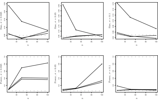
Figure 2: Simulated size and power in dependence of n for the tests ϕsn (diamonds), ϕvn (dots) and ϕrn (triangles) compared to the test ϕL2 (dashed line) for different standard deviations σ (left σ = 0.025, middle σ = 0.05, right σ = 0.1). First row m1, second row m2,n.
R˜∗n(t) = 1
√n
n
X
i=1
Rˆ∗i,II{εˆ∗i,I >0}I{Xi ≤t} − 1
2(1−( ˆFε,n∗ (0))2) ˆFX,n(t) ,
where only in the case ofVn∗under assumption (A6) we use the parametric bootstrap applying the normal distribution as explained above, where then ˆσ∗ is the empirical standard deviation of ˆε∗1, . . . ,εˆ∗n. Note that the bootstrap processes are centered in a slightly different way than the original statistics with the aim to obtain processes that are asymptotically centered with respect to the conditional expectation E[· | Yn]. In the appendix we sketch a proof for validity of the bootstrap procedures.
Since it turned out in a simulation study in Birke and Dette (2007), that their test and the test developed by Bowman, Jones and Gijbels (1998) behave very similar we will compare the tests described here only to the one by Birke and Dette (2007). More precisely we use the Kolmogorov-type statistics sn = sup|Sn(t)|, vn = sup|Vn(t)|, rn = sup|Rn(t)|,
˜
sn= sup|S˜n(t)|, ˜vn = sup|V˜n(t)|and ˜rn = sup|R˜n(t)|and denote the corresponding tests by ϕsn, ϕvn,ϕrn, ˜ϕsn, ˜ϕvn and ˜ϕrn. We show the behavior of all tests under the null hypothesis