UNIVERSITY OF DORTMUND
REIHE COMPUTATIONAL INTELLIGENCE COLLABORATIVE RESEARCH CENTER 531
Design and Management of Complex Technical Processes and Systems by means of Computational Intelligence Methods
Towards a Theory of Randomized Search Heuristics
Ingo Wegener
No. CI-169/04
Technical Report ISSN 1433-3325 February 2004
Secretary of the SFB 531 · University of Dortmund · Dept. of Computer Science/XI 44221 Dortmund·Germany
This work is a product of the Collaborative Research Center 531, “Computational Intelligence,” at the University of Dortmund and was printed with financial support of the Deutsche Forschungsgemeinschaft.
Towards a Theory of Randomized Search Heuristics
Ingo Wegener
FB Informatik, LS 2, Univ. Dortmund, 44221 Dortmund, Germany wegener@ls2.cs.uni-dortmund.de
Abstract. There is a well-developed theory about the algorithmic com- plexity of optimization problems. Complexity theory provides negative results which typically are based on assumptions like NP=P or NP=RP.
Positive results are obtained by the design and analysis of clever algo- rithms. These algorithms are well-tuned for their specific domain. Prac- titioners, however, prefer simple algorithms which are easy to implement and which can be used without many changes for different types of prob- lems. They report surprisingly good results when applying randomized search heuristics like randomized local search, tabu search, simulated an- nealing, and evolutionary algorithms. Here a framework for a theory of randomized search heuristics is presented. It is discussed how random- ized search heuristics can be delimited from other types of algorithms.
This leads to the theory of black-box optimization. Lower bounds in this scenario can be proved without any complexity-theoretical assump- tion. Moreover, methods how to analyze randomized search heuristics, in particular, randomized local search and evolutionary algorithms are presented.
1 Introduction
Theoretical computer science has developed powerful methods to estimate the algorithmic complexity of optimization problems. The borderline between poly- nomial-time solvable and NP-equivalent problems is marked out and this holds for problems and their various subproblems as well as for their approximation variants. We do not expect that randomized algorithms can pull down this bor- der.
The “best” algorithms for specific problems are those with the smallest asymptotic (w.r.t. the problem dimension) worst-case (w.r.t. the problem in- stance) run time. They are often well-tuned especially for this purpose. They can be complicated, difficult to implement, and not very efficient for reasonable problem dimension. This has led to the area of algorithm engineering.
Nevertheless, many practitioners like another class of algorithms, namely so- called randomized search heuristics. Their characteristics are that they are
This work was supported by the Deutsche Forschungsgemeinschaft (DFG) as part of the Collaborative Research Center “Computational Intelligence” (SFB 531), the Collaborative Research Center “Complexity Reduction of Multivariate Data Struc- tures” (SFB 475), and the GIF project “Robustness Aspects of Algorithms”.
– easy to implement, – easy to design,
– often fast although there is no guaranteed upper bound on the expected run time,
– often producing good results although there is no guarantee that the solution is optimal or close to optimal.
Classical algorithm theory is concerned with guarantees on the run time (or the expected run time for randomized algorithms) and with guarantees for the quality of the results produced by the algorithm. This has led to the situation that practitioners work with algorithms which are almost not considered in the theory of algorithms.
The motivation of this paper is the following. If randomized search heuristics find many applications, then there should be a theory of this class of algorithms.
The aim is to understand how these algorithms work, what they can achieve and what they cannot achieve. This should lead to the design of better heuristics, rules which algorithm is appropriate under certain restrictions, and an at least partial analysis of these algorithms on selected problems. Finally, these results can be used when teaching randomized search heuristics.
The problem is that we are interested in “the best” algorithms for an op- timization problem and we do not expect that a randomized search heuristic is such a best algorithm. It seems to be impossible to define precisely which algorithm is a randomized search heuristic. Our solution to this dilemma is to describe an algorithmic scenario such that all known randomized search heuris- tics can work in this scenario while most problem-specific algorithms are not applicable in this scenario. This black-box scenario is presented in Section 2.
There it is shown that black-box algorithms can be interpreted as randomized decision trees. This allows the application of methods from classical complexity theory, in particular, lower-bound methods like Yao’s minimax principle.
This new framework allows a general theory of black-box algorithms includ- ing randomized local search, tabu search, simulated annealing, and evolutionary algorithms. Theoretical results on each of these classes of randomized search heuristics were known before, e.g., Papadimitriou, Sch¨affer, and Yannakakis (1990) for local search, Glover and Laguna (1993) for tabu search, Kirkpatrick, Gelatt, and Vecchi (1983) and Sasaki and Hajek (1998) for simulated annealing, and Rabani, Rabinovich, and Sinclair (1998), Wegener (2001), Droste, Jansen, and Wegener (2002), and Giel and Wegener (2003) for evolutionary algorithms.
Lower bounds on the complexity of black-box optimization problems are pre- sented at the end of this paper, in Section 9. Before, we investigate what can be achieved by randomized search heuristics, in particular, by randomized local search and evolutionary algorithms. The aim is to present and to apply methods to analyze randomized search heuristics on selected problems. In Section 3, we, therefore, discuss some methods which have been applied recently and, after- wards, we present examples of these applications. In Section 4, we investigate the optimization of degree-bounded polynomials which are monotone with re- spect to each variable. It is not known whether the polynomial is increasing or
decreasing withxi.Afterwards, we investigate famous problems with well-known efficient algorithms working in the classical optimization scenario. In Section 5, we investigate sorting as the maximization of sortedness. The sortedness can be measured in different ways which has influence on the optimization time of evolutionary algorithms. In Section 6, the single-source-shortest-paths problem is discussed. It turns out that this problem can be handled efficiently only in the model of multi-objective optimization. In Section 7, the maximum matching problem is investigated in order to show that evolutionary algorithms can find improvements which are not obtainable by single local operations. Evolutionary algorithms work with two search operators known as mutation and crossover. In Section 8, we discuss the first analytic results about the effectiveness of crossover.
The results on the black-box complexity in Section 9 show that the considered heuristics are close to optimal — in some cases. We finish with some conclusions.
2 The Scenario of Black-Box Optimization
The aim is to describe an algorithmic scenario such that the well-known ran- domized search heuristics can work in this scenario while it is not possible to apply “other algorithms”. What are the specific properties of randomized search heuristics? The main observation is that randomized search heuristics use the information about the considered problem instance in a highly specialized way.
They do not work with the parameters of the instance. They only compute pos- sible solutions and work with the values of these solutions. Consider, e.g., the 2-opt algorithm for the TSP. It starts with a random tourπ. In general, it stores one tourπ, cuts it randomly into two pieces and combines these pieces to a new tour π. The new tourπ replacesπiff its cost is not larger than the cost of π.
Problem-specific algorithms work in a different way. Cutting-plane techniques based on integer linear programming create new conditions based on the val- ues of the distance matrix. Branch-and-bound algorithms use the values of the distance matrix for the computation of upper and lower bounds and for the cre- ation of subproblems. This observation can be generalized by considering other optimization problems.
Droste, Jansen, and Wegener (2003) have introduced the following scenario called black-box optimization. A problem is described as a class of functions.
This unifies the areas of mathematical optimization (e.g., maximize a pseudo- boolean polynomial of degree 2) and combinatorial optimization. E.g., TSP is the class of all functions fD : Σn →R+0 where D = (dij) is a distance matrix, Σn is the set of permutations or tours, andfD(π) is the cost ofπwith respect to D. Hence, it is no restriction to consider problems as classesFn of functions f :Sn →R. The setSn is called search space for the problem dimension n. In our case, Sn is finite. A problem-specific algorithm knows Fn and the problem instancef ∈ Fn. Each randomized search heuristic belongs to the following class of black-box algorithms.
Algorithm 1 (Black-box algorithm)
1. Choose some probability distribution pon Sn and produce a random search pointx1∈Sn according top. Computef(x1).
2. In Step t, stop if the considered stopping criterion is fulfilled. Otherwise, depending on I(t) = (x1, f(x1), . . . , xt−1, f(xt−1)) choose some probability distributionpI(t)onSn and produce a random search pointxt∈S according topI(t). Computef(xt).
This can be interpreted as follows. The black-box algorithm only knows the problemFn and has access to a black box which, given a queryx∈Sn, answers with the correct value off(x) wheref is the considered problem instance. Hence, black-box optimization is an information-restricted scenario. It is obvious that most problem-specific algorithms cannot be applied in this scenario.
We have to take into account that randomized search heuristics stop without knowing whether they have found an optimal search point. Therefore, we inves- tigate black-box algorithms without stopping criterion as an infinite stochastic process and we define the run time as the random variable measuring the time until an optimal search point is presented as a query to the black box. This is justified since randomized search heuristics use most of their time for searching for an optimum and not for proving that it is optimal (this is different for exact algorithms like branch and bound).
Since queries to the black box are the essential steps, we only charge the algorithm for queries to the black box, i.e., for collecting information. Large lower bounds in this model imply that black-box algorithms cannot solve the problem efficiently. For most optimization problems, the computation off(x) is easy and, for most randomized search heuristics, the computation of the next query is easy.
The disadvantage of the model is that we allow all black-box algorithms in- cluding those which collect information to identify the problem instance. After- wards, they can apply any problem-specific algorithm. MAX-CLIQUE is defined as follows. For a graphGand a subsetV of the vertex setV letfG(V) =|V|, ifV is a clique in G, and fG(V) = 0 otherwise. Asking a query for each two- element set V we get the information about the adjacency matrix of G and can compute a maximum clique without asking the black box again. Finally, we have to present the solution to the black box. The number of black-box queries of this algorithm equalsn
2
+ 1 but the overall run time is exponential. Hence, our cost model is too generous. For upper bounds, we also have to consider the overall run time of the algorithm. Nevertheless, we may get efficient black-box algorithms which cannot be considered as randomized search heuristics, see, e.g., Giel and Wegener (2003) for the maximum matching problem. Hence, it would be nice to further restrict the scenario to rule out such algorithms. The second observation about randomized search heuristics is that they typically do not store the whole history, i.e., all previous queries and answers or, equivalently, all chosen search points and their values. Randomized local search, simulated annealing, and even some special evolutionary algorithms only store one search point (and its value). Then the next search point is computed and it is decided
which of the two search points is stored. Evolutionary algorithms typically work with populations, i.e., multisets of search points. In most cases, the population size is quite small, typically not larger than the problem dimension.
A black-box algorithm with space restriction s(n) can store at most s(n) search points with their values. After a further search point is produced and presented to the black box, it has to be decided which search point will be forgotten. This decision can be done randomly. We can conclude that the black- box scenario with (even small) space restrictions includes the typical randomized search heuristics and rules out several algorithms which try to identify the prob- lem instance.
Up to now, there are several lower bounds on the black-box complexity which even hold in the scenario without space restrictions (see Section 9). Lower bounds which depend strongly on the space bound are not known and are an interesting research area.
We have developed the black-box scenario from the viewpoint of well-known randomized search heuristics. In order to prove lower bounds it is more appropri- ate to describe black-box algorithms as randomized decision trees. A determin- istic black-box algorithm corresponds to a deterministic search tree. The root contains the first query and has an outgoing edge for each possible answer. In general, a path to an inner node describes the history with all previous queries and answers and contains the next query with an outgoing edge for each possible answer. A randomized decision tree is a probability distribution on the set of deterministic decision trees. SinceSn is finite and since it makes no sense to re- peat queries if the whole history is known, the depth of the decision trees can be bounded by|Sn|. It is easy to see that both definitions of black-box algorithms are equivalent.
The study of randomized decision trees has a long history (e.g., Hajnal (1991), Lov´asz, Naor, Newman, and Wigderson (1991), Heiman and Wigderson (1991), Heiman, Newman, and Wigderson (1993)). Usually, parts of the unknown input x can be queried and one is interested in computingf(x). Here we can query search pointsxand get the answerf(x). Usually, the search stops at a leaf of the decision tree and we know the answer to the problem. Here the search stops at the first node (not necessarily a leaf) where the query concerns an optimal search point. Although our scenario differs in details from the traditional investigation of randomized decision trees, we can apply lower-bound techniques known from the theory on decision trees. It is not clear how to improve such lower bounds in the case of space restrictions.
3 Methods for the Analysis of Randomized Search Heuristics
We are interested in the worst-case (w.r.t. the problem instance) expected (w.r.t.
the random bits used by the algorithm) run time of randomized search heuristics.
If the computation of queries (or search points) and the evaluation of f (often
called fitness function) are algorithmically simple, it is sufficient to count the number of queries.
First of all, randomized search heuristics are randomized algorithms and many methods used for the analysis of problem-specific randomized algorithms can be applied also for the analysis of randomized search heuristics. The main difference is that many problem-specific randomized heuristics implement an idea how to solve the problem and they work in a specific direction. Randomized search heuristics try to find good search directions by experiments, i.e., they try search regions which are known to be bad if one knows the problem instance.
Nevertheless, when analyzing a randomized search heuristic, we can develop an intuition how the search heuristic will approach the optimum. More precisely, we define a typical run of the heuristic with certain subgoals which should be reached within certain time periods. If a subgoal is not reached within the con- sidered time period, this can be considered as a failure. The aim is to estimate the failure probabilities and often it is sufficient to estimate the total failure probability by the sum of the single failure probabilities. If the heuristic works with a finite storage and the analysis is independent from the initialization of the storage, then a failure can be interpreted as the start of a new trial. This general approach is often successful. The main idea is easy but we need a good intuition how the heuristic works.
If the analysis is not independent of the contents of the storage, the heuristic can get stuck in local optima. If the success probability within polynomially many steps is not too small (at least 1/p(n) for a polynomial p), a restart or a multistart strategy can guarantee a polynomial expected optimization time.
It is useful to analyze search heuristics together with their variants defined by restarts or many independent parallel runs.
The question is how we can estimate the failure probabilities. The most often applied tool is Chernoff’s inequality. It can be used to ensure that a (not too short) sequence of random experiments with results 1 (success) and 0 (no success) has a behavior which is very close to the expected behavior with overwhelming probability. A typical situation is that one needsnsteps with special properties in order to reach the optimum. If the success probability of a step equals p, it is very likely that we need Θ(n/p) steps to haven successes. All other tail inequalities, e.g., Markoff’s inequality and Tschebyscheff’s inequality, are also useful.
We also need a kind of inverse of Chernoff’s inequality. DuringN Bernoulli trials with success probability 1/2 it is not unlikely (more precisely, there is a positive constant c >0 such that the probability is at leastc) to have at least N/2 +N1/2successes, i.e., the binomial distribution is not too concentrated. If a heuristic tries two directions with equal probability and the goal lies in one di- rection, the heuristic may find it. E.g., the expected number of steps of a random walk on{0, . . . , n}withp(0,1) =p(n, n−1) = 1 andp(i, i−1) =p(i, i+ 1) = 1/2, otherwise, until it reachesnis bounded byO(n2).A directed search starting in 0 needsnsteps. This shows that a directed search is considerably better but a
randomized search is not too bad (for an application of these ideas see Jansen and Wegener (2001b)).
If the random walk is not fair and the probability to go to the right equalsp, we may be interested in the probability of reaching the good pointnbefore the bad point 0 if we start at a. This is equivalent to the gambler’s ruin problem.
Lett:= (1−p)/p.Then the success probability equals (1−ta)/(1−tn).
There is an another result with a nice description which has many appli- cations. If a randomized search heuristic flips a random bit of a search point x∈ {0,1}n,we are interested in the expected time until each position has been flipped at least once. This is the scenario of the coupon collector’s theorem. The expected time equalsΘ(nlogn) and large deviations from the expected value are extremely unlikely. This result has the following consequences. If the global opti- mum is unique, randomized search heuristics without problem-specific modules needΩ(nlogn) steps on the average.
In many cases, one needs more complicated arguments to estimate the fail- ure probability. Ranade (1991) was the first to apply an argument now known as delay-sequence argument. The idea is to characterize those runs which are delayed by events which have to have happened. Afterwards, the probability of these events is estimated. This method has found many applications since its first presentation, for the only application to the analysis of an evolutionary algorithm see Dietzfelbinger, Naudts, van Hoyweghen, and Wegener (2002).
Typical runs of a search heuristic are characterized by subgoals. In the case of maximization, this can be the first point of time when a queryxwheref(x)≥b is presented to the black box. Different fitness levels (allxwheref(x) =a) can be combined to fitness layers (allxwherea1≤f(x)≤a2). Then it is necessary to estimate the time until a search point from a better layer is found if one has seen a point from a worse layer.
The fitness alone does not provide the information that “controls” or “di- rects” the search. As in the case of classical algorithms, we can use a potential functiong:Sn→R(also called pseudo-fitness). The black box still answers the query x with the value of f(x) but our analysis of the algorithm is based on the values ofg(x). Even if a randomized search heuristic with space restriction 1 does not accept search points whose fitness is worse, theg-value of the search point stored in the memory may decrease. We may hope that it is sufficient that the expected change of theg-value is positive. This is not true in a strict sense.
A careful drift analysis is necessary in order to guarantee “enough” progress in a “short” time interval (see, e.g., Hajek (1982), He and Yao (2001), Droste, Jansen, and Wegener (2002)).
Altogether, the powerful tools from the analysis of randomized algorithms have to be combined with some intuition about the algorithm and the problem.
Results obtained in this way are reported in the following sections.
4 The Optimization of Monotone Polynomials
Each pseudo-boolean function f: {0,1}n → R can be written uniquely as a polynomial
f(x) =
A⊆{1,...,n}
wA
i∈A
xi.
Its degree d(f) is the maximal |A| where wA = 0 and its sizes(f) the number of sets Awhere wA = 0. Already the maximization of polynomials of degree 2 is NP-hard. The polynomial is called monotone increasing if wA ≥0 for all A.
The maximization of monotone increasing polynomials is trivial since the input 1nis optimal. Here we investigate the maximization of monotone polynomials of degreed, i.e., polynomials which are monotone increasing with respect to some z1, . . . , zn wherezi=xi orzi= 1−xi.
This class of functions is interesting because of its general character and because of the following properties. For each inputaand each global optimum a∗ there is a path a0 =a, . . . , am =a∗ such that ai+1 is a Hamming neighbor of ai and f(ai+1)≥ f(ai), i.e., we can find the optimum by local steps which do not create points with a worse fitness. Nevertheless, there are non-optimal points where no search point in the Hamming ball with radius d−1 is better.
We investigate search heuristics with space restriction 1. They use a random search operator (also called mutation operator) which produces the new query a from the current search pointa.The new search pointa is stored instead of aiff(a)≥f(a).
The first mutation operator RLS (randomized local search) chooses i uni- formly at random and flips ai, i.e., ai = 1−ai and aj =aj for all j =i. The second operator EA (evolutionary algorithm) flips each bit independently from the others with probability 1/n.Finally, we consider a class of operators RLSp, 0≤p≤1/n,which choose uniformly at random somei.Thenai is flipped with probability 1 and eachaj, j=i,is flipped independently from the others with probabilityp.Obviously RLS0 = RLS. Moreover, RLS1/n is close to EA if the steps without flipping bit are omitted.
For all these heuristics, we have to investigate how they find improvements.
In general, the analysis of RLS is easier. The number of bits which have a correct (optimal) value and influence the fitness value essentially is never decreased. This is different for RLSp, p >0, and EA. If one bit gets the correct value, several other bits can be changed from correct into incorrect. Nevertheless, it is possible thatareplacesa.Wegener and Witt (2003) have obtained the following results.
All heuristics need an expected time ofΘ((n/d)·2d) to optimize monotone polynomials of size 1 and degreed, i.e., monomials. This is not too difficult to prove. One has to find the unique correct assignment todvariables, i.e., one has to choose among 2dpossibilities, and the probability that one of thedimportant bits is flipped in one step equals Θ(d/n). In general, RLS performs a kind of parallel search on all monomials. Its expected optimization time is bounded by O((n/d)·log(n/d+ 1)·2d). It can be conjectured that the same bounds hold for RLSp and EA. The best known result is a bound ofO((n2/d)·2d) for
RLSp, d(f) ≤ clogn, and p small enough, more precisely p ≤ 1/(3dn) and p≤α/(nc/2logn) for some constantα >0. The proof is a drift analysis on the pseudo-fitness counting the correct bits with essential influence on the fitness value. Moreover, the behavior of the underlying Markoff chain is estimated by comparing it with a simpler Markoff chain. It can be shown that the true Markoff chain is only by a constant factor slower than the simple one.
Similar ideas are applied to analyze the mutation operator EA. This is es- sentially the case of RLS1/n,i.e., there are often several flipping bits. The best bound for degreed≤2 logn−2 log logn−afor some constantadepends on the sizesand equals O(s·(n/d)·2d).
For all mutation operators, the expected optimization time equalsΘ((n/d)· log(n/d+ 1)·2d) for the following function called royal road function in the com- munity of evolutionary algorithms. This function consists ofn/dmonomials of degreed,their weights equal 1 and they are defined on disjoint sets of variables.
These functions are the most difficult monotone polynomials for RLS and the conjecture is that this holds also for RLSp and EA. The conjecture implies that overlapping monomials simplify the optimization of monotone polynomials.
Our analysis of three simple randomized search heuristics on the simple class of degree-bounded monotone polynomials shows already the difficulties of such analyses.
5 The Maximization of the Sortedness of a Sequence
Polynomials of bounded degree are a class of functions defined by structural properties. Here and in the following sections, we want to discuss typical algo- rithmic problems. Sorting can be understood as the maximization of the sorted- ness of the sequence. Measures of sortedness have been developed in the theory of adaptive sorting algorithms. Scharnow, Tinnefeld, and Wegener (2002) have in- vestigated five scenarios defined as minimization problems with respect to fitness functions defined as distances dπ∗(π) of the considered sequence (or permuta- tion)π on{1, . . . , n} from the optimal sequence π∗. Because of symmetry it is sufficient to describe the definitions only for the case thatπ∗= id is the identity:
– INV(π) counts the number of inversions, i.e., pairs (i, j) with i < j and π(i)> π(j),
– EXC(π) counts the minimal number of exchanges of two objects to sort the sequence,
– REM(π) counts the minimal number of removals of objects in order to obtain a sorted subsequence, this is also the minimal number of jumps (an object jumps from its current position to another position) to sort the sequence, – HAM(π) counts the number of objects which are at incorrect positions, and – RUN(π) counts the number of runs, i.e., the number of sorted blocks of
maximal length.
The search space is the set of permutations and the function to be minimized is one of the functionsdπ∗. We want to investigate randomized search heuristics
related to RLSp and EA in the last section. Again we have a space restriction of 1 and consider the same selection procedure to decide which search point is stored. There are two local search operators, the exchange of two objects and the jump of one object to a new position. RLS performs one local operation chosen uniformly at random. For EA the number of randomly chosen local operations equals X+ 1 whereX is Poisson distributed with parameterλ= 1.
It is quite easy to proveO(n2logn) bounds for the expected run times of RLS and EA and the fitness functions INV, EXC, REM, and HAM. It is sufficient to consider the different fitness levels and to estimate the probability of increasing the fitness within one step. A lower bound ofΩ(n2) holds for all five fitness func- tions. Scharnow, Tinnefeld, and Wegener (2002) describe also some Θ(n2logn) bounds which hold if we restrict the search heuristics to one of the search oper- ators, namely jumps or exchanges. E.g., in the case of HAM, exchanges seem to be the essential operations and the expected optimization time of RLS and EA using exchanges only is Θ(n2logn). An exchange can increase the HAM value by at most 2. One does not expect that jumps are useful in this scenario. This is true in most situations but there are exceptions. I.e., HAM(n,1, . . . , n−1) =n and a jump of objectnto positionncreates the optimum.
An interesting scenario is described by RUN. The number of runs is essen- tial for adaptive mergesort. In the black-box scenario with small space bounds, RUN seems to give not enough information for an efficient optimization. Exper- iments prove that RLS and EA are rather inefficient. This has not been proven rigorously.
Here we discuss why RUN establishes a difficult problem for typical random- ized search heuristics. Let RUN(π) = 2 and let the shorter run have length l.
An accepted exchange of two objects usually does neither change the number of runs nor their lengths. Each object has a good jump destination in the other run. This may changel by 1.However, there are only l jumps decreasingl but n−l jumps increasingl.Applying the results on the gambler’s ruin problem it is easy to see that it will take exponential time until l drops from a value of at least n/4 to a value of at most n/8. A rigorous analysis is difficult. At the beginning, there are many short runs and it is difficult to control the lengths of the runs when applying RLS or EA. Moreover, there is another event which has to be controlled. If runr2followsr1and the last object ofr1jumps away, it can happen thatr1 and r2 melt together since all objects ofr2 are larger than the remaining objects of r1. It seems to be unlikely that long runs melt together.
Under this assumption one can prove that RLS and EA need on the average exponential time on RUN.
6 Shortest-Paths Problems
The computation of shortest paths from a source s to all other places is one of the classical optimization problems. The problem instance is described by a distance matrix D = (dij) where dij ∈ R+∪ {∞} describes the length of the direct connection fromitoj. The search space consists of all trees T rooted at
s:=n. Each tree can be described by the vectorvT = (v1T, . . . , vTn−1) where vTi is the number of the direct predecessor ofiinT. The fitness ofT can be defined in different ways. LetdT(i) be the length of thes-i-path in T. Then
– fT(v) = dT(1) +· · ·+dT(n−1) leads to a minimization problem with a single objective and
– gT(v) = (dT(1), . . . , dT(n−1)) leads to a minimization problem withn−1 objectives.
In the case of multi-objective optimization we are interested in Pareto optimal solutions, i.e., search pointsv wheregT(v) is minimal with respect to the partial order “≤” on (R∪ {∞})n−1. Here (a1, . . . , an−1) ≤ (b1, . . . , bn−1) iff aj ≤ bj for all j. In the case of the shortest-paths problem there is exactly one Pareto optimal fitness vector which corresponds to all trees containing shortests-i-paths for all i. Hence, in both cases optimal search points correspond to solutions of the considered problem.
Nevertheless, the problems are of different complexity when considered as black-box optimization problems. The single-objective problem has very hard instances. All instances where only the connections of a specific tree T have finite length lead in black-box optimization to the same situation. All but one search points have the fitness ∞ and the other search point is optimal. This implies an exponential black-box complexity (see Section 9).
The situation is different for the multi-objective problem. A local operator is to replace viT by some w /∈ {i, viT}. This may lead to a graph with cycles and, therefore, an illegal search point. We may assume that illegal search points are marked or that dT(i) = ∞ for all i without an s-i-path. Again, we can consider the operator RLS performing a single local operation (uniformly chosen at random) and the operator EA performingX+ 1 local operations (X Poisson distributed withλ= 1). Scharnow, Tinnefeld, and Wegener (2002) have analyzed these algorithms by estimating the expected time until the algorithm stores a search point whose fitness vector has more optimal components. The worst-case expected run time can be estimated byO(n3) and byO(n2dlogn) if the depth (number of edges on a path) of an optimal tree equalsd. This result proves the importance of the choice of an appropriate problem modeling when applying randomized search heuristics.
7 Maximum Matchings
The maximum matching problem is a classical optimization problem. In order to obtain a polynomial-time algorithm one needs the non-trivial idea of augmenting paths. This raises the question what can be achieved by randomized search heuristics that do not employ the idea of augmenting paths. Such a study can give insight how an undirected search can find a goal.
The problem instance of a maximum matching problem is described by an undirected graph G = (V, E). A candidate solution is some edge set E ⊆ E.
The search space equals {0,1}m for graphs withmedges and each bit position
s s s s s s s s s s s s
s s s s s s s s s s s s
s s s s s s s s s s s s
edges
z }| {
| {z } Kh,h
h 8>
>>
><
>>
>>
:
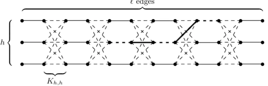
Fig. 1.The graphGh,and an augmenting path.
describes whether the corresponding edge is chosen. Finally, fG(E) = |E|, if the edges of E are a G-matching, and fG(E) = 0 otherwise. A search heuris- tic can start with the empty matching. We investigate three randomized search heuristics. Randomized local search RLS flips a coin in order to decide whether it flips one or two bits uniformly at random. It is obvious that an RLS flipping only one bit per step can get stuck in local optima. Flipping two bits in a step, an augmenting path can be shortened by two edges within one step. If the aug- menting path has length 1, the matching can be enlarged by flipping the edge on this path. The mutation operator EA flips each bit independently with probabil- ity 1/m. This allows to flip all bits of an augmenting path simultaneously. The analysis of EA is much more difficult than the analysis of RLS since more global changes are possible. Finally, SA is some standard form of simulated annealing whose details are not described here (see Sasaki and Hajek (1988)).
Practitioners do not ask for optimal solutions, they are satisfied with (1 +ε)- optimal solutions, in particular, if they can choose the accuracy parameterε >0.
It is sufficient to find a (1 +ε)-optimal solution in expected polynomial time and to obtain a probability of 3/4 of finding a (1 +ε)-optimal solution within a poly- nomial number of steps. Algorithms with the second property are called PRAS (polynomial-time randomized approximation scheme). Giel and Wegener (2003) have shown that RLS and EA have the desired properties and the expected run time is bounded byO(m21/ε). This question has not been investigated for SA.
The observation is that small matchings imply the existence of short augmenting paths. For RLS the probability of a sequence of steps shortening a path to an augmenting edge is estimated. For EA it is sufficient to estimate the probability of flipping exactly all the edges of a short augmenting path. These results are easy to prove and show that randomized search heuristics perform quite well for all graphs.
The run time grows exponentially with 1/ε. This is necessary as the following example shows (see Figure 1). The graphGh,hash·(+ 1) nodes arranged as h×(+ 1)-grid. All “horizontal” edges exist. Moreover, the columns 2i and 2i+ 1 are connected by all possible edges. The graph has a unique perfect matching consisting of all edges ((i,2j−1),(i,2j)). Figure 1 shows an almost perfect matching (solid edges). In such a situation there is a unique augmenting
path which goes from left to right perhaps changing the row, in our example (2,5),(2,6),(2,7),(2,8),(1,9),(1,10). The crucial observation is that the free node (2,5) (similarly for (1,10)) is connected to h+ 1 free edges whose other endpoints are connected to a unique matching edge each. There areh+ 1 2-bit- flips changing the augmenting path at (2,5),hof them increase the length of the augmenting path and only one decreases the length. If h≥2, this is an unfair game and we may conjecture thatGh,,h≥2, is difficult for randomized search heuristics.
This is indeed the case. Sasaki and Hajek (1988) have proved for SA that the expected optimization time grows exponentially ifh=. Giel and Wegener (2003) have proved a bound of 2Ω()on the expected optimization time for each h≥2 and RLS and EA. The proof for RLS follows the ideas discussed above.
One has to be careful since the arguments do not hold if an endpoint of the augmenting path is in the first or last column. Moreover, we have to control which matchings are created during the search process. Many of the methods discussed in Section 3 are applied, namely typical runs analyzed with appropriate potential functions (length of the shortest augmenting path), drift analysis, gambler’s ruin problem, and Chernoff bounds. The analysis of EA is even more difficult. It is likely that there are some steps where more than two bits flip and the resulting bit string describes a matching of the same size. Such a step may change the augmenting paths significantly. Hence, a quite simple, bipartite graph where the degree of each node is bounded above by 3 is a difficult problem instance for typical search heuristics.
Our arguments do not hold in the caseh= 1, i.e., in the case that the graph is a path of odd length. In this case, RLS and EA find the perfect matching in an expected number of O(m4) steps (Giel and Wegener (2003)). One may wonder why the heuristics are not more efficient. Consider the situation of one augmenting path of length Θ() = Θ(m). Only four different 2-bit-flips are accepted (two at each endpoint of the augmenting path). Hence, on the average only one out ofΘ(m2) steps changes the situation. The length of the augmenting path has to be decreased by Θ(m). The “inverse” of Chernoff’s bound (see Section 3) implies that we need on the averageΘ(m2) essential steps. The reason is that we cannot decrease the length of the augmenting path deterministically.
We play a coin tossing game and have to wait until we have wonΘ(m) euros.
We cannot lose too much since the length of the augmenting path is bounded above bym.
The considerations show that randomized search heuristics “work” at free nodes v. The pairs ((v, w),(w, u)) of a free and a matching edge cannot be distinguished by black-box heuristics with small space bounds. Some of them will decrease and some of them will increase the length of augmenting paths.
If this game is fair “on the average”, we can hope to find a better matching in expected polynomial time. Which graphs are fair in this imprecise sense?
There is a new result of Giel and Wegener showing that RLS finds an optimal matching in trees withnnodes in an expected number ofO(n6) steps. One can construct situations which look quite unfair. Then nodes have a large degree.
Trees with many nodes of large degree have a small diameter and/or many leaves. A leaf, however, is unfair but in favor of RLS. If a leaf is free, a good 2-bit-flip at this free node can only decrease the length of each augmenting path containing the leaf. The analysis shows that the bad unfair inner nodes and the good unfair leaves together make the game fair or even unfair in favor of the algorithm.
8 Population-Based Search Heuristics and Search with Crossover
We have seen that randomized local search RLS is often efficient. RLS is not able to escape from local optima. This can be achieved with the same search operator if we accept sometimes worsenings. This idea leads to the Metropolis algorithm or simulated annealing. Another idea is the mutation operator EA from evolutionary algorithms. It can perform non-local changes but it prefers local and almost local changes. In any case, these algorithms work with a space restriction of 1.
One of the main ideas of evolutionary algorithms is to work with more search points in the storage, typically called population-based search. Such a population can help only if the algorithm maintains some diversity in the population, i.e., it contains search points which are not close together. It is not necessary to define these notions rigorously here. It should be obvious nevertheless that it is more difficult to analyze population-based search heuristics (with the exception of multi-start variants of simple heuristics).
Moreover, the crossover operator needs a population. We remember that crossover creates a new search point z from two search points xand y. In the case of Sn ={0,1}n, one-point crossover choosesi ∈ {1, . . . , n−1} uniformly at random and z = (x1, . . . , xi, yi+1, . . . , yn). Uniform crossover decides with independent coin tosses whether zi = xi or zi = yi. Evolutionary algorithms where crossover plays an important role are called genetic algorithms. There is only a small number of papers with a rigorous analysis of population-based evolutionary algorithms and, in particular, genetic algorithms.
The difficulties can be described by the following example. Assume a popula- tion consisting ofnsearch points all havingkones where k > n/2. The optimal search point consists of ones only, all search points with k ones are of equal fitness, and all other search points are much worse. Ifkis not very close ton, it is quite unlikely to create 1n with mutation. A genetic algorithm will sometimes choose one search point for mutation and sometimes choose two search points x and y for uniform crossover and the resulting search point z is mutated to obtain the new search pointz∗. Uniform crossover can create 1n only if there is no position i wherexi =yi = 0. Hence, the diversity in the population should be large. Mutation creates a new search point close to the given one. If both stay in the population, this can decrease the diversity. Uniform crossover creates a search point z betweenxand y. This implies that the search operators do not support the creation of a large diversity. Crossover is even useless if all search
points of the population are identical. In the case of a very small diversity, mu- tation tends to increase the diversity. The evolution of the population and its diversity is a difficult stochastic process. It cannot be analyzed completely with the known methods (including rapidly mixing Markoff chains). Jansen and We- gener (2002) have analyzed this situation. In the case ofk=n−Θ(logn) they could prove that a genetic algorithm reaches the goal in expected polynomial time. This genetic algorithm uses standard parameters with the only exception that the probability of performing crossover is very small, namely 1/(cnlogn) for some constantc. This assumption is necessary for the proof that we obtain a population with quite different search points.
Since many practitioners believe that crossover is essential, theoreticians are interested in proving this, i.e., in proving that a genetic algorithm is efficient in situations where all mutation- and population-based algorithms fail. The most modest aim is to prove such a result for at least one instance of one perhaps even very artificial problem. No such result was known for a long time. The royal road functions (see Section 4) were candidates for such a result. We have seen that randomized local search and simple evolutionary algorithms solve these problems in expected time O((n/d)·log(n/d+ 1)·2d) and the black-box complexity of these problem isΩ(2d) (see Section 9). Hence, there can be no superpolynomial trade-off for these functions. The first superpolynomial trade-off has been proved by Jansen and Wegener (2002, the conference version has been published 1999) based on the results discussed above. Later, Jansen and Wegener (2001a) have designed artificial functions and have proved exponential trade-offs for both types of crossover.
9 Results on the Black-Box Complexity of Specific Problems
We have seen that all typical randomized search heuristics work in the black- box scenario and they indeed work with a small storage. Droste, Jansen, and Wegener (2003) have proved several lower bounds on the black-box complex- ity of specific problems. The lower-bound proofs apply Yao’s minimax principle (Yao (1977)). Yao considers the zero-sum game between Alice choosing a prob- lem instance and Bob choosing an algorithm (a decision tree). Bob has to pay for each query asked by his decision tree when confronted with the problem instance chosen by Alice. Both players can use randomized strategies. If the number of problem instances and the number of decision trees are finite, lower bounds on the black-box complexity can be obtained by proving lower bounds for determin- istic algorithms for randomly chosen problem instances. We are free to choose the probability distribution on the problem instances.
The following application of this technique is trivial. Let Sn be the search space and letfa,a∈Sn, be the problem instance wherefa(a) = 1 andfa(b) = 0 for b=a. The aim is maximization. We choose the uniform distribution on all fa,a∈Sn. A deterministic decision tree is essentially a decision list. If a query leads to the answer 1, the search is stopped successfully. Hence, the expected
depth is always at least (|Sn|+ 1)/2 and this bound can be achieved if we query alla∈Sn in random order.
This example seems to be too artificial to have applications. The shortest- paths problem (see Section 6) with a single objective contains this problem where the search space consists of all trees rooted at s. Hence, we know that this problem is hard in black-box optimization. In the case of the maximization of monotone polynomials we have the subproblem of the maximization of all z1· · ·zd where zi ∈ {xi,1−xi}. The bits at the positionsd+ 1, . . . , n have no influence on the answers to queries. Hence, we get the lower bound (2d+ 1)/2 for the maximization of polynomials (or monomials) of degreed. This bound is not far from the upper bound shown in Section 4.
For several problems, we need lower bounds which hold only in a space- restricted scenario since there are small upper bounds in the unrestricted sce- nario:
– O(n) for sorting and the distance measure INV,
– O(nlogn) for sorting and the distance measures HAM and RUN,
– O(n) for shortest paths as multi-objective optimization problem (a simula- tion of Dijkstra’s algorithm),
– O(m2) for the maximum matching problem.
Finally, we discuss a non-trivial lower bound in black-box optimization. A function is unimodal on {0,1}n if each non-optimal search point has a better Hamming neighbor. It is easy to prove that RLS and EA can optimize unimodal functions with at most b different function values in an expected number of O(nb) steps. This bound is close to optimal. A lower bound of Ω(b/nε) has been proved by Droste, Jansen, and Wegener (2003) if (1 +δ)n≤b= 2o(n)(an exponential lower bound for deterministic algorithms has been proven earlier by Llewellyn, Tovey, and Trick (1989)). Here the idea is to consider the following stochastic process to create a unimodal function. Set p0 = 1n, let pi+1 be a random Hamming neighbor of pi, 1 ≤ i ≤ b−n. Then delete the circles on p0, p1, . . .to obtain a simple pathq0, q1, . . .. Finally, letf(qi) =n+iandf(a) = a1 +· · ·+an for all a outside the simple path. Then it can be shown that a randomized search heuristic cannot do essentially better than to follow the path.
Conclusion
Randomized search heuristics find many applications but the theory of these heuristics is not well developed. The black-box scenario allows the proof of lower bounds for all randomized search heuristics – without complexity theoretical as- sumption. The reason is that the scenario restricts the information about the problem instance. Moreover, methods to analyze typical heuristics on optimiza- tion problems have been presented. Altogether, the idea of a theory of random- ized search heuristics developed as well as the theory of classical algorithms is still a vision but steps to approach this vision have been described.
References
1. Dietzfelbinger, M., Naudts, B., van Hoyweghen, C., and Wegener, I. (2002). The analysis of a recombinative hill-climber on H-IFF. Submitted for publication in IEEE Trans. on Evolutionary Computation.
2. Droste, S., Jansen, T., and Wegener, I. (2003). Upper and lower bounds for ran- domized search heuristics in black-box optimization. Tech. Rep. Univ. Dortmund.
3. Droste, S., Jansen, T., and Wegener, I. (2002). On the analysis of the (1+1) evolu- tionary algorithm. Theoretical Computer Science 276, 51–81.
4. Giel, O. and Wegener, I. (2003). Evolutionary algorithms and the maximum match- ing problem. Proc. of 20th Symp. on Theoretical Aspects of Computer Science (STACS), LNCS 2607, 415–426.
5. Glover, F. and Laguna, M. (1993). Tabu search. In C.R. Reeves (Ed.): Modern Heuristic Techniques for Combinatorial Problems,70–150, Blackwell, Oxford.
6. Hajek, B. (1982). Hitting-time and occupation-time bounds implied by drift analysis with applications. Advances in Applied Probability 14, 502–525.
7. He, J. and Yao, X. (2001). Drift analysis and average time complexity of evolutionary algorithms. Artificial Intelligence 127, 57–85.
8. Jansen, T. and Wegener, I. (2001a). Real royal road functions — where crossover provably is essential. Proc. of 3rd Genetic and Evolutionary Computation Conf.
(GECCO), 375–382.
9. Jansen, T. and Wegener, I. (2001b). Evolutionary algorithms — how to cope with plateaus of constant fitness and when to reject strings of the same fitness. IEEE Trans. on Evolutionary Computation 5, 589–599.
10. Jansen, T. and Wegener, I. (2002). The analysis of evolutionary algorithms — a proof that crossover really can help. Algorithmica 34, 47–66.
11. Kirkpatrick, S., Gelatt, C.D., and Vecchi, M.P. (1983). Optimization by simulated annealing. Science 220, 671–680.
12. Llewellyn, D.C., Tovey, C., and Trick, M. (1989). Local optimization on graphs.
Discrete Applied Mathematics 23, 157–178.
13. Lov´asz, L., Naor, M., Newman, I., and Wigderson, A. (1991). Search problems in the decision tree model. Proc. of 32nd IEEE Symp. on Foundations of Computer Science (FOCS), 576–585.
14. Papadimitriou, C.H., Sch¨affer, A.A., and Yannakakis, M. (1990). On the complexity of local search. Proc. of 22nd ACM Symp. on Theory of Computing (STOC), 438–445.
15. Rabani, Y., Rabinovich, Y., and Sinclair, A. (1998). A computational view of population genetics. Random Structures and Algorithms 12, 314–330.
16. Ranade, A.G. (1991). How to emulate shared memory. Journal of Computer and System Sciences 42, 307–326.
17. Sasaki, G. and Hajek, B. (1988). The time complexity of maximum matching by simulated annealing. Journal of the ACM 35, 387–403, 1988.
18. Scharnow, J., Tinnefeld, K., and Wegener, I. (2002). Fitness landscapes based on sorting and shortest paths problems. Proc. of 7th Conf. on Parallel Problem Solving from Nature (PPSN–VII), LNCS 2439, 54–63.
19. Wegener, I. (2001). Theoretical aspects of evolutionary algorithms. Proc. of 28th Int. Colloquium on Automata, Languages and Programming (ICALP), LNCS 2076, 64–78.
20. Wegener, I. and Witt, C. (2003). On the optimization of monotone polynomials by simple randomized search heuristics. Combinatorics, Probability and Computing, to appear.
21. Yao, A.C. (1977). Probabilistic computations: Towards a unified measure of com- plexity. Proc. of 17th IEEE Symp. on Foundations of Computer Science (FOCS), 222–227.