A framework for the study of physical conditions in astrophysical plasmas through radio and
optical polarization
Application to extragalactic jets
INAUGURAL-DISSERTATION
zur
Erlangung des Doktorgrades
der Mathematisch-Naturwissenschaftlichen Fakultät der Universität zu Köln
vorgelegt von Ioannis Myserlis
aus Thessaloniki, Griechenland
Köln 2015
Tag der letzten mündlichen Prüfung: 30. Oktober 2015
iii
A BSTRACT
This work presents a framework for the study of the physical conditions in astrophysical plasma elements through linear and circular, radio and optical polarization monitoring. The term
“framework” is meant to describe the self-consistent character of the work which contains all necessary elements to:
1. Design and conduct high-cadence, multi-frequency polarimetric observations.
2. Reconstruct the Stokes 4-vector of the observed radiation with high accuracy.
3. Interpret polarimetric observations based on the theoretical predictions of several emis- sion, absorption and propagation effects which can generate, modify, or eliminate the Stokes parameters of the radiation.
4. Reproduce the observed characteristics in the complete Stokes parameters set using a radiative transfer code we developed on the basis of the model of Hughes et al. (1989a).
The development of the machinery of this framework was based on data obtained within the F-GAMMA monitoring program. Our polarimetric methodology eliminates a number of sources of uncertainty and is directly applicable to radio telescopes equipped with circularly polarized feeds.
Using this methodology we recovered the polarization characteristics for a sample of 87 AGNs at 4 bands: 2.64, 4.85, 8.35 and 10.45 GHz. Our analysis focuses on observations conducted with the 100-m Effelsberg telescope between July 2010 and January 2015 with a mean cadence of 1.6 months.
We used these datasets to characterize the observed sample in terms of linear and circular radio polarization. The computed polarization parameters were subsequently used as the basis for the computation of the magnetic field strength of those jets and the rotation measure which is attributed to the low energy magnetized plasma located in regions where the radiation is emitted or propagated through. The theoretical predictions for the emission, absorption and propagation of radiation were used to perform a thorough correlation analysis between several observed characteristics in order to investigate the physical conditions of the emitting plasma elements.
Multi-frequency, high cadence observations are essential in the study of the pronounced variability these sources usually show. This variability was found to follow repeating pat- terns in the F ν –ν domain for many sources, a prototype of which is the blazar 3C 454.3.
In many cases, these patterns agree with the predictions of the “shock-in-jet” model (Marscher and Gear, 1985) which attributes them to the evolution of physical conditions at shocked regions as they propagate downstream the jet. Our results showed coordinated changes of the polarization characteristics which mark the transitions between the optically thick and thin regimes of synchrotron emission. Assuming that these transitions are due to the opti- cal depth evolution of the propagated shocks, we used our radiative transfer code to emulate them and reproduce the variability observed in all Stokes parameters in the case of the proto- type source 3C 454.3. We followed the strict requirement to reproduce this variability just by evolving the physical characteristics of the emitting region according to the predictions of the
“shock-in-jet” model. This approach resulted in a number of estimates for the physical condi- tions of this jet, like its particle number density, magnetic field coherence length and Doppler factor.
Finally, we characterized our sample in terms of optical linear polarization using the data
obtained with the RoboPol monitoring program between May 2013 and July 2015. The com-
parison of those partially simultaneous, radio and optical polarization datasets did not show
any correlation between the two bands, suggesting that the physical conditions at the two emis-
sion sites are different. We detected 60 EVPA rotation events in the examined radio bands, that
occurred in 22 sources of our sample, 6 of which have also shown such events in the optical
wavelengths. Assuming that these rotations are caused by the helical motion of emission el- ements propagating downstream the jet, we used the rotation rates and the linear polarization degree measurements in both the radio and optical bands to compare the (tangential) velocities and hence the kinetic energies of those emission elements while they are propagating through the radio and optical emission sites in the jet.
This thesis is structured as follows; In Chapter 1 we give a brief overview of the AGN struc-
ture and the theoretical predictions for the polarization properties necessary throughout the rest
of the thesis. In Chapters 2 and 3 we describe the machinery of our framework used to extract
and calibrate all the Stokes parameters for radio telescopes equipped with circularly polarized
feeds. In Chapter 4 we characterize the linear and circular radio polarization properties of our
sample of AGNs. Those are later used to calculate other physical parameters at the emission or
propagation regions and to perform a correlation analysis investigating the underlying physical
mechanisms. In Chapter 5 we describe our radiative transfer code and its application on the
radio polarimetric data of 3C 454.3 to reproduce the observed variability and extract a number
of its physical parameters. In Chapter 6 we characterize the optical polarization properties of
our sample, correlate them with the ones found in the radio bands and use the combined in-
formation to compare the physical conditions in the two emission sites in the jet. Finally, in
Chapter 7, we summarize the results and conclusions reached throughout this thesis.
v
K URZZUSAMMENFASSUNG
Diese Arbeit präsentiert ein Rahmenwerk zur Studie physikalischer Zustände in astro- physikalischen Plasmaelementen durch die langfristige Beobachtung linearer und zirkularer Polarisation im Radio- und optischen Wellenlängenbereich. Der Begriff “Rahmenwerk” soll hierbei den selbstkonsistenten Charakter dieser Arbeit verdeutlichen, welche alle nötigen Ele- mente enthält um:
1. Polarisationsmessungen in mehreren Frequenzbändern mit hoher Beobachtungsrate zu konzipieren und durchzuführen;
2. Den Stokes-4-Vektor der beobachteten Strahlung mit hoher Genauigkeit zu rekonstru- ieren;
3. Polarisationsdaten basierend auf den theoretischen Vorhersagen verschiedener Emissions-, Absorptions-, und Ausbreitungsmechanismen zu interpretieren, welche die Stokes-Parameter generieren, modifizieren oder auslöschen können;
4. Die beobachteten Charakteristika des vollständigen Stokes-Vektors mittels eine Strahlungstransfer-Codes zu reproduzieren, welcher auf der Basis des Models von Hughes et al. (1989a) im Rahmen dieser Arbeit entwickelt wurde.
Die Basis zur Entwicklung der Methodik dieses Rahmenwerks bilden Daten, die als Teil des F-GAMMA Beobachtungsprogramms gemessen wurden. Die hier beschriebene Methodik eliminiert eine Reihe von Fehlerquellen und lässt sich direkt auf beliebige Radioteleskope an- wenden, welche mit zirkular polarisiertem Feed ausgerüstet sind.
Durch die Anwendung dieser Methode wurden die Polarisationscharakteristika von 87 ak- tiven Galaxienkernen in vier Frequenzbändern rekonstruiert: 2,64, 4,85, 8,35 und 10,45 GHz.
Die entsprechenden Daten wurden mit dem Effelsberg-100m-Teleskop zwischen Juli 2010 und Januar 2015 mit einer mittleren Wiederholungsrate von 1,6 Monaten gemessen.
Basierend auf diesen Daten wurden die linearen und zirkularen Polarisationszustände der Objekte in der Stichprobe untersucht. Die erhaltenen Polarisationsparameter wurden daraufhin verwendet, um die magnetische Feldstärke dieser Jets zu errechnen sowie das Rotationsmaç, welches auf das niedrigenergetische, magnetisierte Plasma zurückzuführen ist, welches sich in den Regionen befindet, in denen die Strahlung erzeugt oder durch diese transmittiert wird.
Theoretische Vorhersagen über die Emission, Absorption und Transmission wurden verwendet, um verschiedene Kombinationen von gemessenen Grössen auf Korrelationen zu untersuchen, um Rückschlüsse auf das emittierende Plasmaelement zu ziehen.
Wiederholte Beobachtungen in mehreren Frequenzbändern in kurzen Zeitintervallen sind
nötig, um die ausgeprägte Variabilität, die diese Objekte typischerweise zeigen, untersuchen zu
können. Es ist bekannt, dass diese Variabilität einem wiederholenden Muster im F ν –ν-Raum
folgt. Blazar 3C 454.3 ist hierfür ein Prototyp. In vielen Fällen stimmt dieses Muster mit den
Vorhersagens des “shock-in-jet”-Modells (Marscher and Gear, 1985) überein, welches dieses
auf die Entwicklung des physikalischen Zustandes der schockkomprimierten Region zurück-
führt, während diese durch den Jet propagiert. Hier präsentierte Resultate zeigen schematische
Änderungen des Polarisationszustandes, welche den Übergang von der optisch dicken zur op-
tisch dünnen Synchrotronemission darstellen. Unter der Annahme, dass diese Übergänge durch
die Änderung der optischen Tiefe des propagierenden Schocks beschrieben werden können,
wurde für das Objekt 3C 454.3 ein Strahlungstransfer-Code angewendet, um die beobachtete
Variation in allen vier Stokes-Parametern nachzubilden. Hierbei wurde der strikten Bedingung
Folge geleistet, dass die beobachtete Variation lediglich aus der Entwicklung der physikalis-
chen Charakteristika der Emissionsregion resultiert, gemäss den Vorhersagen des “shock-in-
jet”-Modells. Aus diesem Ansatz resultiert die Schätzung einer Reihe von physikalischen Pa-
rametern, darunter die Partikelanzahldichte, die Kohärenzlänge des magnetischen Feldes und
der Dopplerfaktor des Jets.
Des Weiteren wurde die lineare Polarisation im optischen Frequenzbereich der gesamten Objektstichprobe untersucht, basierend auf den Daten, die im Rahmen des RoboPol Beobach- tungsprogramms zwischen May 2013 und Juli 2015 gemessen wurden. Der Vergleich der zum Teil zeitgleichen Daten im optischen und im Radiobereich zeigte keinerlei Korrelation zwischen den zwei Frequenzbändern. Dies deutet darauf, dass die physikalischen Bedingun- gen in den zwei Emissionsregionen verschieden sind. Insgesamt 60 EVPA-Rotationen wur- den in den untersuchten Frequenzbändern beobachtet. Diese traten in 22 Objekten aus der gesamten Stichprobe auf, sechs davon zeigten ebenfalls Rotationen im optischen Wellenlän- genbereich. Unter der Annahme, dass diese Rotationen aus der Bewegung von spiralförmig durch den Jet propagierenden Emissionselementen resultiert, wurden die Rotationsraten und der lineare Polarisationsgrad in beiden Frequenzbereichen verwendet, um die (tangentialen) Geschwindigkeiten und somit die kinetische Energie der Emissionselemente zu vergleichen, während diese durch das Radio- bzw. optische Emissionsgebiet propagieren.
Diese Arbeit gliedert sich wie folgt: Kapitel 1 gibt eine kurze Einleitung in die Struktur von aktiven Galaxienkernen und theoretische Vorhersagen über die Polarisationseigenschaften, die in der weiteren Arbeit benötigt werden. In den Kapiteln 2 und 3 wird die Methodologie zur Kalibrierung und Messung von Stokes-Parametern für mit zirkular polarisierten Feeds aus- gestattete Radioteleskope beschrieben. In Kapitel 4 werden die linearen und zirkularen Polari- sationseigenschaften der untersuchten Stichprobe von aktiven Galaxienkernen charakterisiert.
Diese Ergebnisse werden dann verwendet, um zum einen weitere physikalische Parameter der Emissionsregion abzuleiten, zum anderen mittels Korrelationsanalyse die grundlegenden physikalischen Mechanismen zu untersuchen. In Kapitel 5 wird der Strahlungstransfer-Code beschrieben und auf die polarimetrischen Daten von 3C 454.3 angewandt, um die beobachtete Variabilität zu rekonstruieren und daraus verschiedene physikalische Parameter abzuleiten.
Die optischen Polarisationseigenschaften der untersuchten Stichprobe von Objekten werden
in Kapitel 6 untersucht und mit den entsprechenden Radiopolarisationsdaten korreliert, um die
physikalischen Bedingungen der beiden Emissionsregionen im Jet, verantwortlich für die op-
tische und die Radio-Emission, zu vergleichen. Zuletzt werden die Ergebnisse und Schlussfol-
gerungen dieser Arbeit in Kapitel 7 zusammengefasst.
vii
A CKNOWLEDGEMENTS
This work would not have been completed without the essential contribution of many people who I would like to acknowledge here.
First and foremost I would like to express my sincere gratitude to my PhD adviser Dr.
Emmanouil (Manolis) Angelakis for his continuous support, patience and motivation. Our frequent, thorough and multi-disciplinary discussions had a deep impact on this work, my scientific and personal development throughout the last three years. I could not have imagined having a better adviser and mentor for my PhD study.
I would like to express the deepest appreciation to my supervisors. First, to the director of the VLBI group at the Max Planck Institute for Radio Astronomy, Prof. Dr. J. Anton Zensus, for his support in a number of ways and his insightful comments and encouragement. I would also like to express my gratitude to Prof. Dr. Andreas Eckart at the I. Physikalisches Institut for reviewing this work.
Moreover, I appreciate the feedback offered by the other members of my thesis advisory committee: Dr. Alex Kraus for his suggestions and comments which were invaluable for the completion of this thesis, Prof. Vasiliki Pavlidou for her dedicated encouragement and guidance as well as Dr. Lars Fuhrmann for his constructive comments.
I want to thank all the members of the VLBI group which provided a productive environ- ment to conduct research and our secretary Frau Beate Naunheim for her prompt support. My sincere thanks goes to Dr. Richard Porcas for our many fruitful and stimulating discussions.
I am also grateful to all the members of the RoboPol collaboration. Being part of such an international collaboration has been a very inspiring experience. Special thanks goes to Prof. A. N. Ramaprakash, Prof. Iossif Papadakis, Dr. Oliver G. King, Dr. Dmitry Blinov, Dr. Talvikki Hovatta and Dr. Pablo Reig for having numerous stimulating and constructive discussions.
A large part of this work is based on observations with the 100-m telescope of the MPIfR (Max-Planck-Institut für Radioastronomie) at Effelsberg. Thus, my thanks goes also to the personnel of the telescope who were always very helpful, keeping me company during the long nights of observations and supporting in any way possible. Advice and comments given by Dr. Peter Müller has been a great help in discovering the workings of the 100-m telescope.
I express my gratitude also to all friends and colleagues who made my PhD life easier and pleasant: Vassilis Karamanavis, Ioannis Antoniadis, Ioannis Nestoras, Sebastian Kiehlmann, Jeffrey Hodgson, Florent Mertens, Bindu Rani, Biaginna Boccardi, Behnam Javanmardi, Fateme Kamali, Miguel Requena Torres, Macarena García-Marín, Kostas Markakis, Anastasia Tsitali and Dhanya Nair.
I thank also the administration of the International Max Planck Research School for As- tronomy and Astrophysics. Both the coordinators Dr. Emmanouil Angelakis and Priv.-Doz.
Dr. Rainer Mauersberger as well as their assistant Dr. Simone Pott were always caring and made studying in Germany a creative learning experience.
I owe my deepest gratitude to my first mentor Prof. John H. Seiradakis at the Aristotle University of Thessaloniki for enlightening me at the first steps of research and Dr. Anastasios Molochidis for showing me the beauty of natural sciences.
Finally, I would like to thank my parents Valia and Grigorios as well as my siblings Evi,
Pavlos and Ilias for the continuous support they have given me as well as my soul mate Hariklia
for her caring love and patience throughout this effort.
Contents viii
List of Figures xi
List of Tables xv
1 Synchrotron emission and radiative transfer 1
1.1 Active Galactic Nuclei: The big picture . . . . 1
1.1.1 The “central engine” and the obscuring torus . . . . 1
1.1.2 The narrow and broad line regions . . . . 2
1.1.3 The jet . . . . 3
1.2 Synchrotron emission . . . . 5
1.2.1 Emission from a single particle . . . . 5
1.2.2 Emission and absorption from an ensemble of particles . . . . . 10
1.2.3 Self-absorption . . . . 11
1.2.4 Emission and absorption for an ensemble of particles with power law energy distribution . . . . 12
1.2.5 Emission and absorption from an ensemble of mildly relativistic particles . . . . 15
1.3 Polarized radiative transfer . . . . 17
1.4 Propagation effects . . . . 19
1.4.1 Synchrotron Self Absorption (SSA) and polarization characteristics 21 1.4.2 Faraday rotation . . . . 23
1.4.3 Faraday pulsation . . . . 23
1.4.4 Circular repolarization . . . . 25
1.5 From the source to the observer’s rest frame . . . . 25
2 High precision, full-Stokes radio polarimetry 29 2.1 The method . . . . 29
2.2 The R matrix . . . . 30
2.3 The M matrix . . . . 33
2.4 The measured Stokes vector . . . . 34
2.4.1 Stokes parametrization for circularly polarized feeds . . . . 36
2.4.2 Extracting the observables . . . . 36
2.4.3 Cross-channel calibration . . . . 38
2.4.4 Corrections . . . . 42
2.4.5 Stokes Q and U instrumental artifacts . . . . 50
3 Full-Stokes polarimetry calibration 59 3.1 Introduction . . . . 59
viii
CONTENTS ix
3.2 Full-Stokes calibration techniques . . . . 59
3.2.1 4x4 Müller matrix calibration . . . . 59
3.2.2 Full-Stokes sensitivity calibration . . . . 60
3.2.3 Our approach . . . . 60
3.3 Stokes V calibration . . . . 61
3.4 System stability . . . . 63
4 Radio linear and circular polarization of AGN jets 67 4.1 Introduction . . . . 67
4.2 The dataset . . . . 67
4.2.1 Quality Checks and data operations . . . . 68
4.2.2 Demographics of polarized sources . . . . 72
4.2.3 Linearly and circularly-only polarized sources . . . . 72
4.2.4 Linear polarization per observing frequency . . . . 73
4.2.5 Circular polarization per observing frequency . . . . 74
4.2.6 Polarized state duration . . . . 74
4.2.7 Total flux and linear polarization spectra . . . . 74
4.3 Derivative quantities . . . . 79
4.3.1 Magnetic field magnitude . . . . 79
4.3.2 Rotation measure . . . . 82
4.4 Correlation analysis . . . . 85
4.4.1 EVPA versus AGN jet position angle . . . . 87
4.4.2 Linear versus circular polarization degree . . . . 88
4.4.3 Linear and circular polarization versus RM . . . . 90
4.4.4 Polarization degree versus low and high frequency emission characteristics . . . . 90
4.4.5 Polarization characteristics and source type . . . . 94
4.4.6 Polarization degree and flux density state . . . . 97
5 Full-Stokes radiative transfer modelling of shocked jets 103 5.1 Introduction . . . . 103
5.2 Radio variability of AGN jets . . . . 103
5.2.1 The shock-in-jet model . . . . 106
5.2.2 The evolutionary path signature in the polarization characteristics 107 5.3 Full-Stokes radiative transfer code of shocked jets . . . . 107
5.3.1 A short overview of the code . . . . 108
5.3.2 The building blocks of the modeled jet . . . . 108
5.3.3 Full-Stokes radiative transfer . . . . 109
5.3.4 Emulating the jet . . . . 110
5.3.5 Relativistic shock jump conditions . . . . 112
5.4 A study case: the blazar 3C 454.3 . . . . 113
5.4.1 Constraining the jet physical size . . . . 113
5.4.2 Constraining the particle number density . . . . 115
5.4.3 Constraining the number of cells . . . . 115
5.4.4 Reproducing the observed behavior . . . . 116
6 Optical and radio polarization studies of MeV–GeV blazars 119 6.1 Introduction . . . . 119
6.2 Optical polarization data . . . . 119
6.2.1 Demographics . . . . 120
6.2.2 Polarized state duration . . . . 120
6.3 Correlation analysis . . . . 122
6.3.1 Optical linear versus radio linear and circular polarization . . . 122
6.3.2 Optical linear polarization degree against the γ-ray energy flux . 122 6.3.3 Optical linear polarization degree and flux density state . . . . . 122
6.4 Optical and radio EVPA rotations . . . . 125
6.4.1 Optical and radio emission site size from EVPA rotation rates . 128 6.4.2 The kinetic energy ratio between the radio and optical parts of the jet . . . . 128
7 Summary and conclusions 129 7.1 The framework . . . . 129
7.2 High precision linear and circular radio polarimetry . . . . 129
7.3 Linear and circular radio polarization characteristics of AGNs . . . . 130
7.3.1 Linear and circular radio polarization . . . . 131
7.3.2 Derivative quantities . . . . 131
7.3.3 Correlation analysis . . . . 132
7.4 Full-Stokes radiative transfer code . . . . 134
7.4.1 Application to shocked jets . . . . 134
7.4.2 The study case of 3C 454.3 . . . . 134
7.5 Optical polarization properties of AGNs . . . . 135
7.5.1 Optical polarization . . . . 135
7.5.2 Correlation analysis . . . . 136
7.5.3 Optical and radio EVPA rotations . . . . 136
7.6 Future work . . . . 137
A Radio polarization data 139
B Light curves 177
C Spectra 207
D Rotation measure plots 237
E Optical polarization data 253
Bibliography 257
Erklärung 267
Publications / Teilpublikationen 269
List of Figures
1.1 AGN structure . . . . 2
1.2 The SED of 3C279 . . . . 4
1.3 Synchrotron radiation pattern . . . . 7
1.4 Synchrotron emission solid angle . . . . 11
1.5 The functions F (x) and G(x) . . . . 12
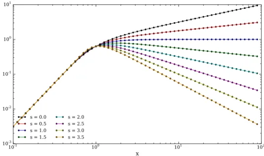
1.6 The J(x, s) function . . . . 14
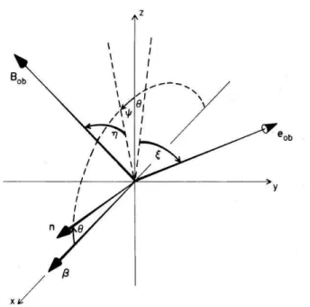
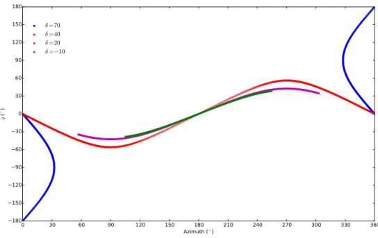
1.7 Relativistic aberration effect on EVPA . . . . 27
2.1 Parallactic angle - azimuth plot for the Effelsberg telescope . . . . 32
2.2 Simulated | ∆Q | and | ∆U | - azimuth plots for two measurement durations with φ = 50 ◦ 31 ′ 29 ′′ and δ = 40 ◦ . . . . 32
2.3 Müller matrix element histograms . . . . 35
2.4 LCP, RCP, COS and SIN channel datasets . . . . 37
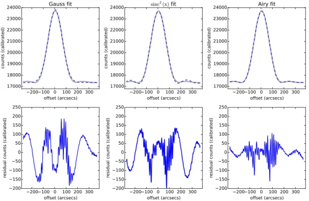
2.5 Fitting method comparison . . . . 39
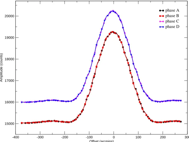
2.6 Phases A - D for the LCP channel . . . . 41
2.7 Differences between the phases recorded by the LCP channel . . . . 42
2.8 Pointing model amplitude improvement . . . . 45
2.9 Channel pointing offsets . . . . 45
2.10 Pointing correction amplitude scatter improvement . . . . 46
2.11 Pointing correction circular polarization degree scatter improvement . . . . . 46
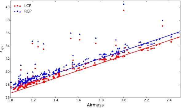
2.12 T sys versus airmass . . . . 49
2.13 Fitted τ z differences between LCP and RCP T sys data . . . . 49
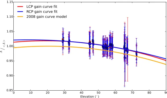
2.14 LCP and RCP channel gain curves . . . . 51
2.15 Stokes Q and U artifacts . . . . 52
2.16 Stokes Q and U artifact correction process . . . . 54
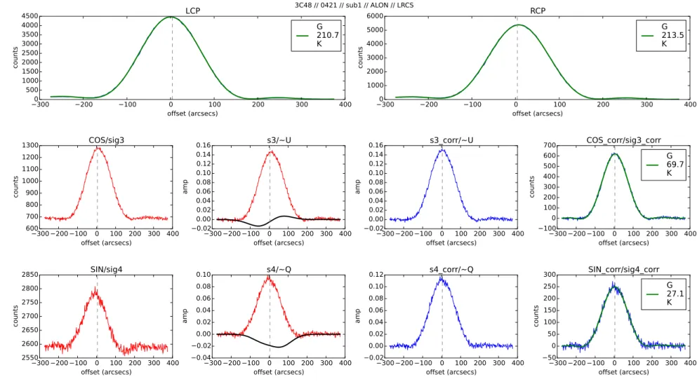
2.17 Linear polarization characteristics of the calibrator 3C 48 before and after the artifact correction . . . . 56
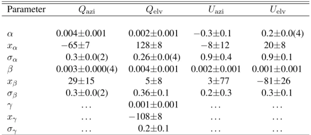
2.18 The generated models of the Stokes Q and U artifacts for 46 consecutive ses- sions. . . . 57
3.1 Uncorrected Stokes V lightcurves . . . . 62
3.2 Sensitivity factors for the 4.85 GHz Effelsberg receiver . . . . 65
3.3 Sensitivity factors for the 8.35 GHz Effelsberg receiver . . . . 66
4.1 Histograms of total flux density for sources with either linear and/or circular polarization . . . . 73
4.2 Histograms of m l . . . . 75
4.3 Histograms of Π l . . . . 76
4.4 Histograms of | m c | . . . . 77
4.5 Histograms of | Π c | . . . . 78
xi
4.6 Histograms of Π l detectability . . . . 78
4.7 Histograms of Π c detectability . . . . 79
4.8 Histograms of B-field strength . . . . 83
4.9 Rotation measure comparison plot . . . . 84
4.10 Histogram of rotation measures . . . . 86
4.11 RM celestial map . . . . 86
4.12 RM vs galactic latitude . . . . 87
4.13 EVPA vs jet PA alignment histogram . . . . 88
4.14 m l vs | m c | . . . . 89
4.15 Median m l vs RM . . . . 91
4.16 Median | m c | vs RM . . . . 92
4.17 Median m l vs γ -ray energy flux . . . . 93
4.18 Median | m c | vs γ-ray energy flux . . . . 94
4.19 Median m l vs synchrotron peak . . . . 95
4.20 Median | m c | vs synchrotron peak . . . . 96
4.21 m l at total flux extrema . . . . 98
4.22 Π l at total flux extrema . . . . 99
4.23 | m c | at total flux extrema . . . . 100
4.24 | Π c | at total flux extrema . . . . 101
5.1 Multi-frequency radio variability of the FSRQ 3C 454.3 . . . . 104
5.2 Multi-frequency radio variability pattern of the blazar 3C454.3 . . . . 105
5.3 "Shock-in-jet" model evolutionary stages . . . . 106
5.4 3C 454.3 Full Stokes lightcurves. . . . 108
5.5 The broadband total flux and polarization characteristics of a synchrotron self- absorbed (SSA) emitting modelled cell as generated with our code. The linear and circular polarization degrees, m l and m c , are normalized to 1. . . . 110
(a) SSA Stokes parameters . . . . 110
(b) SSA polarization characteristics . . . . 110
5.6 A modeled jet profile . . . . 112
5.7 The dependence of the linear polarization degree m l for an optically thin, syn- chrotron emitting compressed plasma cell with tangled magnetic field as a function of the compression factor, k, and the angle between the line of sight and the compression plane, φ (Hughes et al., 1985). . . . 114
(a) m l vs compression k . . . . 114
(b) m l vs angle to compression plane . . . . 114
5.8 The unshocked flow of modeled jet for 3C454.3 . . . . 116
5.9 Simulated Full Stokes lightcurves . . . . 117
6.1 Histogram of optical m l . . . . 121
6.2 Histograms of optical m l detectability . . . . 121
6.3 R band median m l versus radio median m l . . . . 123
6.4 R band median m l versus radio median | m c | . . . . 124
6.5 R band median m l versus γ-ray energy flux . . . . 124
6.6 R-band m l and Π l at low and high flux density state . . . . 125
6.7 Radio EVPA rotation ranges and rates . . . . 126
B.1 Radio linear and circular polarization lightcurves . . . . 178
B.2 continued . . . . 179
B.3 continued . . . . 180
List of Figures xiii
B.4 continued . . . . 181
B.5 continued . . . . 182
B.6 continued . . . . 183
B.7 continued . . . . 184
B.8 continued . . . . 185
B.9 continued . . . . 186
B.10 continued . . . . 187
B.11 continued . . . . 188
B.12 continued . . . . 189
B.13 continued . . . . 190
B.14 continued . . . . 191
B.15 continued . . . . 192
B.16 continued . . . . 193
B.17 continued . . . . 194
B.18 continued . . . . 195
B.19 continued . . . . 196
B.20 continued . . . . 197
B.21 continued . . . . 198
B.22 continued . . . . 199
B.23 continued . . . . 200
B.24 continued . . . . 201
B.25 continued . . . . 202
B.26 continued . . . . 203
B.27 continued . . . . 204
B.28 continued . . . . 205
B.29 continued . . . . 206
C.1 Radio total flux density and linear polarization spectra . . . . 208
C.2 continued . . . . 209
C.3 continued . . . . 210
C.4 continued . . . . 211
C.5 continued . . . . 212
C.6 continued . . . . 213
C.7 continued . . . . 214
C.8 continued . . . . 215
C.9 continued . . . . 216
C.10 continued . . . . 217
C.11 continued . . . . 218
C.12 continued . . . . 219
C.13 continued . . . . 220
C.14 continued . . . . 221
C.15 continued . . . . 222
C.16 continued . . . . 223
C.17 continued . . . . 224
C.18 continued . . . . 225
C.19 continued . . . . 226
C.20 continued . . . . 227
C.21 continued . . . . 228
C.22 continued . . . . 229
C.23 continued . . . . 230
C.24 continued . . . . 231
C.25 continued . . . . 232
C.26 continued . . . . 233
C.27 continued . . . . 234
C.28 continued . . . . 235
C.29 continued . . . . 236
D.1 EVPA versus λ 2 , rotation measure and zero-wavelength EVPA variability plots 238 D.2 continued . . . . 239
D.3 continued . . . . 240
D.4 continued . . . . 241
D.5 continued . . . . 242
D.6 continued . . . . 243
D.7 continued . . . . 244
D.8 continued . . . . 245
D.9 continued . . . . 246
D.10 continued . . . . 247
D.11 continued . . . . 248
D.12 continued . . . . 249
D.13 continued . . . . 250
D.14 continued . . . . 251
D.15 continued . . . . 252
List of Tables
2.1 Fitting method comparison for circular polarization measurements . . . . 38
2.2 The setup of the different phases in the measurement cycle . . . . 40
2.3 LCP and RCP gain curve parameters . . . . 50
2.4 The initial values of the Stokes Q and U artifact model parameters . . . . 53
2.5 Stokes Q and U artifact fitted parameter values . . . . 55
3.1 Calibrated Stokes V and I of standards . . . . 63
3.2 Polarization characteristics of calibrators . . . . 64
4.1 Source list . . . . 69
4.1 continued. . . . 70
4.1 continued. . . . 71
4.2 Demographics of polarized sources . . . . 71
4.3 Linearly and/or circularly polarized sources . . . . 72
4.4 Magnetic field strengths . . . . 80
4.4 continued. . . . 81
4.4 continued. . . . 82
4.5 Rotation measures and 0-wavelength EVPAs . . . . 84
4.5 continued. . . . 85
4.6 FSRQs vs BL Lacs in polarization . . . . 96
4.6 continued. . . . 97
6.1 Demographics of polarized sources in radio and optical . . . . 120
6.2 The list of sources which have shown radio or optical EVPA rotations . . . . 127
A.1 Radio total flux density, linear and circular polarization characteristics . . . . 139
A.1 continued. . . . 140
A.1 continued. . . . 141
A.1 continued. . . . 142
A.1 continued. . . . 143
A.1 continued. . . . 144
A.1 continued. . . . 145
A.1 continued. . . . 146
A.1 continued. . . . 147
A.1 continued. . . . 148
A.1 continued. . . . 149
A.1 continued. . . . 150
A.1 continued. . . . 151
A.1 continued. . . . 152
A.1 continued. . . . 153
xv
A.1 continued. . . . 154
A.1 continued. . . . 155
A.1 continued. . . . 156
A.1 continued. . . . 157
A.1 continued. . . . 158
A.1 continued. . . . 159
A.1 continued. . . . 160
A.1 continued. . . . 161
A.1 continued. . . . 162
A.1 continued. . . . 163
A.1 continued. . . . 164
A.1 continued. . . . 165
A.1 continued. . . . 166
A.1 continued. . . . 167
A.1 continued. . . . 168
A.1 continued. . . . 169
A.1 continued. . . . 170
A.1 continued. . . . 171
A.1 continued. . . . 172
A.1 continued. . . . 173
A.1 continued. . . . 174
A.1 continued. . . . 175
A.1 continued. . . . 176
E.1 Optical polarization characteristics . . . . 253
E.1 continued. . . . 254
E.1 continued. . . . 255
E.1 continued. . . . 256
Chapter 1
Synchrotron emission and radiative transfer
Abstract
In the current thesis, we apply the framework we developed to study the physical conditions in extragalactic jets, hosted by AGNs. Those jets are radiating in the radio and optical bands through the incoherent synchrotron mechanism. In this chapter we give a brief overview of the AGN structure and we provide the theoretical predictions for a number of synchrotron emission, absorption, and propagation effects which can also modify the polarization characteristics. Such effects will be used in the following chapters to interpret the observed behaviour.
The information presented in this chapter is text-book knowledge and can be found at, (e.g. Pacholczyk, 1970, 1977; Ginzburg, 1979; Rybicki and Lightman, 1979). Here we provide it however to establish a common nomenclature throughout this thesis and accu- mulate the part of theory relevant to this work. Most analysis is taken from Pacholczyk (1970) and Pacholczyk (1977).
1.1 A CTIVE G ALACTIC N UCLEI : T HE BIG PICTURE
The term Active Galactic Nucleus (AGN) is used in modern Astrophysics to describe the cen- tral regions of galaxies which exhibit immense energy production. AGNs radiate over an ex- treme range of frequencies with bolometric luminosities higher than their host galaxies up to a factor of ∼ 100. The typical AGN bolometric luminosities are of the order of 10 11 – 10 13 L ⊙ , i.e. ∼ 10 44 – 10 46 erg s −1 (e.g. Peterson, 1997). Furthermore, the AGN emission is highly variable over a very broad range of time scales, from minutes to years. According to coher- ence arguments, the short time scales indicate that most of the radiated energy is produced in a region of linear scale comparable the size of our Solar system. This extreme energy produc- tion in such compact regions supports the current consensus that the energy source of AGNs are supermassive black holes (SMBHs) with masses of the order of 10 9±1 M ⊙ (e.g. Peterson, 1997).
The typical structure of an AGN is shown in Fig. 1.1 and its main constituents are described in the following subsections.
1.1.1 The “central engine” and the obscuring torus
The main energy source – “central engine” – of all AGNs is considered to be a supermas- sive black hole (SMBH) of ∼ 10 9 M ⊙ located at their centes. Its gravitational field accretes matter from the inner part of the host galaxy, surrounding the AGN, and an accretion disk is created as a result of the angular momentum conservation of the infalling material. Part of
1
Figure 1.1: A schematic representation of the AGN structure. The different types of AGN are labeled according to the unification scheme. Figure taken from Beckmann and Shrader (2012)
the gravitational potential energy released through the accretion process is radiated away and the accretion disk becomes extremely hot and luminous due its viscosity. The accretion disk radiation is responsible for the thermal component of the AGN emission and peaks around the extreme ultraviolet and X-ray wavelengths (e.g. Begelman, 1985; Peterson, 1997).
The flow of material onto the SMBH is provided by an optically thick torus which sur- rounds the radiating accretion disk. Depending on the orientation of the AGN with respect to our line of sight (LoS), this torus may obscure the “central engine” from our view.
1.1.2 The narrow and broad line regions
The optical and ultraviolet parts of AGN spectra host a series of broad and narrow lines. Mea- surements of their Full Width at Half Maximum (FWHM) reveal that the regions where broad lines are emitted have average speeds of the level of 5000 km s −1 while the ones producing the narrow lines of the order of 400 km s −1 . Furthermore, in the cases where the “central engine”
was obscured by the torus, the broad lines appeared much fainter and more polarized than the narrow lines (Antonucci and Miller, 1985).
These observations were interpreted as an AGN orientation effect. The broad lines are pro- duced from clouds moving at high velocities because they orbit the SMBH at a close distance.
When the AGN orientation conceals the central region from our LoS, these clouds are not seen directly but only after their emission is scattered in the outer parts of the AGN or the innermost part of the host galaxy. Thus, their lines appear faint and highly polarized due to scattering.
On the other hand, narrow lines are produced by low velocity clouds orbiting the SMBH at
greater distances. They are observed directly independently of the AGN orientation and thus
their lines are not polarized (Antonucci and Miller, 1985).
1.1. ACTIVE GALACTIC NUCLEI: THE BIG PICTURE 3
These findings led to the unification scheme of AGNs (Urry and Padovani, 1995) which attributes the various types of AGN we observe to their orientation with respect to our LoS.
For example, the fact that broad lines are observed for Seyfert 1 but not Seyfert 2 galaxies is explained in this scheme by the obscuration of the central part of the latter type by the torus.
The different classifications of AGN and their explanation according to the unification scheme are shown in Fig. 1.1.
1.1.3 The jet
In about 10 % of AGNs, the so-called radio-loud (RL) ones, a relativistic, collimated, bipo- lar flow of material appears to be ejected from the “central engine”, known as the jet (e.g.
Beckmann and Shrader, 2012). Jets can reach distances of the order of hundreds of kpc or even Mpc and are often terminated in extended regions where material and energy is dissi- pated. Those regions are very bright radio sources, called “hot spots”. Jets appear to be very collimated with opening angles θ ≤ 15 ◦ . Furthermore, the fact that they emit from radio to op- tical or even X-ray wavelengths with the incoherent synchrotron mechanism becomes evident from the continuum, non-thermal appearance of their spectra and the high linear polarization observed (e.g. Boettcher et al., 2012).
Although the composition of jets is an open question, the flow is thought to be described by a charge-neutral plasma of a roughly equal admixture of electrons and protons or electrons and positrons which have similar densities. The typical densities of jets are of the order of 10 −3 − 10 −2 cm −3 (e.g. Begelman et al., 1984). The relativistic motion of jets is supported by a number of observational facts, one of which is that they often appear one-sided. This is attributed to the Doppler beaming effect which enhances the radiation towards the direction of motion of the emitter, due to the relativistic aberration and time dilation effects. Thus, although jet flows are bipolar, in the case of their close alignment with our LoS the flow directed away from us becomes unobservable (e.g. Boettcher et al., 2012).
The spectral energy distributions (SEDs) of AGN jets span from the radio up to TeV ener- gies and contain usually two broad components (Fig. 1.2). The low energy component is at- tributed to the incoherent synchrotron emission of the jet particle population. The strongest ar- gument in favor of this interpretation is the high linear polarization degree observed at these fre- quencies. The high frequency component on the other hand is attributed to two competing inter- pretations or models, the leptonic and the hadronic one. The leptonic model attributes the emis- sion to the inverse Compton up-scattering of the low frequency synchrotron photons to high energies by the relativistic particles that emit them, (e.g. Bednarek et al., 1996). The hadronic model predicts that the high energy photons are produced by electromagnetic cascades which are triggered by photo–pion production from the interaction of ultra-relativistic protons with the ambient synchrotron photons, (e.g. Kazanas and Mastichiadis, 1999; Mücke et al., 2003).
Although the exact processes to form, collimate and sustain jets are not yet fully under-
stood, jets can be adequately described as relativistic magnetized plasma systems. Such sys-
tems are expected to emit radiation with linearly and circularly polarized components (vide
infra). The polarized emission is later propagated through the magnetized jet plasma, i.e. a
magneto-ionic medium which, under certain circumstances, can change its polarization char-
acteristics. The initial polarization state as well as the changes it undergoes as the emission
propagates through the jet are unique probes to estimate many physical parameters of the emit-
ting and transmitting jet plasma. This approach is similar to the techniques used to study many
systems that can not be simulated in vitro (e.g. the Earth’s magma or the Sun’s plasma). The
knowledge of these physical parameters helps to create or improve theoretical jet models by
narrowing their parameter spaces. Furthermore, they offer the potential to investigate the phys-
ical conditions in the vicinity of the AGN’s “central engine” which is physically and causally
connected with the jet itself.
Figure 1.2: The SED of the blazar 3C279. The pronounced variability is evident by the large scatter of data points across the whole electromagnetic spectrum. Figure taken from Boettcher et al. (2012).
Another important characteristic of the AGN jet emission is its pronounced variability across the electromagnetic spectrum, as shown in the example of Fig. 1.2. This variability is often manifested in the synchrotron part of the jet emission by strong flares which are caused by the appearance of SED components at the high frequencies which usually propagate later towards the lower frequencies, (e.g. Marscher and Gear, 1985). These components are often attributed to confined particle “clouds” of higher densities or magnetic field strengths as com- pared to the large scale flow of the jet. Most of the times these particle “clouds” are correlated with localized emission elements in VLBI radio maps of jets. The evolution of their physical characteristics as they propagate downstream the jet is imprinted on their spectral variability as well the changes of their polarization state. Thus, multi-frequency, high cadence observations of their total flux and polarization are powerful probes to study the physical parameters of these systems.
This work is concentrated on the study of the AGN jet emission and variability in the radio
and optical parts of the electromagnetic spectrum by means of high cadence, multi-frequency
linear and circular radio as well as linear optical polarimetry. We exploit the invaluable tool of
polarimetry primarily because such information are a direct measure of the physical parameters
of the emitting regions, like their magnetic field strength and uniformity. In the following
sections, we will describe the emission processes which produce the polarized radio and optical
jet radiation as well as the effects which can potentially change the polarization characteristics
of the emission during its propagation through the jet’s magnetized plasma.
1.2. SYNCHROTRON EMISSION 5
1.2 S YNCHROTRON EMISSION
As discussed above, we focus on the radio and optical parts of the AGN jet emission, consid- ered to be generated by the incoherent synchrotron mechanism. In this section, we describe briefly the synchrotron emission from a single particle as well as from an ensemble of particles embedded in large scale magnetic fields. This setup can be considered as the first order approx- imation of a synchrotron emitting AGN jet as well as the high density "clouds" which cause the flaring behavior as described in subsection 1.1.3. The predictions of synchrotron theory presented here provide a link between the physical conditions of the emitting regions and the total flux as well as linear and circular polarization characteristics of the emitted radiation.
The information presented in the following sections is text-book knowledge and can be found at, e.g. Pacholczyk (1970, 1977); Ginzburg (1979); Rybicki and Lightman (1979). Here we provide it however to make sure we have a common nomenclature throughout this thesis and also gather together the part of theory relevant to this work. Most analysis is taken from Pacholczyk (1970) and Pacholczyk (1977). Here, we present the properties of synchrotron radiation and focus on its linear and circular polarization characteristics.
When charged particles move through regions with magnetic fields, they follow helical trajectories due to the Lorentz force that acts on them as a form of centripetal force. The centripetal acceleration results to the emission of electromagnetic radiation, called cyclotron.
If the particles are moving with relativistic velocities, the emission is called synchrotron.
1.2.1 Emission from a single particle
Here we discuss the details of synchrotron emission from a single particle gyrating a magnetic field. The equations are directly applicable for radiating electrons. However, they can be easily recalculated for particles of any mass or charge.
The synchrotron emission from a single particle can be studied by solving the vector and scalar Liénard-Wiechert potentials for the special case of a single particle moving on a helical trajectory. These potentials are solutions of Maxwell’s equations and they are used to calculate the electric and magnetic fields of the particle’s radiation as
E = − 1 c
∂A
∂t − ∇ φ H = ∇ × A
(1.1) where,
E the electric field of the radiation H the magnetic field of the radiation A the vector Liénard-Wiechert potential φ the scalar Liénard-Wiechert potential and c the speed of light
It is important to emphasize that the Liénard-Wiechert potentials of the emitting charge and current distributions are evaluated at the time that the radiation is emitted and not at the time it is observed. This time is called the retarded time and is given by
t ′ = t − R 0 (t ′ )
c (1.2)
where,
t ′ the retarded time
t the time of observation and
R 0 (t ′ ) is the vector distance from the observer to the emitting element at the re-
tarded time t ′
The Liénard-Wiechert potentials at that time are given by the following expressions A(R, t) = 1
c Z
R −1 0 j(r ′ , t ′ )δ
t ′ − t + R 0 (t ′ ) c
dτ ′ dt ′ φ(R, t) =
Z
R −1 0 Q(r ′ , t ′ )δ
t ′ − t + R 0 (t ′ ) c
dτ ′ dt ′
(1.3)
where,
j the current density of the emission element at the retarded time t ′ Q the charge density of the emission element at the retarded time t ′ τ ′ the volume containing j and Q at the retarded time t ′
In the case of a single particle moving with high velocity, the generic solution of Eq. 1.1 takes the form
E = e R ′ 0
R ˆ ′ 0 × h R ˆ ′ 0 − β ′ × β ˙ ′ i c 1 − β ′ · R ˆ ′ 0 3 H = ˆ R ′ 0 × E
(1.4)
where,
e the elementary charge
R ˆ ′ 0 the unit vector of the distance vector R 0 at the retarded time t ′
β ′ the velocity vector of the moving particle in units of c at the retarded time t ′ β ˙ ′ the acceleration vector of the moving paricle at the retarded time t ′
Eq. 1.4 is valid only for large distances from the moving particle. See also Eqs. 3.8 of Pacholczyk (1970).
Using Eq. 1.4, we calculate the radiated power of synchrotron emission per unit solid angle,
˜ p Ω , as
˜ p Ω = c
4π E 2 R 2 0
= e 2 4πc
( ˙ β ′ ) 2 1 − β ′ · R ˆ ′ 0 4
+ 2( ˆ R ′ 0 · β ˙ ′ )(β ′ · β ˙ ′ )
1 − β ′ · R ˆ ′ 0 5 − ( ˆ R ′ 0 · β ˙ ′ ) 2 γ 2 1 − β ′ · R ˆ ′ 0 6
(1.5)
where,
γ the paricles’s Lorentz factor
γ = 1 − β 2 −1/2 (1.6)
β the velocity of the moving particle in units of c
See also Eqs. 3.9 of Pacholczyk (1970). As shown in Eq. 1.5, the radiated power per unit solid angle has a strong inversely proportional dependence on the quantity 1 − β ′ · R ˆ ′ 0 and it becomes significant when
β ′ · R ˆ ′ 0 ≈ 1 ⇒ β ′ cos ψ ≈ 1 ⇒ β ′ + β ′ ψ 2
2 ≈ 1 ⇒ ψ ≈ 2 β ′
q
(1 − β ′ ) ∼ 1
γ (1.7)
1.2. SYNCHROTRON EMISSION 7
❚♦ ✁ ✂✄☎ ✁♦✆✝✞☎ ✄ ✟ ✠ ✁ ✡s♦☎ ☛ ✟✄
❚♦ ✁ ✂✄☎ ✁♦✆
✝✞ ☎ ✄ ✟ ✠✁✡s♦☎ ☛ ✟✄
✞✦
✈
✈
✧
✦
✩
✦
✩
✭❛ ✮
✭❜✮
Figure 1.3: The polar diagram of the radiated power from a single moving particle with per- pendicular velocity and acceleration vectors when it moves with (a) low and (b) high velocity.
Figure taken from Longair (2011).
where ψ is the angle between the particle velocity vector, β ′ , and the unit vector, R ˆ ′ 0 , of the observer’s LoS at the retarded time t ′ . In the second step of the derivation 1.7, we used the first terms of the Taylor expansion of the cos function. As a consequence, the radiated power is concentrated within a small angle around the velocity vector of the emitting particle when β ′ ≈ 1, i.e. when the particle is moving at relativistic velocities (synchrotron radiation). The polar diagram of the radiated power for the cases of low and high particle velocities are shown in Fig. 1.3.
Spectral distribution and polarization characteristics
The conclusions of the previous discussion are valid for any set of particle velocity, β ′ , and acceleration, β ˙ ′ , vectors. In other words, Eq. 1.5 can be used to estimate the radiated power per unit solid angle of radiating moving particles as long as their velocity and acceleration vectors are provided.
In the case of synchrotron radiation, the particle is moving on a helical path and its motion is easily described in a reference system with one axis parallel to the magnetic field direction.
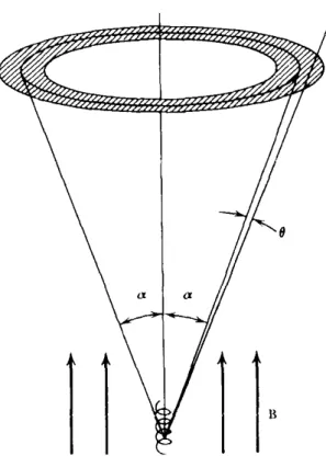
Furthermore, the radiation is concentrated within a small angle around the velocity vector because the particles are moving at high velocities. Thus, a distant observer will sense periodic pulses of radiation as the particle gyrates the magnetic field lines. It can be shown that the period of these pulses is
T ≈ 2π
ω H sin 2 θ (1.8)
where,
θ the paricle’s pitch angle, i.e. the angle between its velocity vector and the magnetic field direction
ω H the relativistic particle gyrofrequency. If the particles are electrons it is given by
ω H = eH
γm e c (1.9)
where m e is the electron mass
Thus, the received power per unit solid angle will be modulated by the fundamental fre- quency, given by the inverse of Eq. 1.8, and its higher harmonics. Using a similar definition to Eq. 1.5, the received power per unit solid angle for an observer located at distance R from the emitting particle and for each of these harmonics, n, is given by
˜
p nΩ = c
2π | E n | 2 R 2 (1.10)
This is larger than Eq. 1.5 by a factor of 2 because both the nth and ( − n)th harmonics of the electric field contribute equally to the power in the nth harmonic, since p ˜ nΩ ∝ E n E ∗ n and E(t) is a real function, i.e. E ∗ n = − E −n (see also Eq. 1.11). We have to take this fact into consideration for our calculations even though negative harmonics have no physical meaning.
In order to evaluate Eq. 1.10, we need an expression for the harmonics of the electric field, E n . First, we estimate the electric field, E(t), of a synchrotron emitting particle by replacing the velocity and acceleration vectors for its helical trajectory in Eq. 1.4 and then we calculate its harmonics, given by the Fourier transform
E n = ω H 2π sin 2 θ
Z
2πsin2θωH