Symmetric Functionals over Tensor Product Spaces in the Context of Quantum Information Theory

Symmetric Functionals over Tensor Product Spaces in the Context of Quantum Information Theory

I n a u g u r a l - D i s s e r t a t i o n

zur

Erlangung des Doktorgrades

der Mathematisch-Naturwissenschaftlichen Fakult¨ at der Universit¨ at zu K¨ oln

vorgelegt von Moritz Fabian Ernst

aus Kleve

Berichterstatter: PD Dr. Rochus Klesse Prof. Dr. Simon Trebst

Tag der letzten m¨ undlichen Pr¨ ufung: 03.12.2014

Kurzzusammenfassung

Die Arbeit besteht im Wesentlichen aus drei Teilen. Wir beginnen unsere Untersu- chung mit einer knappen Einf¨ uhrung in offene Quantensysteme. Daraufhin erkl¨ aren wir verschiedene Maße zur Unterscheidbarkeit von Dichteoperatoren, insbesondere die Uhlmann-Fidelity, welche als Grundlage f¨ ur das in dieser Arbeit studierte Modell dienen wird.

Detaillierter widmen wir uns dann der zeitlichen Entwicklung offener Systeme und f¨ uhren einen wichtigen Begriff der Quanteninformationstheorie ein, den des Quanten- informationskanals. Dieser erm¨ oglicht uns, ein zentrales Problem der Quanteninfor- mationstheorie zu formulieren: Die Bestimmung der Quanteninformationskapazit¨ at eines Quanteninformationskanals. Als wesentliche Schwierigkeit dabei stellt sich das Maximieren der Coherent Information heraus, eine auf dem n-fachen Tensorprodukt eines Hilbertraumes definierte Funktion, die auf Grund ihrer Nichtadditivit¨ at im Li- mes n → ∞ zu betrachten ist.

Um einen Zugang zu diesem derzeit noch ungel¨ osten Problem zu bekommen, studie- ren wir in dieser Arbeit eine ebenfalls auf dem n-fachen Tensorproduktraum definierte Funktion, die Channel-Fidelity eines Quantenkanals. Diese ist ebenfalls nicht additiv und hat somit eine wesentliche Eigenschaft mit der Coherent Information gemein.

Sie ist allerdings im Gegensatz zu dieser mathematisch zug¨ anglicher. Wir fassen die Channel-Fidelity als Modell der Coherent Information auf und studieren ihre Eigen- schaften.

Im zweiten Teil geben wir nach einer kurzen Einf¨ uhrung in die Darstellungstheorie symmetrischer und unit¨ arer Gruppen eine konkrete Anleitung zu Collins’ und ´ Sniadys Formel zur Integration von Funktionen von Matrixelementen unit¨ arer Gruppen ¨ uber das Haar’sche Maß. Schließlich vereinfachen wir diese Formel auf ein f¨ ur die Untersu- chung der Channel-Fidelity optimales Niveau.

Im dritten Teil berechnen wir allgemeine Momente der Channel-Fidelity-Verteilung f¨ ur beliebige n. Um konkretere Ergebnisse zu erzielen beschr¨ anken wir uns auf Pauli- Kan¨ ale. F¨ ur diese diskutieren wir f¨ ur Mittelwert und Varianz den ¨ Ubergang von klei- nen n zum Limes n → ∞ und k¨ onnen f¨ ur beide eine explizite Formel f¨ ur diesen ange- ben. Insbesondere stellt sich heraus, dass f¨ ur eine große Anzahl n von Pauli-Kan¨ alen die Verteilung sehr stark um den Mittelwert konzentriert ist. Weiterhin erm¨ oglicht uns die vereinfachte Formel aus dem zweiten Teil unter gewissen Voraussetzungen die konkrete Berechnung h¨ oherer Momente.

Schließlich vergleichen wir unsere neuen Resultate mit unseren Ergebnissen aus ei-

ner ¨ alteren Arbeit. In dieser hatten wir nach Maxima der Channel-Fidelity gesucht

und haben f¨ ur Pauli-Kan¨ ale Zust¨ ande gefunden, die die Channel-Fidelity zumindest

lokal maximieren. Da diese lokalen Maxima weit oberhalb des Mittelwertes der stark

konzentrierten Verteilung liegen, folgern wir, dass diese mit einem gew¨ ohnlichen Maxi-

mierungsverfahren kaum zu finden sind. Sollte die Channel-Fidelity in dieser Hinsicht

ein gutes Modell f¨ ur die Coherent Information darstellen, stellt deren Maximierung

damit ein sehr schwieriges Problem dar.

Abstract

This thesis consists of three parts. We begin our investigation with a brief introduction into open quantum systems. Then we explain different measures of distinguishability of density operators, especially the Uhlmann Fidelity, which will be the basis for the model function we investigate in this work. We continue by explaining the time evolution of open quantum systems in more detail, and introducing the important notion of quantum channels as a concept in quantum information theory. This allows us to state a central problem of quantum information theory: the characterization of the quantum information capacity of a given quantum channel. The major challenge is the maximization of the coherent information, a function defined on a n-fold tensor product of a Hilbert space, which is non-additive and thus has to be considered in the limit as n → ∞.

To gain an insight into this unsolved problem, we study the channel fidelity of a quantum channel, which is a simpler function, also defined on n-fold tensor pro- duct spaces. It shares an essential feature with the coherent information in being non-additive. However, in contrast to the coherent information it is mathematically accessible. We establish the channel fidelity as a model for the coherent information and study its properties.

In the second part, a short introduction to the representation theory of symmetric and unitary groups is followed by concrete instructions for Collins’ and ´ Sniady’s formula for the integration of functions of matrix elements of unitary groups with respect to the Haar measure. This exposition culminates in a simplification of the general formula that is optimal for investigating the channel fidelity.

In the third part, we calculate channel fidelity moments for arbitrary n. In order to obtain more concrete results, we restrict ourselves to the study of Pauli channels.

For these we discuss the transition of the average and variance from small n to the limit n → ∞ and give an explicit formula for both in this limit. In particular, we find that for a large number n of Pauli channels, the channel fidelity distribution is peaked very strongly. Additionally, under certain restrictions, the simplified formula from part two also allows us to give concrete expressions for higher moments in the limit n → ∞.

We conclude by comparing our new results with results from a former work, where, in

the search for maximizing states of the channel fidelity, we found states that maximize

the channel fidelity of Pauli channels, at least locally. Because these local maxima have

a much higher fidelity than the average of the very strongly peaked distribution, we

infer that these states would not be found by a standard numerical maximization

procedure. If the channel fidelity models the coherent information accurately in this

regard, its maximization thus poses a very hard problem.

Contents

Kurzzusammenfassung iii

Abstract v

1. Introduction 1

1.1. Quantum Information — Open Quantum Systems . . . . 1

1.2. Distinguishing Quantum States . . . . 5

1.2.1. Trace Distance . . . . 6

1.2.2. Uhlmann Fidelity . . . . 7

1.3. Quantum Channel — Completely positive maps . . . . 8

1.4. Unital Qubit Channel . . . . 18

1.5. Channel Capacity: a Challenge in Quantum Information Theory . . . 21

1.5.1. Entropy Exchange . . . . 22

1.5.2. Comparison to Classical Capacity . . . . 24

1.5.3. Subjects for this Thesis . . . . 25

2. Integration over Unitary Groups 27 2.1. Some Group Theory . . . . 28

2.1.1. On Permutations and Cycles . . . . 28

2.1.2. Orbits and Symmetries . . . . 31

2.2. An Introduction to Representation Theory . . . . 34

2.2.1. Schur-Weyl Duality . . . . 37

2.2.2. Young Diagrams: Hooks and Contents . . . . 38

2.2.3. Dimensions . . . . 39

2.2.4. Further characterization of Symmetric Groups . . . . 40

2.2.5. Frobenius Character Formula . . . . 42

2.3. Integrals over Unitary Groups . . . . 44

2.3.1. Illustrative Examples . . . . 44

2.3.2. Sums of Weingarten Functions . . . . 48

2.3.3. Integration over only one row . . . . 49

2.3.4. Cycles and Traces, a First Observation . . . . 50

2.3.5. Q-Correlator . . . . 50

2.3.6. Afterthought: Dimension of a Permutation . . . . 52

3. Channel Fidelity 53 3.1. Motivation . . . . 53

3.2. Average Channel Fidelity for multiple Channels . . . . 54

3.3. Higher Order Moments . . . . 62

3.4. Variances for Generic Quantum Channels . . . . 64

3.4.1. General Symmetry Observations . . . . 65

3.4.2. Symmetry Observations for Self-Adjoint Channels . . . . 69

3.4.3. Variances for Unital Quantum Channels . . . . 70

3.5. Correlations & Diagrams . . . . 78

3.6. Central Moments and Diagrams . . . . 84

3.7. Cumulants in the Limit . . . . 91

3.8. Maximizing Channel Fidelities . . . . 99

3.8.1. An Improved Algorithm? . . . 104

3.8.2. Final Discussion of Channel Fidelity Distribution . . . 105

4. Conclusion 111

A. Estimates for Variance Calculation 113

B. Code 115

C. Tables 121

Acknowledgments 131

Erkl¨ arung 133

1. Introduction

1.1. Quantum Information — Open Quantum Systems

To study quantum information, it is essential to understand the concepts of open quantum systems. We will now begin with the basic notions of quantum mechanics and explain how we can interpret pure state quantum mechanics as the quantum mechanics of closed systems, and how by going over to open quantum systems, the density operator formalism arises naturally. All the following concepts can be found in any advanced quantum mechanics course or an introductory text on quantum computing, for example [26].

The most basic structure of relevance is the Hilbert space of a physical system.

Definition 1.1.1 (Hilbert Space). A complex vector space H ∼ = C

equipped with the standard hermitian inner product is called a Hilbert space. Very often, when we have to consider multiple Hilbert spaces, we will differentiate them with an index H

and denote their normalized basis as {|ii

}

. If there is no confusion possible, sometimes we will drop the index j on the basis.

Typically the inner product of a Hilbert space is denoted in bra-ket notation: For two elements |φi and |ψi in H we write hφ| |ψi, where the left braket means the adjoint vector: hφ| = |φi

.

If we have full knowledge of the system, the system will be in a pure state, which can be described as a vector from the Hilbert space.

Definition 1.1.2 (Pure States). The normalized elements of a Hilbert space (|φi ∈ H) or to be more precise, their induced projectors, |φi hφ|, are called pure states.

More generally however, the state of the system will not be so simple and it has to be described by normalized, self-adjoint positive semi-definite operators on H.

Definition 1.1.3. The set of linear operators from H to itself is denoted by L(H).

Definition 1.1.4 (Density Operator). An operator ρ ∈ L(H) on H is called a density operator iff it is positive semi-definite, ρ ≥ 0; hermitian, ρ = ρ

; and its trace is one, Tr (ρ) = 1.

In agreement with the standard physics notation we usually use single small Greek

letters to denote density operators, e.g. ρ, σ. A density operator will not generally

be a one-dimensional projector.

Fact 1.1.5. A positive semi-definite hermitian operator ρ can be diagonalized as ρ = P

i

p

|ii hi|, for some orthonormal basis, {|ii}

, and positive real numbers {p

}

. If the state of a system is described by a density operator, we usually understand it as a statistical ensemble of systems with isomorphic Hilbert spaces each in a different pure state. The system is in the pure state |ii with probability p

. The p

are a probability distribution over the states.

It is obvious that an arbitrary state cannot be assumed to be pure, but sometimes it can be useful to have a strong contrast to pure states.

Definition 1.1.6 (Mixed State). Let ρ be the density operator of an arbitrary physical system. We call the state of the system mixed iff more than one eigenvalue is larger than zero.

It is a bit surprising that for describing the state of one system we have to think of more than one system. Alternatively, a mixed state can be interpreted as a pure state of a larger system, where the observer restricts herself or himself to only look at a subsystem. The restriction to a subsystem is defined next.

Definition 1.1.7 (Partial Trace). For a combined Hilbert space H

⊗H

and a density operator ρ

on the combined space, we call the mapping

Tr

: L(H

⊗ H

) → L(H

), ρ

7→ ρ

= Tr

(ρ

) = X

i

1

⊗ hi|

(ρ

) 1

⊗ |ii

the partial trace over H

. Alternatively one might say, we trace out H

.

The name partial trace and also the notation suggest that there is a strong connection with the well known notion of a trace. We will now see that the partial trace basically goes halfway towards the trace.

Proposition 1.1.8 (Partial Trace). For a combined Hilbert space H

⊗ H

it is equivalent to trace out H

first and H

second or the other way round. Furthermore, tracing out both systems is equal to the normal trace,

Tr

(Tr

(ρ

)) = Tr

(Tr

(ρ

)) = Tr(ρ

).

Proof. In Definition 1.1.7 we see that:

Tr

(Tr

(ρ

)) = X

j

hj|

X

i

1

⊗ hi|

(ρ

) 1

⊗ |ii

!

|ji

,

which is certainly equivalent to Tr

(Tr

(ρ

)) = X

j

hj|

X

i

hi|

⊗ 1

(ρ

) |ii

⊗ 1

!

|ji

.

Moreover, both expressions can be simplified to:

Tr

(Tr

(ρ

)) = X

i,j

(hj|

⊗ hi|

) (ρ

) (|ji

⊗ |ii

) = Tr (ρ

) .

Using this new tool we can now show that every mixed state can be represented by a pure state of a larger system.

Lemma 1.1.9 (Purification). For ρ = P

i

λ

|ii

hi|

, a positive semi-definite hermi- tian operator on H

= C

, with normalized eigenstates (if necessary, completed to a basis of H

) {|ii

}

, and eigenvalues {λ

}

; and a second Hilbert space H

= C

with d

≥ d

and basis {|ji

}

, there exists a pure state

|φi =

d1

X

i=1

p λ

|ii

⊗ |ii

∈ H

= H

⊗ H

,

where the sum is over all basis vectors of H

and a suitable subset of arbitrary basis vectors of H

such that

Tr

(|φi hφ|) = ρ.

In this way, all states can be purified.

Proof. By tracing out H

:

Tr

(|φi hφ|) = Tr



 X

i,j

p λ

λ

|ii

⊗ |ii

hj|

⊗ hj|





= X

i,j

p λ

λ

|ii

hj|

δ

= X

i

λ

|ii

hi|

In Lemma 1.1.9 we saw that we can choose arbitrary basis vectors of H

for the purification. Thus a purification is not unique.

Lemma 1.1.10. In the same setting as in Lemma 1.1.9, if

|φi = X

i

p λ

|ii

⊗ |ii

∈ H

⊗ H

is a purification of ρ and U

is a unitary transformation on H

, then

|φ

i = X

i

p λ

|ii

⊗ U

|ii

is also a purification of ρ.

Proof. The trace is invariant under cyclic permutations, which extends to partial traces in the obvious way:

Tr

|φ

i hφ

|

= Tr



 X

i,j

p λ

λ

|ii

⊗ U

|ii

hj|

⊗ hj|

U





= Tr



 X

i,j

p λ

λ

|ii

⊗ |ii

hj|

⊗ hj|



 .

Together, Lemma 1.1.9 and Lemma 1.1.10 show that the auxiliary system needs only the same dimension as the system to be purified, since we make no use of a larger space: we can use U

to adjust the order of the basis vectors and then forget about the unused basis vectors.

|φi ∈ H = H

⊗ H

Q

ρ = Tr

(|φi hφ|)

Figure 1.1.: Open Quantum System

In Figure 1.1 we see how we can interpret a mixed state ρ of a system Q as a pure state of a “complete” system where we traced out an environment E about which we do not care. This interpretation is more natural, since we only think of one system.

It is only our lack of knowledge (about the environment) that makes it seem to be an ensemble of systems. The system is open in the sense that there can be hidden interactions with the environment. The implications of this will be discussed in the next section.

Definition 1.1.11 (Open Quantum System). If we know that a quantum system is

in a mixed state, it is an open quantum system and as such, part of a larger, closed

quantum system.

One special quantum system is the smallest non-trivial system — the system on a Hilbert space with dimension two.

Definition 1.1.12 (Qubit). A quantum system where H = C

is called a qubit.

Since a qubit is the smallest non-trivial system, it is central to quantum information theory. We will focus on this system, and especially on its time evolution.

Another useful tool, and also a neat property of tensor products, is the Schmidt decomposition.

Theorem 1.1.13 (Schmidt Decomposition). Let H

and H

be two Hilbert spaces, where dim H

= n and dim H

= m and let n be larger than m.

For an arbitrary |φi ∈ H

⊗H

, there are sets of orthonormal vectors {|1i

, . . . , |mi

} ∈ H

, and {|1i

, . . . , |mi

} ∈ H

, and, up to ordering, a unique set of λ

, . . . , λ

∈ R

, such that

|φi =

m

X

i=1

λ

|ii

⊗ |ii

.

As a result of this section we can — as long as we are not restricted to a specific system — choose to work with pure states. Furthermore, if we need an auxiliary system to purify, it will always be sufficient for the auxiliary system to have the same dimension as the original smaller system.

1.2. Distinguishing Quantum States

For pure states there is a very intuitive and natural way of comparing them: the aforementioned inner product. The inner product is equal to one if and only if the states are equal, and zero only when they are orthogonal. Further, it can be used to compute an overlap of two states, which is the probability to measure the first when the system is actually in the second or vice versa. A high probability indicates that the compared states are close.

In contrast, it is a priori not clear how to find out if two general states ρ

and ρ

are close to each other.

Typically there are only two main concepts [25]. The first, the trace distance, focuses on the operator property, and the second, the fidelity, comes from a more vector- like interpretation of general states. We will use the latter to construct a symmetric functional and analyse the effect of a quantum channel, which will be introduced in the next section, in later parts of this work, Chapter 3.

Before we can get into discussing the two measures, we need to understand that L(H)

is actually a Hilbert space itself. It is quite obvious that the set of linear operators (or

endomorphisms) is a vector space, and we can equip this space with an inner product.

Definition 1.2.1 (Hilbert-Schmidt inner product). Consider two operators A and B on a Hilbert space H. We call

(A, B)

= Tr A

B their Hilbert-Schmidt inner product.

Proposition 1.2.2. The Hilbert-Schmidt inner product is an inner product on the space L(H).

Proof. It is sesquilinear since the trace is linear and taking the adjoint is conjugation for complex numbers. For operators A, B, C and D, and complex numbers λ and µ, we have:

(λA + B, µC + D)

= Tr

λ µ A ¯

C + µ B

C + ¯ λ A

D + B

D

= ¯ λµ (A, C)

+ µ (B, C)

+ ¯ λ (A, D)

+ (B, D)

. It is hermitian:

(A, B)

= Tr

A

B

= Tr (B

A) = (B, A)

. It is positive semi-definite,

(A, A)

= Tr

A

A

≥ 0, since A

A is a positive operator.

As an inner product, it satisfies the Cauchy-Schwarz inequality.

Fact 1.2.3 (Cauchy-Schwarz Inequality).

(ρ

, ρ

)

≤ q

(ρ

, ρ

)

(ρ

, ρ

)

1.2.1. Trace Distance

Equipped with the Hilbert-Schmidt inner product, we can get into exploring the trace distance. First we can generalize the notion of an absolute value to operators.

Definition 1.2.4 (Absolute Value of Operators). Given an arbitrary operator A we call the square root of the inner product with itself its absolute value:

|A| = q

(A, A)

=

√ A

A.

Now the trace distance is defined as the absolute value of the difference of two oper-

ators.

Definition 1.2.5 (Trace Distance). Given two operators A and B, their trace distance D(A, B) is defined as:

D(A, B) = 1

2 Tr (|A − B|) .

The trace distance is a nice measure since it can be used as metric on quantum states ρ. Furthermore, there is a direct physical interpretation.

Example 1.2.6 (Trace Distance). A physical system is prepared in state ρ

with probability

and in state ρ

also with probability

.

ρ

ρ

50%

50%

ρ =?

Figure 1.2.: Distinguishability

A measurement aiming to identify which state has been prepared then has the proba- bility

+

to succeed [25].

1.2.2. Uhlmann Fidelity

The fidelity will be the basis of the symmetric functional that we will investigate extensively in later parts of this thesis. Hence we will take more time to introduce it.

Let us get back to the overlap of two unit vectors.

Example 1.2.7 (Fidelity for Pure States). Take two vectors |φ

i , |φ

i from an arbi- trary Hilbert space H. It is clear that their overlap

F (φ

, φ

) = |hφ

| |φ

i|

is a good way of identifying whether they are identical, F = 1, or orthogonal, F = 0.

The concrete value for F is the probability to measure φ

if the system is in φ

and

vice versa. Furthermore it allows the interpretation of an angle between the two.

Now we seek to extend this functional to general states. On first glance the Hilbert Schmidt inner product seems to be a good candidate. Considering that we are usually interested only in density operators, the inner product of two general states would be 1 only if they are identical and 0 if their supports are mutually orthogonal. However we struggle to interpret the area in between. It is certainly possible to define an angle between two operators using the Hilbert-Schmidt inner product but there is a more natural way:

Definition 1.2.8 (Uhlmann Fidelity). For two operators ρ

and ρ

on H we define their fidelity as the maximal overlap their purifications |φ

i and |φ

i can have:

F (ρ

, ρ

) = max

φ1,φ2

|hφ

| |φ

i|

.

Theorem 1.2.9 (Uhlmann’s Theorem). Maximization is achieved in the following expression:

F (ρ

, ρ

) = Tr q √

ρ

ρ

√ ρ

.

Though it certainly does not look that way, the fidelity is indeed symmetric in its inputs.

The expression in the theorem was considered before by Bures [5], [3], however the interpretation as a transition probability, an overlap between two quantum states, and the proof of equality Theorem 1.2.9 were first done by Uhlmann [35]. The fidelity expression for two general states is quite difficult to handle. Fortunately, comparing a mixed and a pure state is much easier.

Proposition 1.2.10. Let ρ be a mixed state and φ = |φi hφ| be pure. Their fidelity is simply:

F(φ, ρ) = Tr p

|φi hφ| ρ |φi hφ|

= hφ| ρ |φi .

This is why the fidelity is a more natural measure for comparing quantum states. It allows a direct physical interpretation: Imagine an experimenter trying to prepare φ, but he actually prepares ρ. The fidelity describes the probability of success [25].

1.3. Quantum Channel — Completely positive maps

Now we want to transmit quantum information. It is well known that time evolution

in the quantum world is governed by unitary evolution. But this is true only for the

evolution of closed systems. In this section we will first create an intuition about what

we expect a proper quantum channel to be and later describe this mathematically and

give a full characterization. The presented matter is standard material for quantum

information courses and can be found, for example, in [26] or [22].

A quantum channel will describe the time evolution of an open quantum system. We do not make a mistake if we define it as a mapping from one open quantum system (the input) to another quantum system (the output), however, to be a physical map there will additional restrictions and these restrictions will arise naturally in the physical context.

Definition 1.3.1 (Quantum Channel). Consider an input density operator ρ

on the input Hilbert space H

, a quantum channel N and an output Hilbert space H

. A quantum channel is a linear map that maps density operators on H

to density operators on H

:

N : L(H

) → L(H

), ρ

7→ N (ρ

).

Let us now assume we have an open system Q with quantum information ρ

stored in it. We want to understand how the time evolution of the open system Q develops over time.

In quantum mechanics, time evolution of a closed system is described by unitary evolution. An open quantum system is always a part of a larger system. We call the rest of the system the environment E, with density operator ρ

. The process will be influenced by interactions with the E. However the combined system is closed and has the usual unitary time evolution.

⊗

Q E

ρ

ρ

U U ρ

⊗ ρ

U

ρ

= N (ρ

) = Tr

U ρ

⊗ ρ

U

N

Figure 1.3.: Time evolution of an Open Quantum System

Since in the end we only care about the evolution of Q, we trace out E and get the

evolved density operator ρ

. We could easily overlook this as it is obvious that we

want the output ρ

to be a proper density operator, but certainly that is a restriction

on N : it has to preserve the inputs trace and its positivity.

It is a non-essential restriction that input system and output system should always be the same. Sometimes it is too restrictive, for instance in a computation of a precise question the input is often much more complicated then the answer or in an experiment the setup can require a rather large system, where in the end the experimenter only cares about properties of a small part. Let us explore these more general settings in two examples.

⊗

Q E

ρ

ρ

ρ

= N (ρ

) = Tr

U ρ

⊗ ρ

U

N

Figure 1.4.: General Quantum Channel

Example 1.3.2 (Grover’s Algorithm). In Grover’s algorithm [15] the aim is to find a marked state among a set of orthogonal states. As the input the set of states are stored in one system, the function that marks the state in another system. Over the course of the computation other systems might be added, however in the end, the output is only over the system containing the states and an additional qubit indicating if a state is marked or not. We can interpret the action of the algorithm as a quantum channel where input and output systems are inherently different.

Example 1.3.3 (Three Part System). Let us now take a more physical perspective and consider a Hilbert space that is the tensor product of three systems, maybe three qubits, with Hilbert spaces H

, H

, H

.

We can declare any combination of those the input or the output systems. To be clear let us make the example more concrete by choosing H

to be the input system Q with Hilbert space H

thus the environment E with Hilbert space H

= H

⊗ H

and the output P with Hilbert space H

= H

⊗ H

which makes the new environment H

= H

.

As an overview, and because we will have a similar structure when we construct a

quantum channel precisely, we give a list of the different combinations of the three

Hilbert spaces:

H = H

⊗ H

⊗ H

H

= H

H

= H

⊗ H

H

= H

⊗ H

H

= H

H = H

⊗ H

, and H = H

⊗ H

.

Each of these combinations can be a valid interpretation of H. Certainly there are even more complicated tensor product structures possible. By tracing out E

we map quantum information from system Q to system P, as illustrated in Figure 1.4.

In the examples, we have seen that a general quantum channel demands the possibility to send quantum information from one system to another system. We will see that this is not just possible but arises naturally in the physical construction.

Before we get into the mathematical characterization of a quantum channel, we expect another general property: physical extensibility.

Definition 1.3.4 (Extensibility). Consider a Hilbert space that is a tensor product H = H

⊗ H

and a quantum channel N

that is defined for density operators on H

and another quantum channel N

that is defined for density operators on H

. If for all H

and N (A) the combined quantum channel N

⊗ N

is still a proper quantum channel, in the sense that it maps a density operator ρ on H to a valid density operator N

⊗ N

(ρ) on H, N

is called extensible.

ρ

A

⊗ Q

N

⊗ N

N

⊗ N

(ρ)

N

N

Figure 1.5.: Extensibility

Note that the combined system H

⊗ H

is in general still an open quantum system.

We require extensibility, because we want to be free in combining quantum channel with each other without any further restriction. To understand why extensibility is an issue we should formalize our thoughts.

We already mentioned that the essential properties of a density operator, that they are semi definite positive operators with trace one, have to be preserved. It follows that the set of quantum channels is clearly not equivalent to the set of linear maps of operators to operators. We will now see that extensibility shrinks the set further.

Example 1.3.5. For operators on C

consider the transposition map T .

T : L( C

) → L( C

), A 7→ A

,

which clearly is trace preserving and also positivity preserving since A and A

have the same eigenvalues.

Now we extend the map trivially — the trivial map is obviously positivity and trace preserving:

1 ⊗ T : L(C

) ⊗ L(C

) → L(C

) ⊗ L(C

), A 7→ 1 ⊗ T (A).

Now we take a positive semi-definite operator that is not normalized, which makes things easier to read.

A =

















1 0 0 1 0 0 0 0 0 0 0 0 1 0 0 1

















=



 1 0 0 0



 ⊗



 1 0 0 0



 +



 0 1 0 0



 ⊗



 0 1 0 0





+



 0 0 1 0



 ⊗



 0 0 1 0



 +



 0 0 0 1



 ⊗



 0 0 0 1





Apply the extended maps:

1 ⊗ T (A) =



 1 0 0 0



 ⊗



 1 0 0 0



 +



 0 1 0 0



 ⊗



 0 0 1 0





+



 0 0 1 0



 ⊗



 0 1 0 0



 +



 0 0 0 1



 ⊗



 0 0 0 1





=

















1 0 0 0 0 0 1 0 0 1 0 0 0 0 0 1















 ,

and get an operator that has negative determinant:

det ( 1 ⊗ T (A)) = −1.

Thus we see that the extended map is not positivity preserving.

We need to distinguish maps that will, even with extension, preserve positivity, from those that do not. This concept is called complete positivity.

Definition 1.3.6 (Complete Positivity). Consider L(H) for H and an auxiliary sys- tem of arbitrary size H

. A map N is called completely positive if it not only maps positive (semi-definite) maps to positive (semi-definite) maps but also all extensions of N as 1

⊗ N conserve positivity.

The next proposition follows immediately.

Proposition 1.3.7. Complete positivity is necessary and sufficient for physical ex- tensibility.

Proof. The necessity is obvious. For the sufficiency consider four systems H

, H

, H

and H

and two quantum channel N

and N

with:

N

: L(H

) → L(H

), and N

: L(H

) → L(H

).

Then the combined map N

⊗ N

,

N

⊗ N

: L(H

⊗ H

) → L(H

⊗ H

),

is positivity preserving, since we can write the map as a composition of completely positive maps:

N

⊗ N

= (N

⊗ 1

) ◦ ( 1

⊗ N

) = ( 1

⊗ N

) ◦ (N

⊗ 1

) .

The input and output systems are not necessarily equivalent. We have to be careful

that the tensors actually act on the correct spaces.

We have seen that a realistic physical quantum channel has to meet certain require- ments which we conclude in the next proposition.

Proposition 1.3.8. A quantum channel N is trace preserving and completely posi- tive.

We will get a handy standard form for quantum channels once we have a more detailed look at the construction.

As in Figure 1.4, consider a system Q in state ρ

and an environment E in a pure state Φ = |φi hφ|. We can assume the environment to be in a pure state because otherwise it could easily be purified. Furthermore, keep in mind that we have an underlying structure as in Example 1.3.3.

The full input density operator is given by:

ρ = ρ

⊗ Φ.

We want to trace out an arbitrary environment E

of the whole system.

N (ρ

) =

dimE⁰

X

i=1

1

⊗ hi|

U

ρ

Q,E

⊗ φ

U

1

⊗ |ii

Note that the tensor products are not necessarily combining the same spaces as indi- cated by the superscripts.

Now we use that the environment is in a pure state.

N (ρ

) =

dimE⁰

X

i=1

1

P,E⁰

⊗ hi| U

ρ

Q,E

⊗ |φi hφ|

U

1

⊗ |ii

=

dimE⁰

X

i=1

1

P,E⁰

⊗ hi| U

1

Q,E

⊗ |φi

ρ

1

Q,E

⊗ hφ|

U

1

⊗ |ii

The second step looks a bit surprising. This is a weakness of the bra-ket notation.

We are tempted to naively write a 1 beside ρ

. We can clear the mess up by precisely looking at the mappings.

Consider:

ρ

⊗ |φi hφ| : H

⊗ H

→ H

⊗ H

, and ρ

: H

→ H

,

and define:

W

:= 1

Q,E

⊗ |φi : H

→ H

⊗ H

and W

:= 1

Q,E

⊗ hφ| : H

⊗ H

→ H

.

We see that only W

ρ

W

= ρ

⊗ |φi hφ| is well defined.

A hypothetical W

ρ

⊗ 1

W

=? would not make sense.

Finally we define the operators:

A

=

1

⊗ hi|

U W

, (1.1)

which simplifies the quantum channel to:

N (ρ

) =

dimE⁰

X

i=1

A

ρ

A

.

The latter is called the Kraus representation or operator sum representation of a quantum channel.

Definition 1.3.9 (Kraus Representation). A completely positive map N has a Kraus representation or is in Kraus form, if there exist operators A

such that:

N (ρ) = X

i

A

ρA

.

The A

are called Kraus operators.

Theorem 1.3.10 (Quantum Channel). For a completely positive map N the existence of a Kraus form is necessary and sufficient. The map N with Kraus operators A

is also trace preserving iff

X

i

A

A

= 1 .

A proof for this theorem can be found in [21, 7].

It is easy to show that the quantum channel we constructed, is trace preserving.

Proposition 1.3.11. For Kraus operators defined as in Equation 1.1 we have:

X

i

A

A

= 1

and furthermore

Tr (N (ρ

)) = Tr X

i

A

ρ

A

!

= Tr (ρ

).

Proof. The trick is basically to pull the sum through, so that |ii hi| acts as an identity map:

X

i

A

A

= X

i

1

Q,E

⊗ hφ|

U

1

P,E⁰

⊗ |ii 1

⊗ hi|

U

1

Q,E

⊗ |φi

=

1

Q,E

⊗ hφ|

U

X

i

1

P,E⁰

⊗ |ii hi|

U

1

Q,E

⊗ |φi

=

1

Q,E

⊗ hφ|

U

U

1

Q,E

⊗ |φi

= 1

.

Then using the cyclic invariance and linearity of the trace, the second statement follows quickly:

Tr (N (ρ

)) = Tr



 X

i=1,dimE⁰

A

ρ

A



 = X

i=1,dimE⁰

Tr

A

A

ρ

= Tr (1

ρ

) = Tr (ρ

) .

In the next section we will introduce a class of quantum channel that will be relevant in later parts of this work. For now we want to give a few examples.

Example 1.3.12 (Amplitude-Damping Channel [26]). A very intuitive interaction with the environment is energy leakage. One system which we can model is the emis- sion of a photon [26]. Consider a two-dimensional Hilbert space H = C

and the sys- tem in the pure state of a superposition of none and a single photon: |φi = a |0i+b |1i.

The density operator in the |0i,|1i basis is then:

ρ = |φi hφ| =



 a¯ a a ¯ b b¯ a b ¯ b



 .

The amplitude damping channel N

has Kraus operators

A

=





1 0

0 √

1 − γ



 and A

=





0 √

γ

0 0



 ,

which describe a process that lowers the probability of the system to be in state |1i, as

it transports the system to N

(ρ) =





a¯ a a ¯ b √ 1 − γ b¯ a √

1 − γ b ¯ b(1 − γ)



 +



 b ¯ bγ 0

0 0



 =





a¯ a + γb ¯ b a ¯ b √ 1 − γ b¯ a √

1 − γ b ¯ b(1 − γ )



 .

We see that the probability to be in the zero photon state is increased by γ |b|

. We can think of γ as the probability of leaking a photon to the environment.

Note that for γ = 1 we get, for arbitrary input density operators, the pure output state

|0i h0|.

Example 1.3.13 (Von-Neumann Measurement [26]). Consider a system Q in state ρ

. We will now explain how a measurement of this state can be interpreted as a quantum operation N

.

An observable O has to be the weighted sum of projection operators P

, where the P

are mutually orthogonal projectors i.e. O is a self-adjoint operator:

O = X

m

o

P

.

According to Born’s rule, an outcome o

is measured with probability p

: p

= Tr (P

ρ

) .

The measured state ρ

of the system is then:

ρ

= P

ρ

P

p

.

Effectively we can see the measurement process as the mapping with the projectors as Kraus operators:

N

(ρ

) = X

m

p

P

ρ

P

p

= X

m

P

ρ

P

.

Note that since the P

are projectors they are self-adjoint, square to themselves and sum up to the identity:

X

m

P

P

= X

m

P

P

= X

m

P

= 1 ,

and hence fulfill the requirements of for a quantum channel.

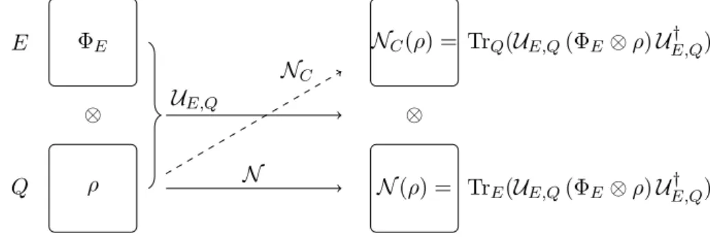
Definition 1.3.14 (Complementary Channel [14, 36]). We have seen that a quantum channel can be interpreted as unitary time evolution of a system Q and a suitable environment E, where the environment’s degrees of freedom are traced out. We can exchange the interpretation of Q and E for the output and construct a map from the operators on Q to the operators on E by tracing out Q instead of E. This map is certainly closely related to N and is called the complementary channel N

.

Q ρ

⊗ ⊗

E Φ

U

N N

Tr

(U

(Φ

⊗ ρ) U

) N (ρ) =

Tr

(U

(Φ

⊗ ρ) U

) N

(ρ) =

Figure 1.6.: Complementary Channel

The complementary channel is essentially unique [24].

Example 1.3.15 (Degradable Channel [14, 36, 24]). An interesting class of channels are those that can be degraded to their complementary channel. That means, that there is another quantum channel N ˜ such that

N

(ρ) = ˜ N (N (ρ)).

Q ρ N

N

N ˜

N (ρ) N ˜ (N (ρ)) N

(ρ) =

If the complementary channel is degradable, N is called anti-degradable.

1.4. Unital Qubit Channel

In our characterization of quantum channels, we ignored that we actually have the

freedom to choose the bases for input and output system. Let us consider now that in

an experimental setting we have a quantum channel with Kraus operators A

. Then at the input side we can choose a specific input basis by using a unitary operator W and also on the output side a specific output basis by applying a unitary operator V . This will allow us to transform the channel:

N (ρ) = X

i

A

ρA

7→ N

(ρ) = X

i

V A

W ρW

A

V

= X

i

A

ρA

.

The channels N and N

are closely related, since their outputs are unitarily similar.

Still the freedom to choose input and output bases can come in handy for specific channels. A very nice example is the unital qubit channel.

Definition 1.4.1. A quantum channel N is called unital iff it maps the identity of the input system to the identity of the output system, i.e.

N ( 1 ) = X

i

A

1 A

= 1 .

Corollary 1.4.2. The adjoint map N

of a unital channel N is also trace preserving and therefore a quantum channel.

Proof. Let {A

}

be the Kraus operators of N . Then the Kraus operators of N

are by definition B

≡ A

. Furthermore, since N is unital we have:

1 = X

i

A

1 A

= X

i

B

B

.

Theorem 1.4.3 (Pauli Channel). For unital qubit channel N , where dim Q = 2, there exists a canonical form [2], N

i}³_i=0

: N

i}³_i=0

(ρ) =

3

X

i=0

p

σ

ρσ

, X

i

p

= 1,

with the Pauli operators σ

and the identity σ

= 1

. The standard Kraus form can be obtained with A

= √

p

σ

. A unital qubit channel that is in canonical form is called a Pauli channel, N

i}³_i=0

, with probabilities, {p

}.

The proof is rather involved, and furthermore the simple structure is special for d = 2.

Unital channels in higher dimension can still be written as an affine combination of unitaries, however these do not have the nice structure that only one operator has a trace different to 0 [23, 10].

We will focus on qubit channels. Whenever we have the choice of input and output

bases we will use the canonical form.

One special Pauli channel that is easy to understand is the bit flip channel. It has only one parameter. We will sometimes use it for plots.

Example 1.4.4 (Bit Flip Channel). We call the Pauli channel where p

= p

= 0, p

= p and p

= (1 − p) the bit flip channel N

, as it flips the bit with probability (1 − p).

However, since the bit flip channel is degradable, [14], it is already well understood.

We will see what this means in the next section.

Depolarizing Channel

As we want to plot functionals that depend on error probabilities, it will be useful to only have a single parameter. A special quantum channel with this property is the depolarizing channel N

. It maps an input state to a linear combination of the input and the maximally mixed state.

Definition 1.4.5 (Depolarizing Channel). The depolarizing channel is defined by the action:

N

(ρ) = λρ + 1 − λ d 1

.

It is non-trivial but well known [26, 3] that for d = 2, the depolarizing channel can be written as a Pauli channel.

Proposition 1.4.6 (Depolarizing Channel). The depolarizing channel as a Pauli channel with parameter p is given by:

N

(ρ) = N

3 ,^1−p₃ ,^1−p₃ }

(ρ) = p σ

ρσ

+ (1 − p) 3

3

X

i=1

σ

ρσ

.

We will prefer the interpretation as a Pauli channel, since most of our results apply only to such channels. The depolarizing channel is not degradable, which makes it more interesting to study than the bit flip channel.

A special case of the depolarizing channel is the channel that maps all inputs to the completely mixed state, which is equivalent to λ = 0 in Definition 1.4.5.

Definition 1.4.7 (Completely Depolarizing Channel). The completely depolarizing channel is the depolarization channel with λ = 0, which can be expressed as a Pauli channel as:

N

(ρ) =

3

X

i=0

1

4 σ

ρσ

= 1

2 .

1.5. Channel Capacity: a Challenge in Quantum Information Theory

Now that we have introduced the notion of quantum information transmission the next logical step is to characterize it.

The name quantum channel directly suggests that it will be used to send quantum information and thus it is a an obvious question, how much information can be reliably transmitted.

Definition 1.5.1 (Quantum Capacity of a Quantum Channel). The quantum capac- ity Q(N ) of a quantum channel N is its ability to transmit quantum information. It is measured in qubits per channel use.

This question has been partially answered by the quantum Shannon theorem.

Theorem 1.5.2 (Quantum Shannon). For a quantum channel N its quantum capac- ity is the maximal regularized coherent information in the limit of n → ∞ channel,

Q(N ) = lim

n→∞

I

(N ).

The proof for this theorem is rather involved [17, 19] and we will not present it here, however we will try to create an intuition for it and in the end compare it to the classical capacity of a classical channel.

In some sense information that is stored in a system is the opposite of the uncertainty about the system. Therefore its information content can be measured by its von- Neumann entropy.

Definition 1.5.3 (Von-Neumann Entropy). For a density operator ρ the von-Neumann entropy S(ρ) is given by:

S(ρ) = −Tr (ρ log

ρ) .

With this measure of information, we can define a measure for the information a quantum channel can transport, the coherent information.

Definition 1.5.4 (Coherent Information). For quantum information stored in a den- sity operator ρ and a quantum channel N that can transport ρ we define their coherent information I (ρ, N ) as:

I(ρ, N ) = S(N (ρ)) − S

(ρ, N ).

The coherent information is the information of the output S(N (ρ)) minus the in- formation lost to the environment S

(ρ, N ), called the entropy exchange, and to be defined shortly. Before we get into explaining the latter, we have to understand that in the quantum world entanglement effects can occur, and these make it possible that multiple copies of the same channel can actually transport more information per channel than a single channel, [9, 28, 13], thus we have to consider the coherent information for n channels, but per channel.

Definition 1.5.5 (Regularized Coherent Information).

I

(N ) = 1 n max

ρ

I(ρ, N

)

If the regularized coherent information is equal to the coherent information, the ca- pacity can be calculated easily. This is the case for example for degradable channels, [13], [36]. This is why the bit flip channel, Example 1.4.4, is not at the center of our attention, whereas the depolarizing channel, Proposition 1.4.6, is.

However if the regularized coherent information is not equal to the coherent infor- mation, we can understand why the question is only partially answered. Since the dimension of H or ρ for that matter grows exponentially with the number of channels, a maximization for only n = 10 would already be very difficult and that is not even close to a limit of n → ∞.

Ideally one would find an explicit n-dependent expression for I

, such that one can analytically maximize it and then take the limit of n → ∞. These expressions are called single letter formulas.

Definition 1.5.6 (Single Letter Formula). For a functional F over a Hilbert space that can naturally be extended to a tensor product of n Hilbert spaces, an explicit, n-dependent expression is called a single letter formula.

1.5.1. Entropy Exchange

We will now motivate the concept of entropy exchange, S

(ρ, N ).

The following small proposition is essential.

Proposition 1.5.7 (Entropy of Partial Traces). Consider two density operators ρ

on H

and ρ

on H

that can be purified to the same state Ψ = |ψi hψ|:

Tr

(Ψ) = ρ

, and Tr

(Ψ) = ρ

. Then ρ

and ρ

have the same entropy.

Proof. Since |ψi ∈ H

⊗ H

is a state from a product space, it has a Schmidt decom- position, Theorem 1.1.13, |ψi = P

i

√ p

|ii ⊗ |ii, which makes it easy to calculate:

S(ρ

) = S(ρ

) = X

i

p

log

(p

).

We will now see that a quantum channel can lose information to the environment; it can exchange information between the open system and the environment.

Definition 1.5.8 (Entropy Exchange). Consider a quantum system Q with environ- ment E and an auxiliary space R such that an operator ρ on H

can be purified to a state Ψ

= |ψi hψ| with |ψi ∈ H

⊗ H

. Furthermore N shall be a quantum channel with unitary evolution over H

⊗ H

. The entropy exchange S

between Q and E is given by:

S

(ρ, N ) = S ([ 1

⊗ N ] (Ψ

)) . We will explain this definition further in the following example.

Example 1.5.9 (Entropy Exchange). Consider a situation as in the above definition or the following picture.

⊗

⊗ E

Q

R Φ

ρ

U

N

1

⊗ ⊗

⊗

Ψ

ρ

ρ

Figure 1.7.: Entropy Exchange

Quantum information ρ is stored in system Q. ρ is purified to Ψ

using the auxiliary system R. A quantum channel N describes a time evolution of ρ with an underlying unitary interaction U

between Q and an environment E. In the beginning the state of the environment is the pure state Φ

. Since the auxiliary system R is not involved in the unitary interaction its time evolution is given as the identity 1

. Considering all of this, the full input state is ρ

= Φ

⊗ Ψ

and the full time evolution can be written in the following way:

[U

⊗ 1

] (ρ

) = ρ

.

Note that both ρ

and ρ

are pure states and thus their entropies are zero.

The same is true for the environment alone.

Now we take the partial trace to get output operators for E and Q ⊗ R alone:

ρ

= Tr

(ρ

),

ρ

= Tr

(ρ

) = [ 1

⊗ N ] (Ψ

) .

These are in general mixed states with the same entropy Proposition 1.5.7: This means that the entropy of E has changed from zero to a finite value. This explains the name entropy exchange: Entropy has been exchanged between the combined system Q ⊗ R and the environment E.

1.5.2. Comparison to Classical Capacity The following is based on Shannon’s original paper, [27].

The information content of a random variable is measured by its Shannon entropy.

Definition 1.5.10 (Shannon Entropy). For a random variable X with possible values x

, . . . , x

and their probabilities p(x

), its Shannon Entropy is

H(X) = −

n

X

i=1

p(x

) log

(p(x

)).

Since we seek to compare two random variables, namely the output of a channel given a certain input, we need the concept of conditional entropy.

Definition 1.5.11 (Conditional Entropy). For two random variables X with possible values x

, . . . , x

and their probabilities p(x

) and Y with possible values y

, . . . , y

and their probabilities p(y

) as in Definition 1.5.10 the conditional entropy of Y given X is

H(Y |X) =

n

X

i=1

p(x

)H(Y |X = x) = −

n

X

i=1 m

X

j=1

p(x

, y

) log

p(x

, y

) p(x

)

.

With this tool we can describe how much two probability distributions have in com- mon.

Definition 1.5.12 (Mutual Information). For two random variables X and Y their mutual information is given by:

I (X, Y ) = H(Y ) − H(Y |X).

Similar to the coherent information, Definition 1.5.4, the mutual information is the information content of the output minus a relation between output and input.

It is, however, rather difficult to completely motivate these statistical measures. Mu- tual information and coherent information as concepts have to show and have shown their usefulness in the characterization of (quantum) information transmission [1] and especially (quantum) channel capacities.

The validity of mutual information has been shown by [27], as it provides a formula

to obtain the capacity of a classical channel.

Theorem 1.5.13 (Shannon). For a classical channel N that maps a random variable X to another random variable N (X), its classical capacity C(N ) is the maximum over all possible inputs,

C(N ) = max

X

I (X, N (X)).

On first glance the two capacities look very similar, especially because they character- ize the capacity of a channel as the capacity for an optimal input. The big difference is that for a feasible input system, the classical capacity can easily be computed nu- merically, whereas the quantum capacity is much more difficult to handle; even a small input system leads to an unsolvable optimization problem over a vast space.

1.5.3. Subjects for this Thesis

Finding the general capacity of a quantum channel, especially for most Pauli channels, is still an open question. Ultimately we are interested in a solution to this problem, however we do not have a direct approach and will be content with studying the effect of high tensor powers of quantum channels more generally.

We will investigate a quantity, the channel fidelity, that is much simpler than the coherent information, in the sense that it is much easier to handle mathematically, however complicated enough such that it will show entanglement dependence. For us the channel fidelity only allows pure inputs to a quantum channel and then compares this input to the output of the quantum channel. A more precise definition will be found in the beginning of Chapter 3.

We begin our investigation by computing moments of the channel fidelity distribution, in particular the average and the variance. We will even find single letter formulas (see Definition 1.5.6) for these. This will allow us to study the effect of multiple quantum channels on the channel fidelity distribution. Later, we analyze the structures that lead to single letter formulas. After explaining the structures we can use them to find single letter formulas for higher moments, under certain restrictions. In the end we will compare our insights about the distribution with results of previous work, where we used an iterative algorithm to find maximizing states.

For the moment calculation we will need additional mathematical tools. We will

introduce these in Chapter 2.