The Relation between Divorce and Wealth
Dissertation zur Erlangung des akademischen Grades eines doctor rerum politicarum (Dr. rer. pol.)
an der Fakultät Sozial- und Wirtschaftswissenschaften der Otto-Friedrich-Universität Bamberg
vorgelegt von
Dipl.-Volksw. Anna Fräßdorf
Erstgutachter: Prof. Dr. Frank Westerhoff Zweitgutachter: Prof. Dr. C. Katharina Spieß Tag der mündlichen Prüfung: 13.07.2011
Danksagung
An dieser Stelle möchte ich den Personen danken, die mich bei der Umsetzung dieser Arbeit unterstützt haben. Mein Dank gilt vor allem meinem Doktorvater Johannes Schwarze für seine tatkräftige Unterstützung im Laufe der letzten Jahre. Seine Bereitschaft, neue Ideen zu diskutieren, und seine konstruktive Kritik haben die Entstehung der Arbeit stets gefördert. Des Weiteren danke ich Frank Westerhoff, dass er sich nach Johannes Schwarzes Tod bereit erklärt hat, das Erstgutachten meiner Dissertation zu übernehmen. Auch Katharina Spieß möchte ich dafür danken, dass sie mich weiter unterstützt hat.
Meine Arbeit profitierte von Diskussionen auf verschiedenen internationalen Konferenzen sowie dem regen Austausch mit Mitarbeitern und Doktoranden des DIW Berlin. Vor allem Markus Grabka bin ich für seine Unterstützung zu Dank verpflichtet. Den Mitarbeitern des RatSWD danke ich dafür, dass sie mich so herzlich bei sich aufgenommen haben. Außerdem gilt mein Dank Monika Sander und allen Mitarbeitern des Lehrstuhls für Empirische Mikroökonomik, die meine Arbeit durch ihre Kommentare und Vorschläge unterstützt haben. Bei der DFG möchte ich mich für die finanzielle Förderung im Rahmen des Graduiertenkollegs
„Märkte und Sozialräume in Europa“ bedanken.
Meinen Eltern, meinen Freunden und Mathis bin ich sehr dankbar für ihre liebevolle Unterstützung in allen Lebenslagen. Ich danke ihnen für ihr Vertrauen, ihren moralischen Beistand und das Interesse an meiner Arbeit.
Table of Content
List of Figures ... 1
List of Tables ... 2
List of Acronyms ... 5
Executive Summary ... 7
Introduction ... 10
1 Theoretical Background ... 18
2 2.1 Economic Theory of Marriage ... 18
2.2 Legal Regulation of Marriage and Divorce ... 26
2.3 The Concept of Wealth ... 30
2.4 Wealth Accumulation ... 35
2.5 Wealth and Marital Status ... 38
2.6 Literature Review ... 47
2.6.1 The Distribution of Wealth ... 47
2.6.2 Marital Splits and Wealth ... 49
Data and Methods ... 54
3 3.1 Data ... 54
3.1.1 Wealth Data in the SOEP ... 54
3.1.2 Editing and Imputation to Account for (Non-) Sampling Errors ... 56
3.1.3 Martial Histories in the SOEP ... 60
3.2 Methods ... 65
3.2.1 The Problem of Endogeneity ... 65
3.2.2 Instrumental Variable Approach ... 67
3.2.3 Quasi-experimental research design ... 71
3.2.4 Matching ... 71
3.2.5 Conditional Difference-in-Differences Matching ... 81
3.3 Dependent and Explanatory Variables ... 84
Empirical Evidence ... 96
4 4.1 The Distribution of Wealth ... 96
4.2 The Distribution of Wealth by Marital History ... 103
4.3 The Distribution of Wealth by Marital Changes ... 115
4.4 Assessing the Causal Effect of Divorce on Wealth ... 124
5 Summary ... 130 References ... 133 6
Appendix ... 151 7
1
List of Figures
Figure 1: Number of divorces and marriages in Germany 1960-2008 ... 15
Figure2: The formation of personal wealth ... 32
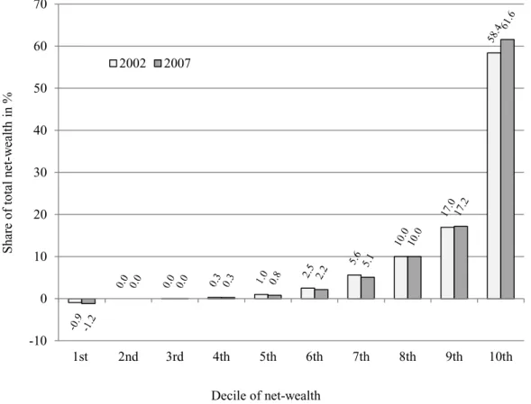
Figure 3: Percentage share of net-wealth over deciles in 2002 and 2007. ... 97
Figure 4: Net-wealth in 2002 and 2007 by marital status changes categories ... 116
Figure 5: Net-wealth in 2002 and 2007 by marital status changes categories and gender ... 118
Figure A 1: SOEP person questionnaire 2002 – balance sheet ... 151
Figure A 2: SOEP person questionnaire 2007 – balance sheet ... 153
Figure A 3: SOEP person biography – retrospective recording of family status ... 155
Figure A 4: Changes in family situation ... 155
Figure A 5: Current marital status ... 155
Figure A 6: Mean of net-wealth 2002 and 2007 by age class ... 156
2
List of Tables
Table 1: Numeric example “Zugewinnausgleich” ... 29
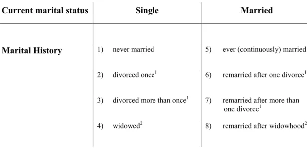
Table 2: Marital status categories ... 63
Table 3: Categories of marital changes ... 65
Table 4: Counterfactual inference ... 72
Table 5: Overview of dependent and control variables for OLS regressions and (ordered) probit regression models ... 91
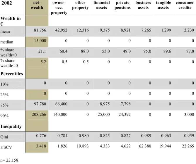
Table 6: The distribution of wealth in 2002 ... 98
Table 7: The distribution of wealth in 2007 ... 99
Table 8: The distribution of wealth by gender 2002 ... 101
Table 9: The distribution of wealth by gender 2007 ... 102
Table 10: The distribution of wealth by marital history 2002 ... 104
Table 11: The distribution of wealth by marital history 2007 ... 105
Table 12: The distribution of wealth by marital history and gender 2002 ... 107
Table 13: The distribution of wealth by marital history and gender 2007 ... 109
Table 14: Coefficients for marital status ... 113
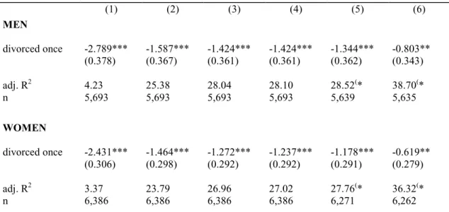
Table 15: Coefficients for the “divorced once” category ... 114
Table 16: Coefficients for marital status changes between 2002 and 2007 ... 119
Table 17: Coefficients for the “divorced once” category ... 121
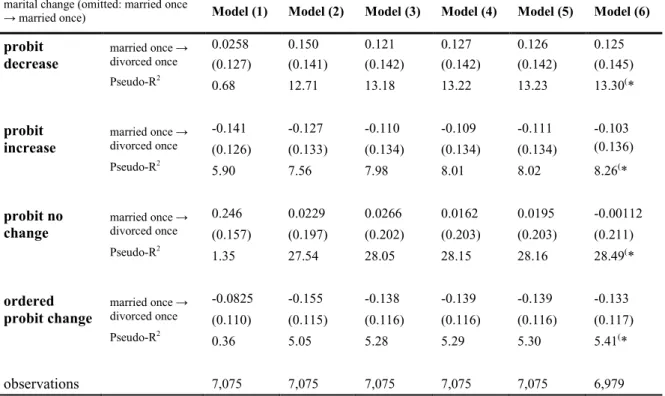
Table 18: Results of (ordered) probit regressions on the change in wealth for men 122 Table 19: Results of (ordered) probit regressions on the change in wealth for women ... 123
Table 20: Results of conditional difference-in-differences matching for men ... 128
Table 21: Results of conditional difference-in-differences matching for women ... 129
Table A 1: Coefficients of OLS regression on IHS-transformed net-wealth 2007 for men ... 157
Table A 2: Coefficients of OLS regression on IHS-transformed net-wealth 2007 for women ... 160
Table A 3: Coefficients of OLS regression on the change in IHS-transformed net- wealth between 2002 and 2007 for men ... 163
3 Table A 4: Coefficients of OLS regression on the change in IHS-transformed net- wealth between 2002 and 2007 for women ... 168 Table A 5: Coefficients of probit regression on whether net-wealth increased by more than 5% between 2002 and 2007 for men ... 173 Table A 6: Coefficients of probit regression on whether net-wealth increased by more than 5% between 2002 and 2007 for women ... 178 Table A 7: Coefficients of probit regression on whether net-wealth decreased by more than 5% between 2002 and 2007 for men ... 183 Table A 8: Coefficients of probit regression on whether net-wealth decreased by more than 5% between 2002 and 2007 for women ... 188 Table A 9: Coefficients of probit regression on whether the change in net-wealth between 2002 and 2007 did not exceed a 5% decrease or increase for men ... 193 Table A 10: Coefficients of probit regression on whether the change in net-wealth between 2002 and 2007 did not exceed a 5% decrease or increase for women ... 198 Table A 11: Coefficients of ordered probit regression on the change in net-wealth between 2002 and 2007 for men ... 203 Table A 12: Coefficients of ordered probit regression on the change in net-wealth between 2002 and 2007 for women ... 208 Table A 13: Distribution of control variables for the OLS regression on IHS- transformed net-wealth in 2007 ... 213 Table A 14: Distribution of control variables for the OLS regression on the change in IHS-transformed net-wealth between 2002 and 2007 ... 216 Table A 15: Calculation of the propensity scores ... 221 Table A 16: Balancing tests for 10 nearest neighbours within a 0.05 caliper for men ... 223 Table A 17: Balancing test for 10 nearest neighbours within a 0.05 caliper for women ... 225 Table A 18: Balancing tests for 5 nearest neighbours within a 0.05 caliper for men ... 227 Table A 19: Balancing test for 5 nearest neighbours within a 0.05 caliper for women ... 229 Table A 20: Balancing tests for 1 nearest neighbour within a 0.05 caliper for men 231
4 Table A 21: Balancing test for 1 nearest neighbour within a 0.05 caliper for women
... 233
Table A 22: Balancing test for kernel matching (bandwidth 0.01) for men ... 235
Table A 23: Balancing test for kernel matching (bandwidth 0.01) for women ... 237
Table A 24: Balancing test for local linear matching (bandwidth 0.01) for men... 239 Table A 25: Balancing test for local linear matching (bandwidth 0.01) for women 241
5
List of Acronyms
ATE Average Treatment Effect
ATT Average Treatment Effect of the Treated
BGB Bürgerliches Gesetzbuch
CIA Conditional Independence Assumption CMIA Conditional Mean Independence Assumption
CPS Current Population Survey
DJI Deutsches Jugendinstitut
EheRG Ehereformgesetz
EVS Einkommens- und Verbrauchsstichprobe
FDZ-RV Forschungsdatenzentrum der Rentenversicherung
HINK Swedish Household Income Survey
HRS Health and Retirement Study
HSCV Half the Squared Coefficient of Variation IHS Inverse Hyperbolic Sine-Transformation
ISCED International Standard Classification of Education
IV Instrumental Variable
LWS Luxembourg Wealth Study
NLS National Longitudinal Survey
NLSY79 National Longitudinal Survey of Youth 1979
OECD Organisation for Economic Co-Operation and Development
OLS Ordinary Least Squares
PSID Panel Study of Income Dynamics
PSM Propensity Score Matching
RCM Rubin Causal Model
SCF Survey of Consumer Finances
6
SOEP Socio-Economic Panel
SUTVA Stable Unit Treatment Value Assumption
7
Executive Summary
Wealth is a crucial parameter for economic well-being and fulfils several functions.
It generates direct financial income such as capital gains, constitutes a source of consumption as well as a buffer during spells of economic stress and thus provides economic security, for instance. Wealth is of high importance with regard to intergenerational transfers and bequests which have a share in maintaining existing inequalities. Furthermore, the importance of wealth holdings accumulated for retirement purposes has increased in recent years. Despite of the particular importance of wealth as a measure of economic well-being and the various functions of wealth, its distribution on the individual level as well as the reasons for inequality in wealth holdings in Germany have not been fully explored.
Amongst other things, current wealth holdings are determined by previous wealth, (permanent) income and consumption, and hence by saving. Shocks with regard to these determinants, e.g. unemployment or sickness, can affect wealth holdings.
Marital splits constitute another potential shock in relation to wealth. Divorce is likely to reduce wealth holdings directly, as court and lawyer fees are incurred by divorces. Additionally, divorce is related to wealth indirectly, since family status correlates with the determinants of wealth. Marital splits can reduce (permanent) income in consequence of ceasing eligibility for fiscal privileges or the loss of specialisation gains. Consumption needs may be relatively lower for a couple than for a single individual due to economies of scale. Assuming that married couples derive higher income, saving for retirement is likely to be higher for couples in comparison to divorced individuals pursuant to the life-cycle approach.
Precautionary saving incentives, however, may be higher for divorced individuals, as the institution of marriage reduces future risks.
The incidence of divorce has become more and more prevalent. In Germany, divorce rates have increased over the last 50 years – while the ratio between divorces and new marriages was one to ten in 1960, it has risen to one divorce opposed to only two new marriages in 2008. Wealth is assumed to be negatively interrelated with
8 divorce and more and more marriages split up. Thus, divorce is likely to be an increasingly important determinant of the distribution of wealth on the individual level. Considering the increasing importance of wealth with regard to private retirement provision and other advantageous attributes of wealth like the generation of income or its transferability, the analysis of the relation between divorce and wealth can be conducive to explain differences in wealth holdings. An analysis of the relation between changes in marital status and wealth requires a careful consideration of the causal directions between the two parameters. On the one hand, marriage benefits the accumulation of wealth, e.g. as a result of economies of scale or the marriage wage premium. These advantages fall away in case of divorce. On the other hand, wealthier individuals are more likely to marry in the first place and less prone to divorce.
The purpose of this study is to identify the relation between divorce and wealth and to provide evidence whether the effects of marital splits on wealth are actually causal – i.e. whether divorce leads to a reduction of individual wealth holdings and hence to a reduction in economic well-being.
To analyse the relation between marital dissolution and wealth in Germany, data provided by the German Socio-Economic Panel (SOEP) is employed. Individual wealth holdings were surveyed in 2002 and 2007. The measure of net-wealth comprises owner-occupied and other property, financial assets, private pensions as well as business and tangible assets and consumer credits. Data are multiply imputed to account for item and partial unit non-response which prevalently arise surveying wealth. Furthermore, the SOEP collects (retrospective) information on martial histories. If marital status affects the accumulation of wealth, it would not be appropriate to analyse wealth holdings using only the current marital status. Using marital histories, it is taken into consideration whether an individual who is currently married has been continuously married or whether he or she underwent a divorce and remarried.
The skewness of the wealth distribution requires a transformation of the dependent variable. The inverse hyperbolic sine-transformation provides the opportunity to
9 include negative values and zero wealth holdings. To allow for the endogeneity of marital status with regard to wealth, the study applies propensity score matching methods. The bias caused by reverse causality could be completely eliminated by means of matching methods, if no unobserved variables had an impact on the outcome and the treatment status. With regard to divorce, however, unobserved heterogeneity is likely to occur. Prudence or the extent of caring for the partner constitute potential unobservable factors. To account for unobserved heterogeneity, conditional difference-in-differences matching is employed.
Empirical results indicate that wealth and divorce are negatively related. Divorced individuals hold less wealth than continuously married individuals. This finding persists controlling for the individuals’ socio-economic background. Further analyses show that individuals who got divorced between 2002 and 2007 incurred losses in wealth, whereas individuals who remained married accumulated wealth, on average.
Although female wealth decreases by a higher share of initial wealth in consequence of divorce, wealth holdings of men seem to be affected to a higher extent by divorce in relative terms: the relative difference in wealth between divorced and continuously married men increases to a higher extent than between women in the respective groups. In addition, the analysis provides some evidence that the effects observed are not actually causal – that divorce itself may not be considered to lead to a reduction of individual wealth holdings and hence to a reduction in economic well-being.
10
Introduction 1
Economic well-being constitutes a major component of overall well-being. In this context, the question arises how to measure economic well-being. The Canberra Group (2001, p. 3) states that “a household’s economic well-being can be expressed in terms of its access to goods and services”. According to Osberg and Sharpe (2002), economic well-being comprises four dimensions, namely consumption flows, income equality, economic security and wealth stocks.
Some studies use consumption as a measure of well-being (e.g. Meyer and Sullivan 2010). Smeeding and Thompson (2010, p. 7 et seq.) argue that this measure may be insufficient as consumption can be debt-financed and may therefore constitute a measure of hardship rather than well-being. An index for economic security can focus on several economic risks such as unemployment, sickness or old age (Osberg 2009). It is a moot question, however, how to weight these risks to achieve a single measure. The primarily applied benchmark of economic well-being is income. Even if income constitutes a major determinant of well-being, wealth is a decisive supplementary factor of the command over economic resources (cp. Burkhauser, Frick and Schwarze 1997).
Amongst other things, current wealth holdings are determined by previous wealth, (permanent) income and consumption, and hence by saving. Wealth can therefore be assumed to be a more permanent measure of economic well-being than current income. Furthermore, wealth is less volatile than income and can thus provide higher economic security (Frick and Grabka 2009b, p.579). While wealth and income are positively related, wealth is more unequally distributed than income (Grabka and Frick 2007). The correlation between income and wealth is far from perfect (cp.
Wolff 2006a, p. 108, Smith 2001, p. 89 et seq., or Venti and Wise 1998), but their high interdependence is likely to exacerbate overall inequality (Davies 2009, p. 127).
Moreover, the distribution of wealth is found to differ significantly by social groups such as gender (Sierminska, Frick and Grabka 2010) or immigrant and non-
11 immigrant families (Bauer, Cobb-Clark and Sinning 2011). These wealth gaps in addition to income gaps are likely to make the overall distribution of well-being more unequal in comparison to considering only the distribution of income.
Wealth fulfils several functions. Besides generating direct financial income such as capital gains, wealth constitutes a source of consumption as well as a buffer during spells of economic stress and thus provides economic security (e.g. Wolff 1998, p.
131). Wealth is of high importance with regard to intergenerational transfers and bequests which have a share in maintaining existing inequalities (Szydlik and Schupp 2004). Additionally, owning and using particular wealth components – such as tangible assets or housing wealth – can directly increase utility. A supplemental advantage of wealth is that it can promote power and prestige and therefore increase an individual’s public influence (cp. Claupein 1990, p. 32 et seqq., or Davies 2009, p.
128). Furthermore, higher wealth holdings may facilitate obtaining a consumer credit (Canberra Group 2001, p. 3). Individual wealth also constitutes a relevant factor for retirement provisions. The importance of wealth holdings accumulated for retirement purposes has increased in in recent years (Davies and Shorrocks 2000, p. 663). In 2002, the so called “Riester Rente” was introduced in Germany which is targeted to extend private retirement provisions by means of tax incentives, for example. The consumption-smoothing and self-insurance functions of wealth are emphasised by Davies (2009, p. 147 et seq.) as well. He states that accumulating a wealth stock has become more important as individuals face rising levels of risk and a higher life expectation.
Despite of the particular importance of wealth as a measure of economic well-being and the various functions of wealth, its distribution on the individual level as well as the reasons for inequality in wealth holdings in Germany have not been fully explored. Amongst other things, shocks with regard to the determinants of wealth, e.g. unemployment or sickness, can affect wealth holdings. Marital splits constitute another potential shock in relation to wealth.
Wealth holdings are related to marriage and divorce directly and indirectly. Divorce has an immediate effect on the wealth stock as it causes direct costs which are
12 incurred primarily in the form of court and legal fees. Other direct costs of marital splits can arise, if expenditures for goods previously shared have to be financed.
Furthermore, the credit line may be relatively lower for a single individual than for a married couple (cp. Fethke 1989, p. 122).
Besides the direct effects of divorce, marital status can indirectly affect wealth, as its determinants are also related to family status. Hence, different marital histories can constitute one reason for variations in wealth holdings. Becker (1974b) was one of the first to link marital patterns to economic behaviour like labour force participation or the allocation of resources. Subsequently, bargaining processes over labour supply or consumption within the household were addressed in game theoretic approaches (Manser and Brown 1980, McElroy and Horney 1981, Chiappori 1992). According to economic theory, marriage involves benefits which arise from joint production and consumption as well as from risk pooling. These advantages cease to exist in case of divorce. In the following, the relation between determinants of wealth and marital status are outlined to specify their links.
Family arrangements can have an impact on labour supply (Becker 1974b) and hence on current and future income (Heckman 1976). Marital gains resulting from specialisation corresponding to the spouses’ comparative advantages are assumed to increase a couple’s outcome. Legal regulations like taxation of the total income on the basis of equal halves (“Ehegattensplitting”) additionally favour the income of married couples in Germany. Furthermore, couples benefit from economies of scale in consumption (e.g. Lazear and Michael 1980, p. 92 et seq.). In case a couple splits up, these benefits with regard to income and consumption fall away. Income subsequent to divorce will amongst other things depend on previous human capital accumulation, which hinges on previous labour supply and is thus related to the degree of specialisation during marriage. However, theory suggests that labour supply decisions and marital stability are determined simultaneously. If the spouse specialised in non-market work decides to increase their labour supply, the gains from marriage are assumed to decrease and thus the probability of divorce increases ceteris paribus. In turn, facing a higher propensity to divorce, the spouse not specialised in market work is likely to increase their labour supply (Becker 1985, p.
13 S34). In a bargaining approach, labour supply decisions are of additional concern as the bargaining position within marriage may be affected by unequal human capital accumulation of the spouses.
Assuming that married couples derive higher income and benefit from joint consumption, saving is higher for couples in comparison to divorced individuals as well. Furthermore, saving motives can differ by marital status. Pursuant to the life- cycle approach (Modigliani and Brumberg 1954), higher permanent income involves saving at a higher rate. As couples are assumed to derive higher permanent income than single individuals, they are likely to save more. Precautionary saving incentives, however, may be higher for divorced individuals as the institution of marriage reduces future risks (e.g. Lillard and Panis 1996 or Waite 1995, p. 486 et seqq.).
Children are assumed to be an important marriage-specific investment (Becker 1974b, p. 304). The presence of children can have an impact on consumption, labour supply decisions or saving and saving motives – and therefore on wealth accumulation. The presence of infants will most likely reduce the mother’s labour supply, for instance (e.g. Smith and Ward 1980, p. 244, or Drobnič, Blossfeld and Rohwer 1999, p. 142). The consumption of the parents may change in consequence of the modified time allocation (Smith and Ward 1980, p. 244), the needs of children have to be met and the demand for goods complementary with children is likely to rise. Children can have an effect on income and consumption and consequently their presence can affect saving. Saving for intergenerational transfers is likely to be positively related to the presence of children. Saving for retirement, however, may be reduced in families with children since they can support their parents in case these outlive their income or asset base (Fethke 1989, p. 125). The precautionary saving motive could be weakened as elder children may assist their parents in times of unexpected changes in income or sickness.
The determinants of wealth accumulation can differ between sexes in some respects (e.g. Bajtelsmit 2006, p. 125 et seqq.). Economic theory suggests that specialisation in market and home work increases the gains of marriage. Although female labour supply has increased over the last decades, a gendered division of household chores
14 is still observable (Klaus and Steinbach 2002). The gender wage gap is attributed to more discontinuous employment histories of women, their choice of occupations or labour market discrimination (e.g. Blau and Kahn 2000, p. 80 et seq.). The difference in (permanent) income between men and women is one of the main reasons for the gender wealth disparity (e.g. Warren, Rowlingson and Whyley 2001 or Sierminska, Frick and Grabka 2010). The partner who takes care of children during marriage and custody after divorce is mostly the woman (e.g. Burkhauser et al. 1991, p. 322, or Statistisches Bundesamt 2010, p. 14 et seq.). Living with children may have an effect on her labour supply and the consumption and saving behaviour of the household – and therefore on wealth.
Considering these links between marital status and the determinants of wealth accumulation, divorce can be assumed to decrease wealth holdings directly and indirectly: court and lawyer fees are incurred by divorces. Marital splits can reduce (permanent) income in consequence of ceasing eligibility for fiscal privileges or the loss of specialisation gains. Consumption needs may be relatively lower for a couple than for a single individual. Saving for retirement is presumably higher for married couples than for divorced individuals – in contrast to the incentive to save for precautionary reasons, however. Marital decisions are made simultaneously to labour supply, saving and fertility decisions. The causal direction between marital status, income, consumption or saving, and fertility is hence ambiguous and may differ between sexes. The effect of divorce on wealth can therefore be assumed to differ substantially depending on several decisions made before, during and after marriage.
Even if divorce is likely to be negatively related to wealth, the correlation between marital status and wealth cannot arrive at completely unambiguous conclusions theoretically.
As in other countries, the number of marriages has decreased in Germany over the past decades. At the same time, the incidence of divorce has become more and more prevalent. Figure 1 exhibits that divorce rates have increased considerably over the last 50 years – while the ratio between divorces and new marriages was one to ten in 1960, it has risen to one divorce opposed to only two new marriages in 2008.
15 Figure 1: Number of divorces and marriages in Germany 1960-2008
Divorces: Until 30.6.1977 according to “Ehegesetz” (“Gesetz Nr. 16 des Kontrollrates”, legislated 20.2.1946), since 1.7.1977 according to “Erstes Gesetz zur Reform des Ehe- und Familienrechts” (legislated 14.6.1976). Until 1990: West-Germany only. Marriages: Until 1992: West-Germany only.
Source: Statistisches Bundesamt (2009).
Wealth is assumed to be negatively interrelated with divorce and more and more marriages split up. Thus, divorce is likely to be an increasingly important determinant of the distribution of wealth on the individual level. Considering the increasing importance of wealth with regard to private retirement provision and other advantageous attributes of wealth like the generation of income or its transferability, the analysis of the relation between divorce and wealth can be conducive to explain differences in wealth holdings. The purpose of this study is to identify the relation between divorce and wealth and to provide evidence whether the effects of marital splits on wealth are actually causal – i.e. whether divorce leads to a reduction of individual wealth holdings and hence to a reduction in economic well-being.
Becker’s (1974b) theory implies that wealth accumulation before marriage (or remarriage as regards divorced individuals) improves an individual’s chances on the marriage market. As positive assortative mating is assumed to be optimal with respect to wealth, wealthier individuals are more prone to (re)marry and are more likely to mate a wealthier individual at the same time. Higher marital gains resulting
0 100,000 200,000 300,000 400,000 500,000 600,000
1960 1966 1972 1978 1984 1990 1996 2002 2008
Number of Divorces Number of Marriages
16 from higher wealth additionally involve higher martial stability and reduce the probability of divorce. Analysing the relation between divorce and wealth holdings, this endogeneity in the form of reverse causality or simultaneity must be accounted for. Moreover, potential unobserved heterogeneity can bias the results.
Some former studies examine the relation between marital status (or marital histories) and wealth holdings (e.g. Wilmoth and Koso 2002, Bolin and Pålsson 2001 or Yamokoski and Keister 2006). Most of the analyses do not account for endogenous parameters, though. Furthermore, the studies mostly apply measures of household wealth. Davies (2009, p. 129), however, states that concerning wealth the interest in ownership and thus in individual wealth holdings is essential. Analysing the relation between family status changes and wealth, it is reasonable to employ data on the individual level as this allows to gain insight into gender differences and the intra-household distribution of wealth (cp. Schmidt and Sevak 2006, p. 145 et seq.). Another shortcoming of some analyses is that they use the current marital status instead of accounting for marital histories. O’Rand (1996) argues that life- course trajectories can be held responsible for intra-cohort inequalities and that institutional benefits cumulate over time. If marital status affects the accumulation of wealth, it would not be appropriate to analyse wealth holdings using only the current marital status. Applying marital histories, it is taken into consideration whether an individual who is currently married has been continuously married or whether he or she underwent a divorce and remarried. Assuming that divorces are indirectly and directly related to wealth holdings, this differentiation is beneficial for the study.
To examine the relation between marital dissolution and wealth in Germany, data provided by the German Socio-Economic Panel (SOEP) is employed. Individual wealth holdings were surveyed in 2002 and 2007. Furthermore, the SOEP collects information on marital histories. To allow for the endogeneity of marital status with regard to wealth, this study applies propensity score matching methods. Conditional difference-in-differences matching is employed to account for unobserved heterogeneity.
17 Empirical results indicate that divorced individuals hold less wealth than continuously married individuals. This finding persists controlling for the individuals’ socio-economic background. Further analyses show that wealth holdings of individuals who got divorced between 2002 and 2007 decreased, whereas wealth of individuals who remained married increased, on average. Multivariate analyses support this finding. In general, women hold less wealth than men. For both sexes, divorce is found to be negatively related to wealth. While the difference in wealth between continuously married women and women who got divorced between 2002 and 2007 is higher initially, the relative difference in wealth holdings of continuously married and divorced men increases to a higher extent in consequence divorce.
Finally, results of conditional difference-in-differences matching suggest that the negative relation between divorce and wealth may rather be driven by the different distributions of background characteristics of ever married and divorced individuals and that the reduction in wealth of divorced individuals may not actually be involved by divorce.
In the following, the economic theory of marriage and divorce as well as the concept of wealth underlying this study are outlined. Subsequently, an overview of the relation between wealth accumulation and marital status is provided. Chapter 3 discusses the data and methods applied. Empirical evidence on the relation between divorce and wealth is summarised in Chapter 4. Finally, Chapter 5 summarises the results and provides an outlook for future work.
18
Theoretical Background 2
This chapter gives an overview of the economic theory and the legal regulation of marriage and divorce, the concept of wealth underlying the empirical analysis, the channels of wealth accumulation and the interrelation of wealth and marital status.
Subsequently, analyses concerning the distribution of wealth and the economic consequences of marital splits are reviewed.
2.1 Economic Theory of Marriage
In general, two possibilities of intra-family allocation can be distinguished: unitary or common preference models, and collective or bargaining approaches, respectively.
The first assume an aggregated family utility function which is maximised by a single decision-maker and hypothesise income pooling. The latter allow for distinct preferences and thus for more than one decider.
Unitary models
In 1956, Samuelson introduced his consensus model. In this attempt, the utility functions of household members are maximised as if they constituted one single consensus social welfare function. However, the modalities of decision-making are not specified.
One of the first economic theories of marriage and marital dissolution was developed by Becker (1973, 1974a, 1991). His neoclassical altruist or caring model assumes an unselfish head of the family1 considering the inputs and preferences of all household members when maximising an aggregated utility function
1The marginal rate of substitution of the altruistic household head between his or her own consumption and the consumption of the other household members equals one (cp. Althammer 2000, p. 63).
19 (1) ∑ with , … , ; , … , ; ,
where stands for services and market goods, for time inputs of the household members and for “environmental” variables. The utility function is maximised subject to a time and budget constraint
(2) in combination with (3) ∑ ∑ ! "#⇒
(4) ∑ ∑ ! ∑ ! " %
with & as the price of the respective market good, ' as the wage rate and ( as the time a household member spends for market work. ) constitutes the total time and * the maximum income achievable assuming constant wage rates ', + stands for property income.
Labour supply decisions of the household members not only depend on their own wage rate but are also determined by the wage rate of the partner. Household non- labour income and the price of consumption goods constitute other determinants.
Besides the substitution and income effects, a cross-substitution effect exists which is assumed to be equal for both spouses. All household members are affected by a change in prices or wages to the same extent. If the wage rate of one household member increases, the labour supply of the other individual will decrease ceteris paribus. This assumption is also referred to as the symmetry of the Slutsky matrix (cp. Mincer 1962 or Ashenfelter and Heckman 1974). Household members can specialise in non-market or market work, respectively, corresponding to their comparative advantages. Individual f will spend more time in the household than individual m, for instance, if ', - '. and if /0
/12- /1/0
3, given that . ,. A complete specialisation of individual f in non-market investments () .) would take place, if the quotient of the wage rates ', and '. was sufficiently large or if the marginal product of non-market investments was sufficiently higher for individual f than for individual m, respectively (Becker, 1973, p. 816 et seq.). In case an
20 individual does not take part in the labour market, their work in the household is assessed by means of a “shadow” price which equals the marginal product of the individual’s time. It is assumed to be lower than the wage for market work so that there is an incentive to confine to non-market work. It is thus comparable to a reservation wage. The “shadow” price is positively related to the sum of nonhuman capital (Becker 1974b, p. 315).
As regards the decision to marry, Becker’s choice-theoretic model assumes that the expected utility from marriage must exceed (or at least equal) the utility remaining single. An individual searches for a partner as long as the search costs are lower than the value of an expected improvement in the potential partner (Becker 1974, p. 22).
In other words, the costs of continuing to search for a better match are composed of the income foregone in consequence of postponing marriage and the costs of searching (Becker, Landes and Michael 1977, p. 1148).
(5) ≡ 5 6 6, with >6 and >6,
where 7,. and 8,. stand for the respective maximum obtainable outcome being married and 9,: and 9:. describe the output in the case of two separate households (Becker 1973, p. 818). Accordingly, marriage is continued as long as the gain of remaining married is higher than the expected loss sustained in consequence of separation, taking into account renewed search costs or legal fees.
Becker (1973, p. 818) argues that the main reason to get married is to rear own children. Furthermore, marriage can generate benefits if , and . (or (, and (., accordingly) are imperfect substitutes and if specialisation within the household takes place (cp. Becker 1973, p. 819 et seq.). However, a sufficient extent of “caring”
could involve that positive instead of negative assortative mating as regards productive capacities is optimal (Becker 1974a, p. 17). Additionally, the more partners care for each other the higher the gains from marriage since caring constitutes a (non-marketable) household commodity and reduces policing costs (Becker 1974a, p. 12 et seqq.).
21 The optimal output of a married household can be written as
(6) ;<=>
∅ <=@ = A=B<=;≡ C !%,!,#≡ %CD%
when returns to scale are constant. By means of equation (6) it can be shown that an exogenous increase in property income for both individuals by the same percentage (+,⁄*, +.⁄*.) rises full income – and thus the respective gains from marriage – by the same percentage. If the individuals’ allocation of time does not change, the costs of production remain unaffected by the rise in property income. Hence, an increase in property income would increase the propensity to get married or lower the probability of divorce, respectively. The effect of a rise in both wage rates (subsequent changes in the allocation in time to be ignored) on the incentive to enter into or to dissolve a marriage is ambiguous, though, as the costs of production rise simultaneously to the rise in income. Thus, whether the gains from marriage increase or decrease in consequence of the rise of both wage rates is equivocal. The (additional) output rather depends on the relation of the wage rates and the individuals’ respective relative changes (Becker 1974b, p. 306 et seq.).
Becker’s economic theory also provides indication for the quality of matches (1973, p. 823 et seqq., 1974a, p. 12 et seqq., 1974b, p. 308 et seqq., or Becker, Landes and Michael 1977). It is assumed that a market in marriages exists as individuals competitively search for a mate. Finding the optimal mate is therefore restricted by marriage market conditions: the sum of household output over all marriages is maximised instead of the output of every single marriage. In other words, the average gain from marriage compared to being single over all marriages is maximised (cp.
Becker 1974b, p. 310).
Optimal sorting may depend on the differences in characteristics of mates.
Becker (1973, p. 825 et seqq.) shows that positive or negative assortative mating is optimal if
(7) FGFH H,H#
FH ≷ 6.
22 In the case of positive assortative mating increasing the value of both individuals’
traits (J, K 8, 7) adds more to the output than the sum of the additions when each is increased separately. Negative assortative mating is optimal, if the sum of separate additions is higher than the addition when increasing both. In other words, if traits are complements, positive assortative mating is optimal, whereas negative assortative mating is optimal if characteristics constitute substitutes.
In the following, the optimal sorting with respect to some characteristics is outlined whereby individuals are assumed to differ only in the respective characteristic.
As regards wage rates, negative assortative mating is generally optimal.
(8) FG F!L F! ≡ ≡ ≷ 6,
where 9., MNOPN,(. NOQR(.⁄R',. The output is maximised if '. and ', are perfectly negatively correlated while . and , do not constitute gross complements2 as the gain from the division of labour is maximised. However, if some individuals are not in the labour force (R9 R'⁄ , 0 or R9 R'⁄ . 0 and thus 9., 0) or wages are sufficiently low, a sorting could also maximise the output although the correlation between wage rates is less negative or even positive. In this case, wage rates would not be a decisive factor of optimal sorting as several sortings may be ranked equally (cp. Becker 1974b, p. 313 et seq.). Assumed that every individual is in the labour force (and thus market wage rates constitute the value of time) and they only hold different stocks of nonhuman capital K with r as the rate of return3, then
(9) F
FT FTF
ACO - 6 and FG
FTTBTBACO- 6,
while /V/U
2 /V/U
3 0.
2 The term “gross complements” allows for the income as well as the substitution effect.
3 Becker (1974b, p. 314) argues that r would be positively related to K, if r depended positively on the expenditure of time for portfolio management. Furthermore, he shows that W R* R⁄ X.
23 Hence, perfectly positive assortative mating as regards property income would be optimal (Becker 1974b, p. 314 et seq.). However, comparable to the modification with respect to wage rates, if some individuals do not participate in the labour force a perfectly positive correlation of nonhuman capital may not be optimal.
Differences in non-market productivity determine the part of differences in the output of commodities not explained by different wage rates or property. Becker (1973, p. 829 et seqq.) shows that positive assortative mating is optimal with respect to personal traits. However, he concedes that there are some psychological traits such as dominance or hostility for which negative assortative mating may be preferable (Becker 1974b, p. 318). As regards inheritable traits positive assortative mating may decrease the uncertainty about the “quality” of the child (Becker 1974b, p. 318 et seqq.).
Unitary models like Becker’s can be criticised insofar as they do not account for intra-household allocation and as the aggregation of preferences to a household utility function does not allow for the neoclassical concept of individualism (cp.
Bourguignon and Chiappori 1992, p. 356). Additionally, the aggregation may fail according to Arrow’s impossibility theorem. Furthermore, the income pooling hypothesis – and thus the assumption that the allocation of time remains unaffected by an exogenous change in total income – have been rejected empirically by several studies as well as the assumption that all household members are affected by a change in prices or wages to the same extent (i.e. the assumption of cross substitution effects or the symmetry of the Slutsky matrix) (cp. Vermeulen 2002, p. 534 et seqq.).
A shortcoming of the theory of optimal sorting is that only one trait is considered while other traits are held constant.
Bargaining approaches
Becker’s common preference or unitary model was enhanced by Manser and Brown (1980) and McElroy and Horney (1981) who account for bargaining within marriage and therefore allow for distinct preferences and for more than one decider accordingly. For this purpose, they apply an axiomatic bargaining framework
24 whereupon a particular cooperative equilibrium model (for instance Nash- bargaining) is employed. These cooperative game theory approaches distinguish between family resources and resources controlled by each household member individually and provide the possibility of individual utility functions (cp. Lundberg and Pollak 1993, p. 992). Thus, in contrast to the unitary models which focus on the inter-household distribution of resources, the inequality within the household can be illuminated by means of collective models. The assumption that a change in prices affects all household members to the same extent does not have to be satisfied.
Manser and Brown (1980) consider two persons (Y 7, 8) who pool their incomes.
Individual m maximises the utility Z, Q, P,, (,, [.# subject to a household income and time constraint (cp. equation (4)) and the utility function of the partner (Z. Q, P., (., [,#) and vice versa. Marriage generates gains if there exists at least one market good that cannot be shared by single individuals but by a married couple.
On the one hand, there are “family” or “collective” goods (Q QQ, … , Q\) which every individual can consume. The consumption of these public goods by one individual does not reduce the amount available to other individuals. Other goods (P PQ, … , P\) constitute “private” goods that cannot be shared. The aspect of caring is introduced by means of an efficiency parameter [ that is dependent on the marital state and affects the utility level received accounting for personal characteristics of the partner. Each individual will accede to form a household or to continue a marriage only if the utility level achieved in this state is higher relative to (or at least not lower than) their threat points – the utility arrived in case of staying alone or getting divorced. To assess their respective gains obtainable from living together, both individuals have to agree on a bargaining rule. Gains are allocated Pareto-efficiently within the household subject to the bargaining power of the household members (cp. Vermeulen 2002, p. 536). Manser and Brown (1980, p. 37 et seqq.) describe the dictatorial model and the symmetric Nash and Kalai- Smorodinsky models in more detail. The model of McElroy and Horney (1981) is comparable to the above approach and concentrates on a Nash-bargaining concept.
A drawback of these “divorce threat” models is that in order to assess the threat point, preferences have either assumed to be independent of the marital status or the
25 utility arrived in case of staying alone or getting divorced and in case of marriage have to be estimated simultaneously (cp. Chiappori 1988). Like in Becker’s model it is assumed that household members pool their incomes. Additionally, predisposing a bargaining model raises problems when it comes to empirical testing as no distinction can be made between the rejection of the bargaining setting and the rejection of a particular allocation of gains, for instance (Vermeulen 2002, p. 536).
Therefore, Chiappori (1992) only assumes that decision making within the household is Pareto-efficient (“efficiency approach”). Individuals are allowed to have egoistic preferences as well as to be altruistic in terms of caring (Chiappori 1992, p. 462 et seq.). The income pooling hypothesis does not have to be corroborated. Instead, the existence of a “sharing rule” is assumed which is not explicitly determined by the model and is a function of individual incomes. Other factors possibly influencing the rule are the weight of tradition, the cultural environment or the state of the marriage market (Chiappori 1992, p. 443). Household members allocate their share of private expenditures subsequent to the division of household income disposable for private and public goods.
However, Lundberg and Pollak (1996, p. 150) argue that the assumption of efficient bargaining outcomes may be implausible as binding agreements cannot be made in case of the occurrence of asymmetric or incomplete information and as contracts with regard to intra-marital allocation or labour supply are not externally enforced.
Another difficulty arises from assessing the sharing rule correctly.
Besides the unitary and cooperative approaches, non-cooperative household models exist. Here, the decision process is described as a game between the household members. Those models assume that individuals maximise their utility subject to an individual budget constraint. The behaviour of the remaining household member is taken as given. However, non-cooperative models prevalently do not result in Pareto- efficient allocations within the household (cp. Vermeulen 2002, p. 557 et seq., or Bourguignon and Chiappori 1992, p. 359). One example introduced by Lundberg and Pollak (1993) is the “separate spheres” bargaining model. The threat point in their
26 approach is a non-cooperative equilibrium which is determined by traditional gender roles.
Even if the modalities to assess the achieved utility levels differ between economic theories of marriage and divorce, one consistent assumption is that marriage is continued as long as the utility in the married state is higher than the utility in case of a divorce. Another inference important with regard to the relation between wealth and marital dissolution is that higher wealth holdings involve higher gains from marriage and therefore reduce the propensity to split up. Furthermore, the assumption that positive assortative mating is optimal concerning wealth implies that selection into marriage depends on wealth.
2.2 Legal Regulation of Marriage and Divorce
Marriage laws can affect wealth holdings directly and indirectly as they regulate the division of marital property and have an impact on consumption and saving behaviour during and after marriage (cp. Wilmoth and Koso 2002, p. 255). In the following, a short overview of the legal regulation of marriage and divorce in Germany focusing on the accumulation and division of wealth is given.4
The BGB (Bürgerliches Gesetzbuch) constitutes the legal foundation of German marriage and divorce law to a large extent. In 1977, a unilateral no-fault divorce law, namely the 1st EheRG (Ehereformgesetz), was enacted.5 The most important change was the replacement of fault divorce by the principle of irretrievable breakdown (“Zerrüttungsprinzip”). Thus, the failure of marriage constituted a sufficient reason for divorce from then on. Since 1977, one year of separation (i.e. spouses may not share and must be willing not to re-establish a common household) suffices as a
4For a broader overview of legal regulations see BMJ (2009), Andreß and Lohmann (2000, p. 37 et seqq.) or Voegeli and Willenbacher (1992). Engelhardt, Trappe and Dronkers (2002) provide a comparison of divorce regulation in former East and West Germany.
5 The 1stEheRG was passed on 14th June 1976 and came into force 1st July 1977.
27 precondition, if both spouses consent to divorce (§ 1565 BGB). In the case of unilateral divorce claims, a triannual separation is required (e.g. Gude 2008, p. 292).6
On the basis of the 1st EheRG the concept of sole breadwinner ceased to apply and marriage was established as a cooperative union of two individuals having equal rights and responsibilities. In this regard, the adjustment of pension rights (“Versorgungsausgleich”) was implemented.7 Entitlements to social security pensions accrued during marriage are shared equally between spouses in case of a divorce. The adjustment is made ex officio and thus independent of the needs of the spouses in order to allocate the social security pension rights acquired equitably (§
1587 BGB). The adjustment of pension rights was reformed in 2009. Until then, all pension rights were summed up separately for each individual and the sum was equalised subsequently. Making the entitlements comparable was error-prone. The equalisation of private and occupational pensions was often inadequate. Accordingly, each pension right acquired during marriage is equalised separately since 1st September 2009. Furthermore, if the marriage lasted only up to three years, the adjustment is not made ex officio (cp. BJM 2009, p. 52).
Until 1977, only the spouse considered the guilty party of divorce was liable for alimony payments. The 1st EheRG detached the claim to maintenance from the fault.
An individual is entitled to payments from the partner only on the basis of needs in consequence of the marriage. In principle, each (ex-)spouse has to care for themselves. However, (temporary) maintenance claims can be enforced in case of unemployment, on the basis of age or medical conditions or time for (further) education as well as for equity reasons. Furthermore, child support and subsistence allowance in the event of insufficient own income can be claimed. Claims to
6 González and Viitanen (2009) show that introducing no-fault divorce legislation increased divorce rates in several European countries. The study by Kneip and Bauer (2009) reveals that the change to unilateral divorce involved a rise of divorce rates in Western Europe. Stevenson (2007) finds that the adoption of unilateral divorce laws lowers the incentives to invest in marriage-specific capital in the early years of marriage independent of the property division law. However, home ownership seems to be affected by prevailing property division laws.
7Weitzman (1992, p. 86) argues that career assets are “often the major assets acquired during marriage”. According to her this “new property” should be divided at marital splits. The German law attempts to comply with that by means of pension right adjustment and alimony payments. However, Ott (1993, p. 134) argues that no equal distribution of earnings is stipulated and that alimony payments are often only temporary.
28 maintenance are regulated by §§ 1570-1576 BGB. In January 2008, some aspects concerning maintenance were reformed. The main focus was shifted to the best interest of the child and thus the child support. Furthermore, the principle of post- marital individual responsibility was consolidated (cp. BMJ 2009, p. 36 et seqq.).
In consequence of the law of equal rights (“Gleichberechtigungsgesetz”) coming into effect in 1958, marriage constituted a community of acquisitions (“Zugewinngemeinschaft”) in Germany (§§ 1363-1390 BGB). Wealth components accrued during marriage are owned jointly by the spouses. In consequence of divorce, gains accumulated in the course of marriage are equalised (“Zugewinnausgleich”), whereas wealth acquired before marriage (“Anfangsvermögen”) as well as inheritances and gifts received while being married are added to the wealth accrued before marriage. However, the increase of the value of these inheritances and gifts constitutes a gain and has to be offset in case of a divorce. The gain acquired during marriage (“Zugewinn”) is the value by which the wealth of one spouse after marriage (“Endvermögen”) exceeds their wealth holdings before marriage (§ 1373 BGB). Before 2009, if net-wealth accumulated before marriage was negative, the value was set to zero for the calculation (cp. Table 1).
After assessing the gain of each spouse, the difference between them is calculated and divided by two. The spouse who gained less during marriage has a claim for compensation in the amount of the resulting value.
According to the definition of the courts, objectively assessable wealth as well as legally protected positions (like an entitlement to severance payments) are described by the term property if they are vested. § 1376 BGB regulates the valuation of wealth holdings before and after marriage. Wealth is valued by means of respective current market prices. However, a particular method to assess the value of appreciation is not statutory. Conjugal homes or household effects are divided in consideration of a constricted compensatory principal in favour of the spouse that is worse off economically. Regulations in this regard are less explicit and provide higher latitude of judgement (cp. Andreß and Lohmann 2000, p. 50). Since September 2009, not only property but also debts incurred before marriage are accounted for.
Furthermore, wealth holdings at the time of filing for divorce are considered instead
29 of wealth at the actual divorce to restrain spouses from diverting wealth during the separation period.
Table 1: Numeric example “Zugewinnausgleich”
wife husband
amount in € before 2009/since 2009 before 2009/since 2009 wealth acquired before
marriage
(“Anfangsvermögen”) 10,000 -5,000
wealth at divorce
(“Endvermögen”) 30,000 45,000
gain acquired during
marriage (“Zugewinn”) 20,000 45,000 / 50,000
equalised gains
(“Zugewinnausgleich”) +12,500 / +15,000 -12,500 / -15,000
Table 1 provides a calculation example for the equalisation of the gains accumulated in the course of marriage. Here, the wife accrued 20,000 € during marriage, the husband 45,000 € applying the regulation in force until 2009. Since then, also debts incurred before marriage are included in the calculation of the “Zugewinn”. Thus, the gains of the husband amount to 50,000 €. The gains accrued during marriage are summed up and divided by two subsequently. The amount of the
“Zugewinnausgleich” is the result from the difference between these average gains and the respective gain accrued by either spouse. In the example, the wife would be entitled to a compensation amounting to 12,500 € until 2009. Since then, the husband would have to pay 15,000 € to his wife in case of a divorce.
By means of notarised marriage settlement (§§ 1408-1413 BGB) spouses can stipulate separation of property (“Gütertrennung”, § 1414 BGB). If so, gains acquired during marriage are not equalised in case of divorce. On the other hand, marriage contracts can covenant community of property (“Gütergemeinschaft”, § 1415 BGB) which implies that (parts of) wealth holdings brought into marriage of
30 either spouse are consolidated to joint property. An adjustment of pension rights and alimony payments can be stipulated as well. If, however, the notarised marriage settlement violates the interest of a child or if one spouse is unilaterally disadvantaged the contract may be voided (cp. BMJ 2009, p. 17 et seqq.).
As regards taxes, married couples can profit from the taxation of their total income on the basis of equal halves (“Ehegattensplitting”, §§ 26b, 32a Abs. 5 EStG).
Incomes of either spouse are added and the couple’s taxable income is assessed jointly. Subsequently, the income subject to income tax is divided by two and afterwards the accrued taxes on this amount are doubled. Tax advantages arise for sole earner households, in particular, whereas no benefits accrue if both spouses contribute to the household income to the same degree. A married couple’s saver’s tax-free allowance is twice as high as for singles and losses can be offset between positive and negative income components of the spouses (cp. Vollmer 2006, p. 74 et seq.).
2.3 The Concept of Wealth
Before looking at the reasons for wealth accumulation and the distribution of wealth, the underlying concept is specified.
Almost every definition of wealth requires at least three conditions to be fulfilled:
wealth is supposed to be a stock variable, it has to be disposable (inclusive of property rights), and the economic value of wealth should be assessable (cp.
Claupein 1990, p. 20 et seqq., or Ring 2000, p. 40 et seqq.). The Royal Commission on the Distribution of Income and Wealth (1975, p. 9) states that the concept of personal wealth requires wealth to be owned and valuable. Jenkins (1990, p. 333 et seq.) defines an individual’s wealth as “a monetary valuation at some point in time of the total stock of his or her current and future claims over resources”. Moreover, he states that in order to specify the concept of wealth the resources considered, the valuation method and the concept of ownership have to be determined. As regards the assessment of the value of wealth holdings, one can distinguish between different concepts: the initial, the current, and the replacement value, for instance. For the
31 analysis of private households’ wealth, the current value is of particular relevance (Claupein, 1990, p. 50 et seqq., or Royal Commission 1975, p. 71 et seq.).8 The Royal Commission (1975, p. 9 et seq.) argues that the requirements of ownership and marketability are associated to the valuation method. To provide the opportunity to assess its value at a particular point in time, wealth is required to be a stock variable.
Flows like income and saving contribute to changes in the wealth stock over a certain period. Hence, wealth holdings can reveal long-term differences in households’ or individuals’ saving behaviour (Stein 2004, p. 17). The requirement of disposability comprises several functions of wealth: it generates gains, provides economic security, wealth can be transferred (and bequeathed, respectively) or consumed and it is a source of power and prestige (Claupein 1990, p. 32). This implies that wealth should be marketable and acceptable as collateral, too.
A general concept of personal wealth implies human and non-human capital. The measure of non-human capital comprises financial and tangible assets. Financial assets can include bank money or market investments, bonds, building savings contracts or shares, for instance. Tangible property can be sub-classified into property which is used for consumption and property for production purposes. Cars, TVs or household appliances, for instance, are referred to as consumption property.
Buildings or estate constitute immovable property and are also described by this term. Business assets represent productive property. All these components of non- human capital are disposable and they constitute a wealth stock. However, with regard to the assessment of the value of consumption property some problems can arise, whereas, in general, the value of productive property and financial assets is well ascertainable (cp. Ring 2000, p. 46 et seqq.).
8A general problem that arises when analysing the effect of divorce on income is the retrospective nature of income data which are surveyed for the year before the interview (cp. Schwarze and Härpfer 2000, p. 29 et seq.). This is not the case for wealth data as property is valuated at the time of the survey.