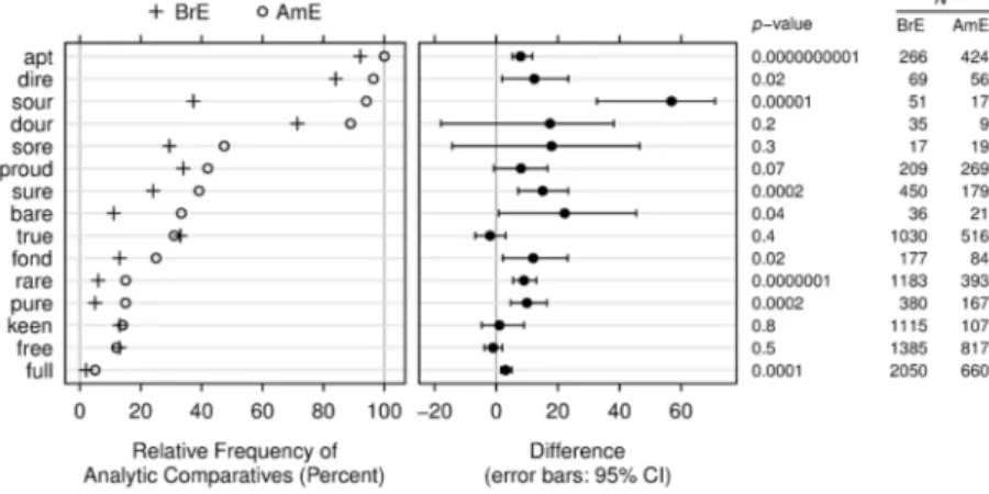
The dot plot: A graphical tool for data analysis and presentation
29
0
0
Volltext
(2)
(3)
(4)
(5)
(6)
(7)
(8)
(9)
(10)
(11)
(12)
(13)
(14)
(15)
(16)
(17)
(18)
(19)
(20)
(21)
(22)
(23)
(24)
(25)
(26)
(27)
(28)
(29)
Abbildung


+7


ÄHNLICHE DOKUMENTE
– The user defines the final number of control volumes (5 for example) – Grouping based on a connection ratio:. volume of
CentropeSTATISTICS joins data from the regions Vysocina, Jihomoravsky, Bratislavsky, Trnavsky, Györ-Moson-Sopron, Burgenland, Lower Austria, and Vienna and features
Die hier vorgestellten Arbeiten lassen sich unter drei breit gefasste Themenfelder subsumieren: Die ersten drei Beiträge thematisieren die Bedeutung des Kontextes für
Finally, in this section presenting exemplars of data re-use, Louise CORTI and Libby BISHOP reflect on the current published literature and existing training provision for
Mögen dies auch noch die letzten Ausläufer der 68-er-Jahre gewesen sein, so ist es doch beeindruckend, welche Vielfalt und Ebenbürtigkeit, wenn nicht gar Überlegenheit sich im
Der Beitrag beschäftigt sich im ersten Teil mit Chancen und Grenzen der Nutzung multicodaler Daten für die Analyse unter besonderer Berücksichtigung der Möglichkeiten, die sich
The initial aim of the documentation being a reproducible assessment of relevant parameters as complete as possible including the possibility of a concise illustration and storage
FAO-CIHEAM Mountain Pastures Network 16 th Meeting – Krakow - 2011.. Presentation of the Mountain Pastures
