Research Collection
Conference Paper
Imitation Learning from MPC for Quadrupedal Multi-Gait Control
Author(s):
Reske, Alexander; Carius, Jan; Ma, Yuntao; Farshidian, Farbod; Hutter, Marco Publication Date:
2021
Permanent Link:
https://doi.org/10.3929/ethz-b-000476607
Originally published in:
http://doi.org/10.1109/ICRA48506.2021.9561444
Rights / License:
In Copyright - Non-Commercial Use Permitted
This page was generated automatically upon download from the ETH Zurich Research Collection. For more information please consult the Terms of use.
ETH Library
Imitation Learning from MPC for Quadrupedal Multi-Gait Control
Alexander Reske, Jan Carius, Yuntao Ma, Farbod Farshidian, Marco Hutter
Abstract— We present a learning algorithm for training a single policy that imitates multiple gaits of a walking robot. To achieve this, we use and extend MPC-Net, which is an Imitation Learning approach guided by Model Predictive Control (MPC).
The strategy of MPC-Net differs from many other approaches since its objective is to minimize the control Hamiltonian, which derives from the principle of optimality. To represent the policies, we employ a mixture-of-experts network (MEN) and observe that the performance of a policy improves if each expert of a MEN specializes in controlling exactly one mode of a hybrid system, such as a walking robot. We introduce new loss functions for single- and multi-gait policies to achieve this kind of expert selection behavior. Moreover, we benchmark our algorithm against Behavioral Cloning and the original MPC implementation on various rough terrain scenarios. We validate our approach on hardware and show that a single learned policy can replace its teacher to control multiple gaits.
I. INTRODUCTION
The control of hybrid, underactuated walking robots is a challenging task, which becomes especially difficult in missions that require onboard real-time control. In this sce- nario, training a feedback policy offline with demonstrations from Optimal Control (OC) or Model Predictive Control (MPC) [1]–[3] is a promising option, as it combines the advantages of both data-driven and model-based approaches:
a learned policy computes control inputs quickly online, while OC provides a framework to find control inputs that respect constraints and optimize a performance criterion.
When a quadrupedal robot is deployed in different en- vironments, it can be advantageous to adapt the gait. For example, one might prefer a statically stable over a dynam- ically stable gait on uneven or slippery ground. However, in Reinforcement Learning (RL), policies often converge to a single gait [4], [5] with a few exceptions [6], [7]. Further, works on Imitation Learning (IL) usually try to imitate one behavior per policy [8], [9], making transitioning between policies difficult, as for a walking robot, switching between policies for different behaviors can cause jerky and unstable locomotion [7] unless one undesirably uses the stance mode for transitioning. One solution is to use policy distillation to merge multiple task-specific policies into a single pol- icy [10]. An alternative is to add task-specific signals to the observation space of a generic policy [7]. Motivated by this alternative, our approach can train a single feedback policy
This work was supported by the Swiss National Science Foundation (SNSF) through project 166232, 188596, the National Centre of Competence in Research Robotics (NCCR Robotics), and the European Union’s Horizon 2020 (grant agreement No.852044). Moreover, this work has been conducted as part of ANYmal Research, a community to advance legged robotics.
All authors are with the Robotic Systems Lab, ETH Z¨urich, Switzerland.
Email:areske@ethz.ch
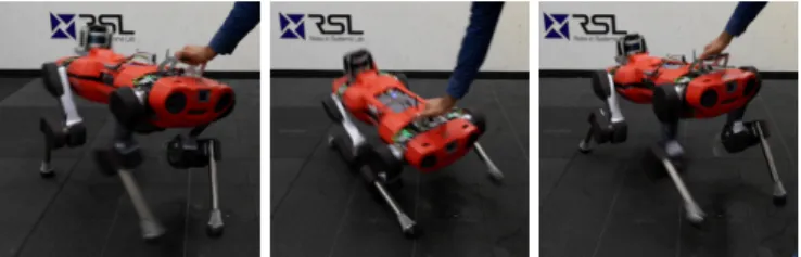
Fig. 1. ANYmal being pushed around while running a learned policy.
that imitates multiple gaits from MPC demonstrations and can switch between different gaits during execution.
Typically, IL approaches can be categorized into two groups [11]: Behavioral Cloning (BC) [12] replicates the demonstrator’s policy from state-input pairs without inter- acting with the environment, while Inverse Reinforcement Learning (IRL) [13] seeks to learn the demonstrator’s cost or reward function, which is subsequently used to train a policy with a standard RL procedure. In contrast, our work is based on MPC-Net [3], which is an IL approach that uses solutions from MPC to guide the policy search and attempts to minimize the control Hamiltonian, which also encodes the constraints of the underlying OC problem. MPC-Net differs from BC, as our learner is never presented with the optimal control input, and from IRL, as our cost function is obtained from a model-based controller instead of learning it.
The multi-modal nature of hybrid systems, such as walk- ing robots, motivates the use of a mixture-of-experts net- work (MEN) architecture [14] for representing the control policy [3], [15]. In this work, we provide further evidence that the performance of a policy improves if each expert of a MEN specializes in controlling exactly one mode of a hybrid system. This poses the challenge to reliably achieve such a single responsibility expert selection behavior, i.e., the MEN has to partition the problem space such that a single expert is responsible for a distinct mode. To this end, we introduce a new Hamiltonian loss function, which, compared to our previous work, leads to a better localization of the experts and, in turn, better performance on the robot. Moreover, in more complex multi-gait settings, we show how a guided loss function provides a framework for directing the learner with domain knowledge towards advantageous expert selections.
While our previous work [3] has established the underly- ing theoretical principle of a Hamiltonian loss function for policy search, this work contributes the following advances:
• Introduction of a new Hamiltonian loss function leading to a better localization of the MEN’s experts (III-A).
• Proposal of a guided loss function that allows the incorporation of domain knowledge for an improved expert selection strategy (III-B).
• Demonstration of the new Hamiltonian loss function resulting in improved performance (V-A).
• Benchmarking experiments confirming that MPC-Net leads to more robust policies compared to BC (V-B).
• Results showing that a single policy can learn multiple gaits and execute them with high performance (V-C).
II. BACKGROUND
This section covers the underlying control problem and recaps the main methodological aspects of the MPC-Net approach.
A. Model Predictive Control
MPC provides solutions to the following OC problem minimize
u(·) φ(x(tf)) + Z tf
ts
l(x(t),u(t), t) dt, (1)
subject to x(ts) =xs, (2a)
˙
x=f(x,u, t), (2b) g(x,u, t) =0, (2c) h(x,u, t)≥0, (2d) where x(t) and u(t) are the state and input at time t.
The objective is to minimize the final cost φ and the time integral of the intermediate cost l over the receding time horizonth=tf−ts, wheretsis the start time andtf is the final time. The initial statexs is given, and the system dy- namics are determined by the system flow mapf. Moreover, the minimization is subject to the equality constraintsg and the inequality constraintsh.
For the optimization, we use a Sequential Linear-Quadratic (SLQ) algorithm [16], which is a variant of the Differential Dynamic Programming (DDP) algorithm [17, p. 570]. The equality constraints g are handled using Lagrange multipli- ers ν [16], and the inequality constraints h are considered through a barrier functionb[18]. Therefore, the correspond- ing Lagrangian is given by
L(x,u, t) =l(x,u, t) +ν(x, t)>g(x,u, t)
+X
i
b(hi(x,u, t)). (3) The solution to the OC problem (1, 2) can be represented by a linear control policy based on the nominal state trajec- tory xnom(·), the nominal input trajectory unom(·), and the time-varying linear feedback gainsK(·)as
πmpc(x, t) =unom(t) +K(t)(x−xnom(t)). (4) Moreover, the optimal cost-to-go functionV and the control HamiltonianHcan be written respectively as
V(x, t) = min
u(·) s.t. (2)
φ(x(tf)) + Z tf
t
l(x(τ),u(τ), τ) dτ
, (5) H(x,u, t) =L(x,u, t) +∂xV(x, t)f(x,u, t), (6) where the Hamiltonian satisfies the well-known Hamilton- Jacobi-Bellman (HJB) equation for allt andx
0 = min
u {H(x,u, t) +∂tV(x, t)}. (7)
B. MPC-Net
The main idea of MPC-Net [3] is to imitate MPC by mini- mizing the Hamiltonian while representing the corresponding control inputs by a parametrized policyπ(x, t;θ). From the SLQ solver we have a local solutionV(x, t)for (7) as well as access to its state derivative ∂xV(x, t) and the optimal Lagrange multipliers ν(x, t). Therefore, finding a locally optimal control policy simplifies to minimizing the right- hand-side of (7) [19, p. 430]. This motivates the strategy for finding the optimal parametersθ∗, which is given by
θ∗= arg min
θ E{t,x}∼P[H(x,π(x, t;θ), t)], (8)
where the distributionP encodes which areas of the time- state space are visited by an optimal controller. The key training steps of this IL approach are schematically shown in Fig. 3 and are discussed in more detail in Sec. IV-E.
As the SLQ solver provides a local approximation of the optimal cost-to-go function and of the optimal Lagrange multipliers, MPC-Net takes samples around the nominal state to augment the data set. This reduces the number of MPC calls needed to successfully train a control policy and makes the learned policy more robust.
To address the mismatch between the distributions of states visited by the optimal and learned policy [20], MPC-Net forward-simulates the system with the behavioral policy
πb(x, t;θ) =απmpc(x, t) + (1−α)π(x, t;θ), (9) where the mixing parameterα linearly decreases from one to zero in the course of the training.
As mentioned in Sec. I, for hybrid systems, it is beneficial to represent the policy by a MEN architecture. Therefore, the output of the network is the policy
π(x, t;θ) =
E
X
i=1
pi(x, t;θ)πi(x, t;θ), (10) where the expert weightsp= (p1, . . . , pE)are calculated by a gating network and each expert policyπi is computed by one of theE experts.
Inserting (10) into (8) leads to the loss function L1=H x,
E
X
i=1
pi(x, t;θ)πi(x, t;θ), t
!
. (11) However, this loss results in cooperation rather than competi- tion between the experts. To encourage expert specialization, it is better to force each expert to individually minimize the objective [14]. For MPC-Net, this leads to the loss function
L2=
E
X
i=1
pi(x, t;θ)H(x,πi(x, t;θ), t). (12) Training the policy requires the gradient of the loss func- tion w.r.t. the parameters. For better readability, we define
pi=pi(x, t;θ), (13) Hi=H(x,πi(x, t;θ), t). (14)
Then, the gradient of (12) is
∂L2
∂θ =
E
X
i=1
pi
∂Hi
∂u
∂πi
∂θ +Hi
∂pi
∂θ, (15)
where the input derivative of the Hamiltonian ∂uHi can be queried from the SLQ solver, and the gradients ∂θπi and∂θpi are computed by backpropagation.
III. METHOD
In this section, we first introduce the new Hamiltonian loss function and then the guided loss function.
A. Log-Partitioned Loss Function
In a least-squares setting, Jacobs et al. [14] discuss a third MEN loss function, which is the negative log probability of a Gaussian mixture model and reportedly results in a better performance. Inspired by that, we introduce the loss function
L3=−1 β log
E
X
i=1
piexp (−β(Hi+∂tV))
!
, (16) where∂tV =∂tV(x, t)is a bias term motivated by (7) and computed by numerical differentiation, and β is an inverse temperature parameter. Note that the sum in the argument of the logarithm has some similarity to a partition function.
The expert weight pi can be seen as the prior probability that expert i can minimize the Hamiltonian at the current observation. In that light, we define the posterior probability
qi=qi(x, t;θ) := piexp (−β(Hi+∂tV))
E
P
j=1
pjexp (−β(Hj+∂tV))
, (17)
which is a better estimation of the probability that expert i can minimize the Hamiltonian. Then, the gradient of (16) can be written as
∂L3
∂θ =
E
X
i=1
qi
∂Hi
∂u
∂πi
∂θ − 1 β
qi
pi
∂pi
∂θ. (18)
Compared to (15), the expert updates are weighted by the posterior instead of the prior. Moreover, notice the difference in the sign of the gating updates. In (15) the expert weightpi receives a penalty given by the size of the corresponding Hamiltonian, whereas in (18) the expert weight pi receives a reward according to the ratio of the posterior and prior probabilities. In Sec. V-A we show that these properties indeed lead to improved performance.
To better understand the new loss function, note that we can also get (18) from the gradient of
E
X
i=1
¯ qiHi+1
β −
E
X
i=1
¯ qilog(pi)
!
, (19)
whereq¯i is equal toqi but detached from the computational graph, and thus no gradient will be backpropagated along this variable. The first term is similar to L2 but the expert weightpi is replaced by q¯i. The second term in parentheses is the cross-entropyCE(¯q, p)and pulls the prior towards the current posterior, which is fixed for the moment.
B. Guided Loss Function
To direct the learner with domain knowledge towards advantageous expert selections and influenced by the learning by cheating idea [21], we propose the guided loss
LG=LE+λLD, (20)
where LE ∈ {L1, L2, L3} is the expert loss, LD is a loss that incorporates the domain knowledge, and the parameterλ controls the relative importance of both loss types.
In the context of hybrid systems, the expert selection should be related to the mode selection in OC. The gait or mode selection either takes place based on optimization [22]
or based on other domain knowledge, such as qualification of the terrain [23] or commanded speeds [24]. In the simplest case, this leads to a mode schedule m(t) that returns the active modei at any timet. In general, however, the mode selection m(x, t) can also depend on the current observed state x. In that case, we define the empirical probability to observe modeias
˜
pi= ˜pi(x, t). (21) To incorporate our domain knowledge that the experts and modes should match, we maximize the log-likelihood, which is equivalent to minimizing the cross-entropy [25, p. 129].
Thus, forL1 andL2,LD is given by the cross-entropy CE(˜p, p) =−
E
X
i=1
˜
pilog(pi). (22) ForL3, eq. (22) and the cross-entropy term in (19) can be in conflict if the posterior does not agree with the observed modes. To avoid this scenario, it is better to guideL3 with
CE(˜p, q) =−
E
X
i=1
˜
pilog(qi), (23) which, with the interpretation in (19), encourages the pre- dicted expert selection to match the observed mode selection.
In the MEN literature, one can distinguish between a mixture of implicitly localized experts (MILE) and a mixture of explicitly localized experts (MELE) [26]. MILE uses a competitive process to localize the experts. For example,L2
and L3 belong to this group. In contrast, MELE assigns the experts to pre-specified clusters. In a broader sense, the guided loss LG can be seen as part of the MELE group. However, note that our method is different from hardcoding the assignment of the experts according to some heuristic and training separate networks for each case, as we allow the modes and their probabilities to be a function of the observations. Therefore, in this framework, the gating network can learn to deviate from a heuristic, such as a mode schedule for a hybrid system, and adapt the expert selection to the current observations. The benefits of the guided loss idea become evident in Sec. V-C.
Finally, it should be noted that a limitation of the presented methodology is that it requires a mode schedule. To address this limitation, one could try to learn a state-based mode selectionm(x), similar to works that predict mode schedules from states to facilitate solving the OC problem [27].
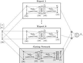
Fig. 2. MEN architecture instantiated for the ANYmal robot.
IV. IMPLEMENTATION
This section presents how the method is applied to a quadrupedal robot. Moreover, we explain our policy archi- tecture, the training procedure, and the deployment pipeline.
A. ANYmal Control
In this work, we use the quadrupedal robot ANYmal (Fig. 1), which is a hybrid system due to discrete switches in the contact configuration. The feet are constrained to have zero contact forces in the swing phase and zero velocity in the contact phase. For MPC, the robot is represented by a kinodynamic model, which has 24states (base pose, base twist, joint positions) and24inputs (foot contact forces, joint velocities) [16]. The OC cost function (1) is determined by φ(x) = (x−xd(tf))>Qf(x−xd(tf)), (24) l(x,u, t) = (x−xd(t))>Q(x−xd(t)) +u>R u, (25) where xd(·) is a desired state trajectory that should be tracked. We consider two gaits: trot, moving the diagonal legs together, and static walk, moving one leg at a time. So, including the stance mode, we have to controlM = 7modes.
B. Gait Parametrization
Based on the absolute time and the current state, it is difficult for the learned policy to infer which legs should be moved. Therefore, it is more direct to provide a parametriza- tion of the gait. From the mode schedule we extract the leg phasesϕ= (ϕLF, ϕRF, ϕLH, ϕRH)according to
ϕi=
t−tlo
ttd−tlo
, if leg iin swing, 0, if leg iin contact,
(26) wheretlois the liftoff andttdthe touchdown time. By abuse of notation, we replace the absolute timetin the policy (10) with the so-called generalized time
t=
ϕ ϕ˙ sin(πϕ)>
. (27)
The sinusoidal bumpssin(πϕ)[3] provide a reference for the swing motion. We add the leg phasesϕto learn asymmetries between the liftoff and touchdown phase and their time derivativesϕ˙ to capture different swing speeds. We address the benefits of this parametrization in Sec. V-A.
Fig. 3. Schematic of the MPC-Net training procedure.
C. Relative State
For reference tracking, we replace the state x in the policy (10) with a tracking error called the relative state
xr(t) =T(θB) (x−xd(t)), (28) whereθB is the current orientation of the base in the world frame and the matrixT(θB)transform the pose error from the world into the base frame to make the policy training and deployment invariant w.r.t. the absolute orientation.
D. Policy Architecture
The MEN architecture for the policies is shown in Fig. 2.
We use E = 8 Multilayer Perceptron (MLP) experts and a MLP gating network with a softmax output activation, which ensures that the expert weights p are positive and sum to one. Note that as long as E ≥ M, training and deployment are not sensitive w.r.t. the parameter E, and the gating network is able to learn to select an appropriate expert for the mode [3]. For example, we also trained policies withE= 12experts but could not observe an advantage in terms of expert selection or policy performance.
Carius et al. [3] use an architecture with a common hidden layer for linear experts and a linear gating network, which has a sigmoid output activation with a subsequent normal- ization. While we postulate that the common hidden layer is beneficial for training from little demonstration data, we use several MLP experts since this allows the expert networks to extract distinct features for the individual modes that they are responsible for. In combination with the loss functionL2, the normalized sigmoids help to select a consistent number of experts [3]. However, the more common softmax better corresponds to the concept of single responsibility, and we handle the issue of expert selection with the newly introduced loss functionsL3 andLG.
E. Training
The training procedure is schematically shown in Fig. 3.
First, note that the multi-threaded data generation and the policy search run asynchronously. While MPC-Net can sta- bilize different gaits from less than 10 min of demonstration data [3], the multi-threaded data generation ensures that the amount of data is not a bottleneck in this work.
Data are generated byntthreads that work onnj jobs per data generation run. For each job, we start from a random initial statex0with the task to reach a desired statexdwithin the rollout lengthT. In a loop, we run MPC, save the data,
TABLE I
HYPERPARAMETERS OFMPC-NET.
time step∆t 0.0025 s inverse temperatureβ 1.0 rollout lengthT 4 s guided loss weightλ 1.0 number of threadsnt 5 number of expertsE 8
number of jobsnj 10 batch sizeB 32
number of samplesns 1 learning rateη 1e-3 data decimationdd 4 iterations single-gaitis 100k metrics decimationdm 200 iterations multi-gaitim 200k
and forward simulate the system by the time step ∆t. To avoid storing data that have similar informational content, we downsample the data and thus only save the nominal data and the data fromnssamples around the nominal state in everydd-th step. A rollout is considered as failed, and its data are discarded if the pitch or roll angle exceeds 30◦or if the height deviates more than 20 cm from the default value.
If a data generation run has completed, the data are pushed into the learner’s replay buffer of size N. In every learning iteration, we draw a batch of B tuples {t,xr, ∂tV, ∂xV,ν}
from the replay buffer, compute the empirical cost J(θ) = 1
B
B
X
j=1
L(tj,xr,j, ∂tVj, ∂xVj,νj,θ), (29) whereL∈ {L1, L2, L3, LG}, and perform a gradient descent step in the parameter space using the Adam optimizer [28].
To monitor the training progress and as a substitute for a validation set, we perform a rollout with the learned policy at everydm-th iteration and compute the following metrics:
the average constraint violation, the incurred cost (1), and the survival time until our definition of failure applies.
When using the system dynamicsf for the rollouts [3], it is possible that the learned policy cheats, e.g., by applying forces in mid-air. In this work, we use the physics engine RaiSim [29] for the data generation and metrics rollouts. The availability of more realistic training data improves the sim- to-real transfer, and using a physics engine for validation leads to more accurate metrics of true performance. The mentioned hyperparameters are summarized in Table I.
F. Deployment
Simply put, the learned policy replaces MPC in our control architecture. More specifically, our controller is given a mode schedule, the current state x, and a desired state xd, which is generated from the user’s commands (Fig. 4). From these quantities, the relative state xr and the generalized time t can be assembled and passed into the policy network. The kinodynamic control inputs u, which are inferred from the learned policyπusing ONNX Runtime [30], are tracked by a whole-body controller (WBC) that computes the actuator torque commandsτ [31].
Fig. 4. Deployment pipeline with the policy module replacing MPC.
TABLE II
ABILITY OF THE LOSSL2ANDL3TO ACHIEVE SINGLE RESPONSIBILITY OF THE EXPERTS FOR THE MODES OF TROT AND STATIC WALK. THE
SHOWN PERCENTAGES ARE BASED ON TEN TRAINING RUNS EACH.
L2 L3
β= 0.5 β= 1.0 β= 2.0
trot 40% 100% 100% 50%
static walk 0% 40% 90% 70%
V. RESULTS
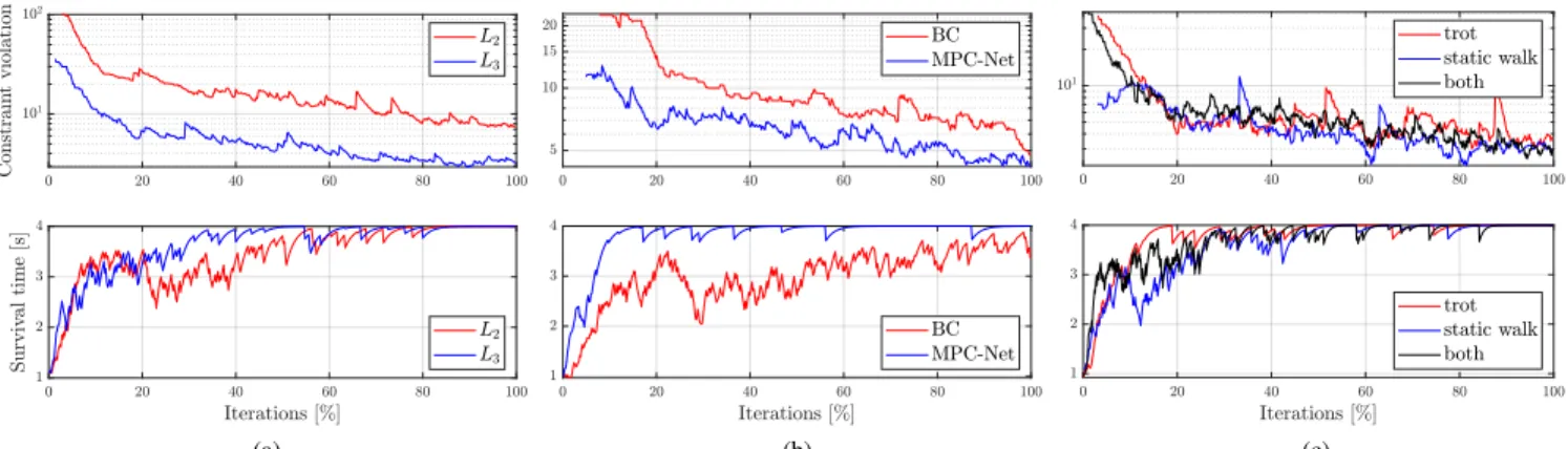
In this section, we show how our methodological contri- butions and implementation details lead to improved results compared to prior work. To assess the performance of a learned policy, we found that the survival time and the constraint violation computed from the metrics rollouts are good indicators. For the actual performance on hardware, we refer to the supplementary video1. In the presented plots, noisy data, e.g., from the metrics rollouts, are filtered by an exponential moving average filter with smoothing factor0.9.
A. Ablation Study
We begin by providing evidence that the generalized timet and the new loss L3 help the MPC-Net algorithm to find better policies compared to our previous work [3].
Extending the gait parameterizationsin(πϕ)withϕandϕ˙ reduces the constraint violation by a factor of four. As theϕ˙ are rectangular functions, we conjecture that they facilitate changing experts at mode switches and, ergo, learning to respect the constraints of the swing and contact phases.
In Fig. 5a we compare the lossL2 with the new lossL3, which achieves a lower constraint violation as well as a faster increase in the survival time. Note that in Fig. 5a the policy trained with the lossL2 only employs three experts, where one expert is responsible for the stance and two static walk modes. Based on many experiments and as indicated by Fig. 5a, we conclude that the performance of a policy improves if each expert of a MEN specializes in controlling exactly one mode of a hybrid system. Table II shows that the new loss L3 is better at achieving this single responsibility expert selection in general and especially for our choice of the inverse temperatureβ= 1.0. We observe that the gating network commits to a certain expert selection early in the training process, which highlights the importance of efficient gradient updates as given by (18).
B. Benchmarking
We benchmark our algorithm against the original MPC and BC. For the latter, we replace the Hamiltonian and the bias term inL3with the normalized mean-squared error from the model predictive controller’s control commands.
In Fig. 5b we compare the MPC-Net algorithm with BC, whose policies do not persistently reach the desired survival time of 4 s. Note that only completed metrics rollouts are considered in the constraint violation plots. In this respect, policies trained with BC attain a slightly larger constraint violation for the rollouts that they survive but fail for rollouts
1Link:https://youtu.be/AUNIhr5I6Dg
(a) (b) (c)
Fig. 5. The top graphs show a comparison of the constraint violation and the bottom graphs a comparison of the survival time. In this figure, all policies trained with lossL3achieve single responsibility of the experts for the modes. (a) Performance of static walk when training with lossL2orL3. (b) Performance of trot when using the BC or MPC-Net training approach. (c) Performance of a multi-gait policy consisting of trot and static walk compared to the corresponding single-gait policies. Note that the multi-gait training goes through twice as many iterations, and the policies can also control the pose.
TABLE III
SURVIVAL TIME(MEAN AND STANDARD DEVIATION)WHEN DEPLOYING MPC, MPC-NET,ANDBCPOLICIES ON TERRAIN WITH DIFFERENT
SCALES OF ROUGHNESS BASED ON FIFTY TEST RUNS EACH.
z-scale [29] MPC MPC-Net BC
0.0 20.0±0.0 20.0±0.0 20.0±0.0 4.0 19.2±2.6 18.9±2.9 6.8±4.5 8.0 12.2±5.6 10.6±6.3 2.6±1.6
with apparently more difficult tasks {x0,xd} that only policies trained with MPC-Net complete successfully.
To quantify the robustness of the approaches, we deploy MPC as well as policies trained with MPC-Net and BC on rough terrain in RaiSim, command them to walk forward for at most 20 s, and measure the survival time. Table III shows that policies trained with MPC-Net outperform those trained with BC in surviving rough terrain, which was not part of the training data. While the effects are difficult to isolate, we imagine MPC-Net shows comparatively greater robustness by learning from the Hamiltonian, which also encodes the constraints that ensure physical feasibility. Compared to MPC, MPC-Net achieves similar survival times. We think that learning from MPC simulated at 400 Hz enables the policy to compete with MPC running at 40 Hz, which is an achievable onboard update frequency for MPC on ANYmal.
C. Multi-Gait Policy
With our approach, a single policy can learn multiple gaits and execute them with high performance. Fig. 5c shows that a multi-gait policy achieves a constraint violation and a survival time that are similar to the corresponding single-gait policies. Also, on hardware, we observe similar performance.
Unfortunately, in multi-gait scenarios,L3does not reliably achieve single responsibility. We observe that the network tends to commit too early to too few experts and conjecture that the Hamiltonian does not provide enough discrimination to reliably identify all modes. Therefore, we propose to encode the single responsibility with the guided lossLG. In that case, the guided versions ofL1,L2, andL3all achieve single responsibility and thus similar performance to the multi-gait policy shown in Fig. 5c. Fig. 6 shows the expert selection for a policy trained with the guided loss LG. In
Fig. 6. Expert selection in simulation (left) and on hardware (right) for a multi-gait policy trained with the guided lossLG. The robot starts in stance (blue) and then alternates between trot (orange, yellow) and static walk (purple, red, green, light blue). One expert (black) is not used.
simulation, one can see that the expert selection corresponds to the mode schedule due to the single responsibility. On hardware, the expert selection slightly deviates from the plan.
For example, at the end of the second trot mode (yellow), one leg is in early contact, which activates one of the static walk experts (light blue) for a short moment.
While we deem trot and static walk to be the practically most relevant gaits, we tested in simulation how our method scales to more than two gaits. As shown in the video, we added a more exotic gait, namely dynamic diagonal walk, i.e., a hybrid of static walk and trot, to the multi-gait training.
In general, it can be noted that if the deployment deviates too much from the training data and especially if the execution requires new modes, such as for pace or bounding, then one has to explicitly train it and ensure that there are enough experts to cover all the modes of the gaits.
VI. CONCLUSION
In this work, we observed that the performance of a policy improves if each expert of a MEN specializes in controlling exactly one mode of a hybrid system. Motivated by this, we introduced a new loss function, which leads to better expert localization and thus almost always achieves single responsibility for single-gait policies. We showed that MPC- Net policies are comparatively robust. Moreover, our method and implementation enable a single policy to learn multiple gaits by the incorporation of domain knowledge through a guided loss function. Finally, we validated our approach on hardware and showed that the learned policies can replace MPC during deployment. This opens the door for more complicated scenarios that do not run in real time with MPC.
REFERENCES
[1] I. Mordatch and E. Todorov, “Combining the benefits of function ap- proximation and trajectory optimization,” inProceedings of Robotics:
Science and Systems (RSS) X. Robotics: Science and Systems, 2014.
[2] G. Kahn, T. Zhang, S. Levine, and P. Abbeel, “PLATO: Policy Learning using Adaptive Trajectory Optimization,” inProceedings of the 2017 IEEE International Conference on Robotics and Automation (ICRA). IEEE, 2017, pp. 3342–3349.
[3] J. Carius, F. Farshidian, and M. Hutter, “MPC-Net: A First Principles Guided Policy Search,”IEEE Robotics and Automation Letters, vol. 5, no. 2, pp. 2897–2904, 2020.
[4] T. Haarnoja, S. Ha, A. Zhou, J. Tan, G. Tucker, and S. Levine,
“Learning to Walk via Deep Reinforcement Learning,” inProceedings of Robotics: Science and Systems (RSS) XV. Robotics: Science and Systems, 2019.
[5] J. Hwangbo, J. Lee, A. Dosovitskiy, D. Bellicoso, V. Tsounis, V. Koltun, and M. Hutter, “Learning agile and dynamic motor skills for legged robots,”Science Robotics, vol. 4, no. 26, 2019.
[6] J. Tan, T. Zhang, E. Coumans, A. Iscen, Y. Bai, D. Hafner, S. Bohez, and V. Vanhoucke, “Sim-to-Real: Learning Agile Locomotion For Quadruped Robots,” inProceedings of Robotics: Science and Systems (RSS) XIV. Robotics: Science and Systems, 2018.
[7] A. Iscen, K. Caluwaerts, J. Tan, T. Zhang, E. Coumans, V. Sindhwani, and V. Vanhoucke, “Policies Modulating Trajectory Generators,” in Proceedings of the 2nd Conference on Robot Learning (CoRL).
PMLR, 2018, pp. 916–926.
[8] P. Abbeel, A. Coates, and A. Y. Ng, “Autonomous Helicopter Aero- batics through Apprenticeship Learning,”The International Journal of Robotics Research, vol. 29, no. 13, pp. 1608–1639, 2010.
[9] X. B. Peng, E. Coumans, T. Zhang, T.-W. Lee, J. Tan, and S. Levine,
“Learning Agile Robotic Locomotion Skills by Imitating Animals,” in Proceedings of Robotics: Science and Systems (RSS) XVI. Robotics:
Science and Systems, 2020.
[10] Z. Xie, P. Clary, J. Dao, P. Morais, J. Hurst, and M. Van De Panne,
“Learning Locomotion Skills for Cassie: Iterative Design and Sim- to-Real,” in Proceedings of the 3rd Conference on Robot Learning (CoRL). PMLR, 2019, pp. 317–329.
[11] T. Osa, J. Pajarinen, G. Neumann, J. A. Bagnell, P. Abbeel, and J. Pe- ters, “An Algorithmic Perspective on Imitation Learning,”Foundations and Trends in Robotics, vol. 7, no. 1-2, pp. 1–179, 2018.
[12] M. Bain and C. Sammut, “A Framework for Behavioural Cloning,” in Machine Intelligence 15: Intelligent Agents. Oxford University Press, 1999, pp. 103–129.
[13] P. Abbeel and A. Y. Ng, “Apprenticeship learning via inverse reinforce- ment learning,” inProceedings of the 21st International Conference on Machine Learning (ICML). ACM, 2004, pp. 1–8.
[14] R. A. Jacobs, M. I. Jordan, S. J. Nowlan, and G. E. Hinton, “Adaptive Mixtures of Local Experts,”Neural Computation, vol. 3, no. 1, pp.
79–87, 1991.
[15] H. Zhang, S. Starke, T. Komura, and J. Saito, “Mode-Adaptive Neural Networks for Quadruped Motion Control,” ACM Transactions on Graphics (TOG), vol. 37, no. 4, pp. 1–11, 2018.
[16] F. Farshidian, M. Neunert, A. W. Winkler, G. Rey, and J. Buchli, “An Efficient Optimal Planning and Control Framework For Quadrupedal Locomotion,” inProceedings of the 2017 IEEE International Confer- ence on Robotics and Automation (ICRA). IEEE, 2017, pp. 93–100.
[17] J. B. Rawlings, D. Q. Mayne, and M. M. Diehl,Model Predictive Control: Theory, Computation, and Design, 2nd ed. Nob Hill Publishing, 2017.
[18] R. Grandia, F. Farshidian, R. Ranftl, and M. Hutter, “Feedback MPC for Torque-Controlled Legged Robots,” in Proceedings of the 2019 IEEE/RSJ International Conference on Intelligent Robots and Systems (IROS). IEEE, 2019, pp. 4730–4737.
[19] D. P. Bertsekas,Dynamic Programming and Optimal Control, 4th ed.
Athena Scientific, 2017.
[20] S. Ross, G. J. Gordon, J. A. Bagnell, and M. Learning, “A Reduction of Imitation Learning and Structured Prediction to No-Regret Online Learning,” in Proceedings of the 14th International Conference on Artificial Intelligence and Statistics (AISTATS). JMLR W&CP, 2011, pp. 627–635.
[21] D. Chen, B. Zhou, V. Koltun, and P. Kr¨ahenb¨uhl, “Learning by Cheating,” inProceedings of the 3rd Conference on Robot Learning (CoRL). PMLR, 2019, pp. 66–75.
[22] A. W. Winkler, C. D. Bellicoso, M. Hutter, and J. Buchli, “Gait and Trajectory Optimization for Legged Systems Through Phase- Based End-Effector Parameterization,”IEEE Robotics and Automation Letters, vol. 3, no. 3, pp. 1560–1567, 2018.
[23] M. Brandao, O. B. Aladag, and I. Havoutis, “GaitMesh: Controller- Aware Navigation Meshes for Long-Range Legged Locomotion Plan- ning in Multi-Layered Environments,”IEEE Robotics and Automation Letters, vol. 5, no. 2, pp. 3596–3603, 2020.
[24] W. Xi, Y. Yesilevskiy, and C. D. Remy, “Selecting gaits for economical locomotion of legged robots,”The International Journal of Robotics Research, vol. 35, no. 9, pp. 1140–1154, 2016.
[25] I. Goodfellow, Y. Bengio, and A. Courville,Deep Learning. MIT Press, 2016.
[26] S. Masoudnia and R. Ebrahimpour, “Mixture of experts: A literature survey,” Artificial Intelligence Review, vol. 42, no. 2, pp. 275–293, 2014.
[27] F. R. Hogan and A. Rodriguez, “Reactive planar non-prehensile manipulation with hybrid model predictive control,”The International Journal of Robotics Research, vol. 39, no. 7, pp. 755–773, 2020.
[28] D. P. Kingma and J. L. Ba, “Adam: A Method for Stochastic Optimization,” inProceedings of the 3rd International Conference on Learning Representations (ICLR), 2015.
[29] J. Hwangbo, J. Lee, and M. Hutter, “Per-Contact Iteration Method for Solving Contact Dynamics,” IEEE Robotics and Automation Letters, vol. 3, no. 2, pp. 895–902, 2018. [Online]. Available:
www.raisim.com
[30] “ONNX Runtime: cross-platform, high performance ML inferencing and training accelerator.” [Online]. Available:
https://github.com/microsoft/onnxruntime
[31] C. D. Bellicoso, C. Gehring, J. Hwangbo, P. Fankhauser, and M. Hut- ter, “Perception-less Terrain Adaptation through Whole Body Control and Hierarchical Optimization,” inProceedings of the 2016 IEEE-RAS 16th International Conference on Humanoid Robots (Humanoids).
IEEE, 2016, pp. 558–564.