Lecture 12
Pulse Synchronization
In this lecture, we finally address the task of self-stabilizing pulse synchroniza- tion. A trace is good from time t if starting from then (i.e., when starting to count pulses from time t), the requirements of pulse synchronization are met.
We will head for an algorithm with a very good trade-o↵ between stabiliza- tion time and communication complexity — here measured by the amount of bits a correct node broadcasts within
O(d) time — right away. This will be achieved by reducing the task to consensus, very similar to the previous lecture. How- ever, the fact that timing is now imprecise (due to uncertain message delays and drifting clocks), the details become rather complex. We will focus on the key ideas in this lecture, deliberately avoiding to give detailed proofs. Once we strip away these obfuscating issues, very little conceptual di↵erences remain between the solution from the previous lecture and the algorithm presented today.
12.1 Outline of the Construction
We will sketch the overall construction, relying on the high similarity to the recursive construction of synchronous counting algorithms from the previous lecture for intuition. This will lead to identifying the main challenge in the approach, which we will focus on afterwards. Let us first state the final result of the machinery.
Theorem 12.1.
For f
2N0, denote by C(f ) (synchronous deterministic) con- senus algorithms tolerating f faults on any number n 3f + 1 of nodes and by R(f ) and M (f ) their round complexities and message sizes, respectively. If 1 <
#1.004, there exists T
0 2⇥(R(f)) and
'21 +
O(# 1) such that for any T T
0there is a pulse synchronization algorithm P satisfying that
•
it stabilizes in S(P )
2O(d(1 +
Pdlogfek=0
R(2
k))) time,
•
correct nodes broadcast M (P )
2O(1 +
Pdlogfek=0
M (2
k)) bits per d time,
•
it has skew 2d,
•
it has minimum period P
minT , and
•
it has maximum period P
max'T.137
Corollary 12.2.
If 1 <
#1.004, there exists T
02⇥(f) and
'21 +
O(# 1) such that for any T T
0there is a pulse synchronization algorithm P satisfying that
•
it stabilizes in
O(df) time,
•
correct nodes broadcast
O(log f ) bits per d time,
•
it has skew 2d,
•
it has minimum period P
minT , and
•
it has maximum period P
max'T.
Proof. We plug the Phase King algorithm into Theorem 12.1.
To make the recursion underlying this theorem work, again we need two main steps: The first is to construct pulse synchronization algorithms from resynchro- nization algorithms, which are “weak” pulse synchronization algorithms that produce a “proper” pulse only once in a while; the second is to construct resyn- chronization algorithms from two pulse synchronization algorithms on disjoint subsets of the nodes.
Definition 12.3
(Resynchronization Algorithm). B is an f -resilient resynchro- nization algorithm with skew
⇢and separation window that stabilizes in time S(B), if the following holds: there exists a time t
S(B) such that every correct node v
2V
glocally generates a resynchronization pulse at time r(v)
2[t, t +
⇢)and no other resynchronization pulse before time t +
⇢+
. We call such aresynchronization pulse good.
Here is an example on how this might look like:
Node 1 Node 2 Node 3 Node 4
good resynchronisation pulse
faulty node, arbitrary behaviour spurious pulses
t t+⇢ t+⇢+
no pulses for time
Note that we do not impose any restrictions on what the nodes do outside the interval [t, t +
⇢+
). In particular, in constrast to the synchronous countingconstruction, we do not require that correct nodes agree on whether there are pulses or not outside this interval. Instead, this part of the construction will be subsumed by the first step, in which we construct pulse synchronization algorithms from resynchronization algorithms.
Using the same ideas as in the previous lecture, one can construct resynchro- nization algorithms from two smaller pulse synchronization instances as follows:
•
Both instances may trigger resynchronization pulses via generating pulses.
•
The instances (are supposed to) run at di↵erent frequencies. Hence, re-
gardless of their initial phase relation, after a few pulses a correct instance
(i.e., one with sufficiently many correct nodes) is guaranteed to produce a
good pulse, provided that the other one adheres to its frequency bound.
•
All correct nodes will “echo” seeing a pulse from either instance and only accept it if (i) n f nodes echoed the pulse, (ii) it adheres to the frequency bounds according to the node’s local clock, and (iii) the node didn’t re- cently observe fewer than n f and more than f nodes echo a pulse of the instance.
•
If (i), (ii), or (iii) are violated, a node will (locally) suppress any pulses by the respective instance for sufficiently long to guarantee that the other (correct) instance succeeds in generating a good pulse.
As in the previous lecture, this forces a faulty instance to stick to the required frequency bound or be ignored entirely. It does not guarantee that all pulses are produced consistently (as we don’t run consensus), but this is not required from a resynchronization algorithm.
Once we also have a way of constructing pulse synchronization algorithms from resynchronization algorithms, which we will discuss in more depth, the recursive construction is performed exactly as for synchronous counting, cf. Fig- ure 12.1. For f = 0, pulse synchronization is trivial; all nodes simply trigger pulses when a designated leader tells them to. To construct an algorithm for f
2[2
i, 2
i+11], i
2 N, faults, we select f
0, f
1< 2
iso that f
0+ f
1+ 1 = f and (the already inductively constructed) pulse synchronization algorithms with n
0= 3f
0+ 1 and n
1= 3f
1+ 1 nodes, implying that n
0+ n
1< 3f + 1
n. From these we derive a resynchronization algorithm on all n nodes tolerating f faults, which in turn we use to obtain the desired pulse synchronization algorithm.
Working out the details, one arrives at the result stated in Theorem 12.1.
Remarks:
•
In Theorem 12.1,
'is a bit larger than
#, as the construction is lossy withrespect to the quality of the hardware clocks. However, up to constant factors, the quality of the clocks is preserved:
'1
2O(# 1).
•
The described construction of resynchronization algorithms is fraught with a frustating amount of bookkeeping due to the slightly di↵erent perception of time of the correct nodes. While the approach works just as described if
# 1.004 — a somewhat arbitrary bound that could be improved to a certain extent — formalizing the construction and proving it correct is very laborious.
•
Accordingly, we will not do this in this lecture, but rather focus on the other main step of the recursive construction, in which we get to see some new algorithmic ideas.
12.2 Stabilization after Resynchronization Pulse
Before getting to business, let’s have a look at the general setting and a few no-
tational simplifications. First, assume that at time 0 each node locally triggers
a good resynchronization pulse, where “is large enough” for the stabiliza-
tion process to finish before any other resynchronization pulse, good or bad, is
triggered at a correct node (the minor time di↵erence of up to between the
resynchronization pulses can easily be accounted for, so we neglect it here). We
need to guarantee that within time the algorithm stabilizes and cannot be
P(7, 2): pulse synchronisation algorithm (Theorem 6) B(7, 2): resynchronisation algorithm (Theorem 7) P(4, 1): pulse synchronisation algorithm (T6) B(4, 1): resynchronisation algorithm (T7)
P(2, 0) P(2, 0)
P(3, 0): trivial pulse synchronisation algorithm
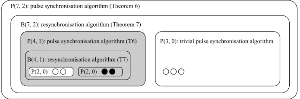
Figure 12.1: Recursively building a 2-resilient pulse synchronization algorithm P (7, 2) over 7 nodes. The construction utilises low resilience pulse synchro- nization algorithms to build high resilience resynchronization algorithms, which can then be used to obtain highly resilient pulse synchronization algorithms.
Here, the base case consists of trivial 0-resilient pulse synchronization algo-
rithms P(2, 0) and P (3, 0) over 2 and 3 nodes, respectively. Two copies of
P (2, 0) are used to build a 1-resilient resynchronization algorithm B(4, 1) over 4
nodes using. The resynchronization algorithm B(4, 1) is used to obtain a pulse
synchronization algorithm P (4, 1). Now, the 1-resilient pulse synchronization
algorithm P (4, 1) over 4 nodes is used together with the trivial 0-resilient algo-
rithm P(3, 0) to obtain a 2-resilient resynchronization algorithm B(7, 2) for 7
nodes and the resulting pulse synchronization algorithm P(7, 2). White nodes
represent correct nodes and black nodes represent faulty nodes. The gray blocks
contain too many faulty nodes for the respective algorithms to correctly operate,
and hence, they may have arbitrary output.
“confused” by any inconsistent resynchronization pulses. Accordingly, we will make sure that resynchronization pulses can a↵ect the behavior of nodes only when the algorithm has not already stabilized.
Our approach to generating pulses will be to execute consensus for each pulse. The challenge is to stabilize this procedure.
Simulating Consensus
We want to run synchronous consensus, but we’re not operating in the syn- chronous model. Hence, we need to simulate synchronous execution. To this end, we may use any (non-stabilizing) pulse synchronization algorithm, where we locally count the pulses to keep track of the round number. This works splen- didly, provided that each run is initialized correctly: using the Srikanth-Toueg algorithm (cf. Task 3 of exercise sheet 10), if all correct nodes start execution of the pulse synchronization algorithm within a time window of
O(Rd) time, simulation of an R-round consensus algorithm can be completed within
O(Rd) time; the outputs will even be generated within
O(d) time, as the skew of the algorithm is 2d. We will never need more than one instance to run, so this will be efficient in terms of communication.
However, as nodes may initially be in arbitrary states, the simulation may get “messed up,” at least until we can clear the associated variables and (re- )initialize them properly. This is the first challenge we need to overcome. In addition, we may also run into the familiar issue that not all correct nodes may know that they should simulate an instance. In this case, the pulse synchro- nization algorithm may not even function correctly. All of these problems will essentially be solved by employing silent consensus. Either all correct nodes participate, which causes them to reinitialize all state variables of the simu- lated consensus routine and ensures that the pulse synchronization algorithm works correctly, or no correct node will send messages for the consensus rou- tine — meaning that it will never output 1 (the only result that matters), even if the simulation is completely o↵ in terms of timing and attribution of mes- sages to rounds due to the Srikanth-Toueg algorithm breaking. Summarizing, the simulation has the following properties
•
Each node stores the state of at most one consensus instance. It aborts any local simulation if its local clock shows that it has been running for longer than the maximum possible time of T
max2O(Rd).
•
If all correct nodes initialize an instance within
⌧ 2 O(Rd) time (for a suitable relation between
⌧and T
max) and none of them re-initialize for another instance, all correct nodes will terminate within T
maxtime and produce an output satisfying validity and agreement.
•
If during (t d, t] no correct node is simulating an instance (i.e., by time
t there are also no more respective messages in transit), no correct node
will output a 1 as result of a simulation during (t d, t
1+ T
min], where
t
1is the infimal time larger than t d when a correct node initializes
an instance with input 1 and T
min 2 ⇥(Rd) is the minimum time tocomplete simulation of a consensus instance (note that we can enforce
such a minimum time even for “incorrect” execution, by having nodes
check the timing locally).
G1’
G2 G2 G1 G2’
������� �����
����
Guard Condition
G1 hT1iexpires and received n f �����messages within timeT1beforeT1expired
G1’ hT1iexpires and¬G1
G2 auxiliary machine signals������1 G2’ hTwaitiexpires or
auxiliary machine signals������0
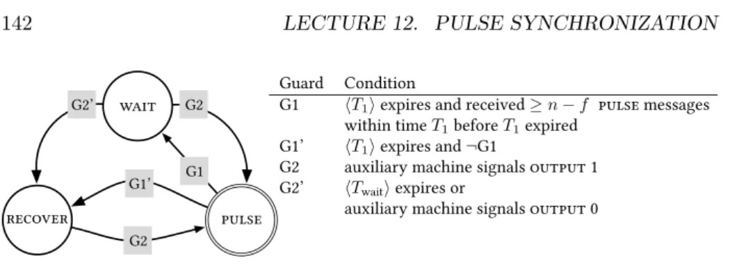
Figure 12.2: The main state machine. When a node transitions to state pulse (double circle) it will generate a local pulse event and send a pulse message to all nodes. When the node transitions to state wait it broadcasts a wait message to all nodes. Guard G1 employs a sliding window memory bu↵er, which stores any pulse messages that have arrived within time T
1(as measured by the local clock). When a correct node transitions to pulse it resets a local T
1timeout. Once this expires, either Guard G1 or Guard G1’ become satisfied.
Similarly, the timer T
waitis reset when node transitions to wait. Once it expires, Guard G2’ is satisfied and node transitions from wait to recover. The node can transition to the pulse state when Guard G2 is satisfied, which requires an output 1 signal from the auxiliary state machine given in Figure 12.3.
Remarks:
•
A formal proof would require to work out the constants and how they relate to each other. However, as we know that
#is “sufficiently close” to 1, tweaking the period of the Srikanth-Toueg algorithm the right way, we can assume that T
max⇡T
min+
⌧.State Machines
Our overall strategy is simple. Once stabilized, the algorithm generates pulses by repeatedly executing consensus instances, where each correct node will use input 1, and an output of 1 triggers a pulse. To this end, each node runs a copy of the main state machine shown in Figure 12.2. All correct nodes will see each other generating a pulse within T
1 2 ⇥(d) local time, transition towait, and this will ultimately result in the next consensus instance being initialized by the auxilliary state machine (shown in Figure 12.3).
To achieve stabilization, we seek to enforce one of two events: either (i) a
consensus instance is simulated correctly, outputs 1 (by agreement at all nodes),
and thus generates a synchronized pulse kicking the system back into the in-
tended mode of operation, or (ii) all nodes end up in state recover of the
state machine. A node being in state recover means that it has proof that the
algorithm has not stabilized (yet) and may thus take actions that are caused
by a resynchronization pulse, as this does not jeopardize stable operation in
case of spurious resynchronization pulses. Therefore, if we ensure that within
O(dR) time after a good resynchronization pulse either (i) occurs or (ii) hap-
pens and no consensus instance is running anymore (or about to be started), we
can “restart” the system by letting each correct node in state recover start
G4
G3
G6 G6’
G5 G5’
G7 G9
G9
G8 G8
G4 G4
������1
������0
Guard Condition
G3 hTactiveiexpires while in�������
G4 f+ 1����messages within timeTlisten
G5 n f����messages within timeTlisten
G5’ hTlisteniexpires
Guard Condition
G6 hT2iexpires while not in�������
G6’ hT2iexpires while in�������
G7 hT2iexpires G8 Aoutputs ‘1’
G9 Aoutputs ‘0’orhTconsensusiexpires or G4 is satis�ed
������ ����
�����0
�����1 ���1
���0
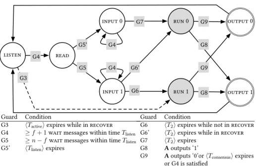
Figure 12.3: The auxiliary state machine. The auxiliary state machine is re-
sponsible for initializing and simulating the consensus routine. The gray boxes
denote states which represent the simulation of the consensus routine C. If the
node transitions to run 0, it uses input 0 for the consensus routine. If the node
transitions to run 1, it uses input 1. When the consensus simulation declares
an output, the node transitions to either output 0 or output 1 (sending the
respective output signal to the main state machine) and immediately to state
listen. The timeouts T
listen, T
2, and T
consensusare reset when a node transi-
tions to the respective states that use a guard referring to them. The timeout
T
activein Guard G3 (dashed line) is reset by the resynchronisation signal from
the underlying resynchronisation algorithm. Both input 0 and input 1 have a
self-loop that is activated if Guard G4 is satisfied. This means that if Guard G4
is satisfied while in these states, the timer T
2is reset.
a consensus instance with input 1, simply when a sufficiently large timeout of
⇥(dR) expires.
Either way, a pulse with small skew will be generated, from which on the system will run as intended.
Lemma 12.4.
Suppose that all correct nodes transition to pulse during [t, t + 2d] and timeouts are suitably chosen. Then the execution stabilized by time t, where a skew of 2d and period bounds of P
min(T
1+ T
2)/# + T
minand P
maxT
1+ T
2+ T
max+ 3d are guaranteed.
Proof. Exercise.
The challenge is to ensure that always one of the above two cases applies.
This is mostly ensured by the design of the auxilliary state machine, which however takes into account the transitions to wait in the main state machine — which, in turn, does the consistency checks that (i) n f nodes should transition to pulse within T
12⇥(d) local time to go towait and (ii) within T
wait2⇥(dR)local time nodes expect to generate a pulse again. If either is not satisfied, the node transitions to recover, which it leaves only when it generates a pulse again. A node in recover knows that something is wrong and, accordingly, will use input 0 for consensus instances. The auxilliary state machine uses some additional thresholds based on transitions to wait.
Sketch of Proof of Stabilization
All these rules are designed to support the following line of reasoning:
1. Once the stabilization process is “started” by a resynchronization pulse, within
O(dR) time no correct node will be executing consensus at some point (and no respective messages will be in transit).
2. From then on, any consensus instance outputting 1 must have been caused by a correct node transitioning to run 1, as otherwise the fact that the consensus routine is silent ensures that only output 0 can be generated (regardless of participation).
3. If any correct nodes transitions to run 1 before the (large) timeout T
activeexpires, all correct nodes will be “pulled” along into one of the input states (with suitable timing) to participate in the consensus instance, so it will be simulated correctly. Thus, if any node outputs 1, (i) applies.
4. On the other hand, if no correct node outputs a 1 for
⇥(dR) time, theyend up in the states recover in the main state machine and listen in the auxilliary state machine, i.e., case (ii) applies.
We now sketch proofs of these statements. Naturally, all of this hinges on the
right choice of timeouts; to minimize distraction, in our proof sketch we will
assume that they are suitably chosen. Moreover, T
active, which nodes reset
upon locally triggering a resynchronization pulse, is “large enough,” i.e., the
dashed transition will not occur for long enough for us to either end up in case
(i) (meaning that it will never happen) or case (ii) (meaning that the timeout
expiring correctly initializes a consensus instance). To simplify matters further,
assume that
#1 is sufficiently small (read: a constant that is arbitrarily close
to 1) and that all timeouts are in
O(dR), which for such
#is feasible. Note that this implies that after all timeouts had the opportunity to expire, i.e., after
O(dR) time, we know that timeouts and memory bu↵ers of sliding windows are in states consistent with what actually happened, e.g., a node in state wait is there because it actually received n f pulse messages within T
1local time no more than T
waitlocal time ago.
We now work our way down the above list, starting by showing that, even- tually, execution of consensus instances stops for at least d time at all correct nodes.
Lemma 12.5.
There is a time t
02O(dR) such that no correct node is in states run 0 or run 1 during [t
0, t
0+ d].
Proof Sketch. In order for any correct node to transition out of state listen at some time t, there must be at least one correct node to transition to wait during (t
O(d), t]. This, in turn, requires n 2f correct nodes to transition to pulse within T
1+d
2O(d) time. These nodes will have to get from state listen in the auxilliary machine back to output 1 again if they are to serve in supporting any correct node to transition to wait again. As n > 3f , the remaining correct nodes are not sufficiently many to reach the n f threshold for convincing a correct node to transition to wait, implying that for roughly (at least) T
2time (see Guard G6, Guard G6’, and Guard G7) no node can transition from ready to listen.
Hence, no node leaving state listen after time t +
O(d) makes it to either of run 0 or run 1 before (roughly) time t + 2T
2. On the other hand, any node that transitioned from listen to ready by time t +
O(d) will get back to listen by time t +
O(d) + T
listen+ T
2+ T
consensus, where (as we will see later) T
listen2O(d) and T
consensus⇡T
max. Thus, up to minor order terms the claim follows if T
2> T
max, which can be arranged with T
22O(dR).
Finally, observe that if no node transitions to read for
O(d) + T
listen+ T
2+ T
consensus2 O(dR) time, then of course also all correct nodes end up in state listen as well.
Lemma 12.6.
Let t
0be as in Lemma 12.5. Suppose at time t > t
0, v
2V
gtransitions to run 1. Then each w
2V
gtransitions to run 1 or run 0 within a time window of size roughly (1 1/#)T
2+
O(d).
Proof Sketch. We already observed that if any node transitions to wait, this means that there is a window of size
O(d) during which this is possible, followed by a window of size at least T
2during which this is not possible. Hence, in order for v to transition to run 1, it observes at least n 2f > f correct nodes transition to wait within
O(d) time (we make sure that T
2is large enough to enforce this). This means that all correct nodes observe these transitions in a (slightly larger) time window. If we choose T
listento be
#times this time window (i.e., still in
O(d) as promised), this implies that (i) any correct node in state listen, run 0, or run 1 transitions to read and (ii) any node in states input 0 or input 1 resets its timeout T
2. As T
listen 2O(d), all of these nodes thus will, up to a time di↵erence of
O(d), switch to one of the execution states after T
2expires at them, i.e., within a time window of the required size.
Here we use that the (properly initialized) consensus instance will not terminate
and have nodes transition to pulse (and thus potentially wait) again before
its execution, i.e., the established timing relation between the nodes starting to execute consensus cannot be destroyed by another correct node switching to wait again.
Corollary 12.7.
Let t
0be as in Lemma 12.5. If after time t
0(but before any T
activetimeout expires) any correct node transitions to pulse, the system stabilizes.
Proof Sketch. By Lemma 12.5 and the fact that the utilized consenus routine is silent, after time t
0no correct node can transition to pulse without some correct node transitioning to run 1 first. By Lemma 12.6, such an event will correctly initialize a consensus instance, which will thus be correctly simulated (note, again, that no transitions to wait happen before the instance terminates). If it outputs 1 (at all nodes), Lemma 12.4 proves stabilization. If it outputs 0, we have a new time t
00such that no consensus instance is running and can repeat the argument inductively.
Lemma 12.8.
Let t
0be as in Lemma 12.5. If by time t
0+
O(dR) the system has not stabilized, all correct nodes are in states recover and listen, with no wait messages in transit.
Proof Sketch. If after time t
0(but before T
activeexpires) any correct node out- puts 1 for a consensus instance, then Corollary 12.7 shows stabilization. If this is not the case, no correct node transitions to pulse. In this case, after T
1+ T
waittime all correct nodes will be and stay in state recover (without wait mes- sages in transit), and after at most another 2T
listen+ T
2+ T
consensus2O(dR) time all correct nodes will be in state listen. As mentioned earlier, in all of this we assume that T
active 2O(dR) is large enough for this entire process to be complete before it expires at any correct node.
Corollary 12.9.
The algorithm given by the state machines in Figure 12.2 and Figure 12.3 stabilizes within
O(dR) time after a good resynchronization pulse, provided
2O(dR) is large enough.
Proof Sketch. If the prerequisites of Lemma 12.8 are not satisfied, the claim is immediate. Otherwise, when T
activeexpires at the correct nodes, they will transition from listen to run 1, as the lemma states that they are all in recover and listen. Correct initialization necessitates
⌧(1 1/#)T
active2 O((# 1)dR), which is feasible for sufficiently small
#. Thus, for an appropriatechoice of
⌧, the instance will be correctly simulated, and by validity it outputs1. Lemma 12.4 hence shows stabilization by time T
active+ T
max2O(dR).
Remarks:
•
When actually proving this, one collects all the inequalities necessary for the various lemmas and then shows that there are assignments to the timeouts satisfying all of them concurrently.
•
The framework can also be applied to randomized consensus routines.
This way, it is, e.g., possible to get stabilization time of
O(log
2f ) (with
high communication cost) or both stabilization time and broadcasted bits
per d time log
O(1)f (with resilience f < n/(3 +
") for arbitrarily smallconstant
"> 0).
•
It is unknown whether any of these bounds are close to optimal. In con- trast to synchronous counting, there is no reduction from consensus to self-stabilizing pulse synchronization known. For instance, it cannot be ruled out that a constant-time deterministic solution exists.
•