Dynamic causal models for inference on neuromodulatory processes in neural circuits

DYNAMIC CAUSAL MODELS FOR INFERENCE ON NEUROMODULATORY PROCESSES IN NEURAL CIRCUITS

Dario Schöbi

DYNAMIC CAUSAL MODELS FOR INFERENCE ON NEUROMODULATORY PROCESSES IN NEURAL CIRCUITS

A thesis submitted to attain the degree of DOCTOR OF SCIENCES of ETH ZURICH

(Dr. sc. ETH Zurich) presented by

DARIO SCHÖBI

MSc ETH Physics, ETH Zurich

born on 22.08.1988

citizen of Berneck, SG

accepted on the recommendation of

Prof. Dr. Klaas Enno Stephan (examiner) Prof. Dr. Olivier David (co-examiner)

PD Dr. Jakob Heinzle (co-examiner)

2020

Computational psychiatry aims at solving clinically relevant problems using computational methods. One such problem in psychiatry is the lack of quantitative stratification of patients with respect to treatment. The theoretical foundation of how the problem could potentially be solved has been laid out in the recent years. Dynamic system models were developed which allow to model effective connectivity between brain regions, in principle down to the resolution of synaptic properties, based on non-invasive brain imaging data. In combination with a Bayesian optimization framework, they allow for the definition and testing of hypotheses about hidden pathological mechanisms that could be underlying psychiatric disorders – a model aided way of differential diagnosis. These methods have found multiple applications in studies investigating different disorders and concepts of cognitive function in recent years. Still, computational psychiatry has yet to prove its utility in robustly answering clinical questions.

The success of the approach hinges on the framework to return accurate, robust and construct valid measures. In this dissertation we aim to assess these points for the measurement device: “Dynamic Causal Models”. First, we investigate the standard integration scheme for a system of non-linear delay differential equations. We show that the standard scheme violates construct validity with respect to conductance-delays between cortical regions. We propose an alternative scheme which respects changes in the dynamics due to delays while still being orders of magnitude faster than the considered benchmark.

Second, we implement and test an augmentation of the optimization method to overcome local optima. We show that local optima are clearly present, hence strict optimality of estimates and correct model identification cannot be guaranteed. Third, we derive an analytical relationship between the theoretical Bayesian criteria of model goodness and a frequentist measure (residual sum of squares). These relationship allows for the analytical

we explain a tendency of bias towards complex models often observed in empirical studies.

We then employ these developments in two empirical datasets. First, we infer on graded, muscarinic changes to synaptic function in rodents based on electrophysiological recordings. We show that we can significantly distinguish muscarinic agents with agonistic and antagonistic effects. Additionally, we illustrate an approach how parameters can be constrained across multiple conditions different in their nature. Constraining improves classification accuracy and supports the theoretically discussed findings in the second methodological part. Second, we infer on effective connectivity in healthy controls performing in a working memory paradigm, using functional magnet-resonance imaging.

The task is novel and explicitly designed to alleviate performance related confounds in patient studies. We also show how to estimate the amount of irreducible noise efficiently to generally inform prior specification of noise parameters for this modality of the models.

This reduces the bias in favor of complex models, thus providing more reliable identification of hidden networks.

Das Ziel von Komputationaler Psychiatrie besteht im Lösen von klinisch relevanten Problemen mithilfe komputationaler Methoden. Ein konkretes Problem der Psychiatrie ist der Mangel an quantitativen Methoden, welche die Stratifizierung von Patienten bezüglich Behandlungserfolgs erlauben würden. Die theoretischen Grundlagen, wie dieses Problem gelöst werden könnte, wurde in den vergangenen Jahren formuliert. Es wurden Modelle von dynamischen Systemen entwickelt, welche anhand nicht-invasiver bildgebenden Massnahmen die Modellierung von effektiver Konnektivität zwischen Hirnregionen, im Prinzip bis zur Auflösung von synaptischen Eigenschaften, erlauben. In Kombination mit Bayesianischen Optimierungsverfahren erlaubt dies das Aufstellen und Testen von Hypothesen zu latenten pathophysiologischen Mechanismen, welche psychiatrischen Erkrankungen zugrunde liegen könnten – ein modellbasierter Ansatz der Differentialdiagnose.

Diese Methoden haben in den vergangenen Jahren diverse Anwendungen in der Untersuchung von verschiedenen Erkrankungen und Konzepten der kognitiven Funktionen gefunden. Nichtsdestotrotz, komputationale Psychiatrie bleibt noch immer eine konkrete Anwendung in der robusten Beantwortung einer klinisch relevanten Fragestellung schuldig.

Der Erfolg des Ansatzes hängt davon ab, dass die Methoden genaue, robuste und konstrukt-valide Messungen liefern. In dieser Dissertation untersuchen wir diese Punkte für die „Messgeräte“ vom Typ: “Dynamisch Kausale Modelle“. Zuerst untersuchen wir das Standard-Schema zur Integration von nicht-linearen, retardierten Differenzialgleichungen.

Wir zeigen, dass das Standard-Schema, zumindest in Bezug auf Verzögerungen aufgrund Leitfähigkeit zwischen kortikalen Regionen, Konstruktvalidität verletzt. Wir definieren ein alternatives Schema, welches die durch Verzögerungen induzierten dynamischen Veränderungen respektiert, wobei es um ein Vielfaches schneller ist als ein Referenzschema.

Zweitens implementieren und testen wir eine Erweiterung des Optimierungsverfahrens zur Überwindung lokaler Optima. Wir zeigen, dass lokale Optima klar vorhanden sind, und daher strikte Optimalität von Schätzwerten und korrekte Modellidentifikation nicht garantiert sind. Drittens leiten wir analytische Verhältnisse zwischen dem theoretischen, bayesianischen Kriterium von Modellgüte und einem frequentistischen Mass her (der erklärten Quadratsumme). Diese Beziehungen erlauben eine analytische Untersuchung der Robustheit der Resultate und ihrer Sensitivität unter kleinen Änderungen. Zusätzlich

beobachtet worden ist.

Diese Entwicklungen wenden wir in zwei empirischen Datensätzen an. Zuerst inferieren wir, basierend auf elektrophysiologischen Messungen, abgestufte, muskarinerge Veränderungen von synaptischen Funktionen in Nagetieren. Wir zeigen signifikante Unterschiede zwischen muskarinergen Stoffen mit agonistischer und antagonistischer Wirkung. Zusätzlich illustrieren wir eine Möglichkeit, wie Modellparameter über mehrere Konditionen unterschiedlicher Art, eingeschränkt werden können. Diese Einschränkung verbessert die Klassifikationsgenauigkeit und verstärkt die theoretisch diskutierten Funde im zweiten methodischen Teil. Zweitens inferieren wir, basierend auf funktionellen Magnetresonanzbildern, effektive Konnektivität während einer Arbeitsgedächtnisaufgabe in einer gesunden Kontrollgruppe. Die Aufgabe selbst bietet eine, speziell für Patientenstudien motivierte Neuentwicklung, um Konfunde aufgrund von Leistungsunterschieden zu reduzieren. Zusätzlich zeigen wir eine Möglichkeit die nicht- reduzierbare Störung der Messung effizient zu schätzen, was die informierte Spezifikation der a priori Verteilung von Störungsparametern für diese Modalität der Modelle erlaubt.

Dies reduziert die Neigung in der Bevorzugung komplexer Modelle und führt zu einer zuverlässigen Identifikation von Netzwerken.

First and foremost, I want to thank my supervisors Klaas Enno Stephan and Jakob Heinzle.

Klaas, thank you for your courage, persistence and will, to build up the TNU. Even after all these years, you put your heart and time on the line to create an environment that allows us young scientists to follow our research undisturbed. I think it is a tough endeavor and I truly hope you will be successful in finding the one (or many more) clinical application until you retire.

Jakob, suffice to say that I learned the most from you. You have an exceptional eye for consistency and logic. Thank you for your always open door and always open mind.

Many thanks to Olivier, for your time and effort to review my dissertation. It was an honor to be reviewed by the scientist who has defined the model I have worked with for so long.

Stefan and Eduardo, the two of you were probably my second most important sources of knowledge. I don’t know how many ‘quick questions’ turned into long discussions, but you were always forthcoming in entering them.

I was blessed to not only have met co-workers, but also fantastic friends along the way. At times, I have spent more time with you than anyone else, Cao and Stefan. Also outside work, I experienced a never ending supply of support. All of you made me always feel welcome, no matter how long we had not seen each other – Mario, Simon, Stef, Sebastian, Alexander, Muriel, Nadine and my football team.

To the place I called home, whether it is in the rhine valley, Bern, Basel, St.Gallen or Liverpool - My family.

To Matthias; For a roof, a talk, a beer or controller. For a friendship over a decade. For being like a brother.

To Sara; My first and last line of defense during this PhD and many lines in between.

1| Introduction ... 1

1.1 The Motivation ... 1

1.2 The Storyline ... 6

1.3 Introduction to Dynamic Causal Modeling for ERP ... 10

1.3.1 Architecture ... 10

1.3.2 Neuronal Model ... 11

1.3.3 Forward Model ... 15

1.3.4 Interactive Simulations ... 16

1.3.5 Generative Model ... 17

1.4 Model Evidence and Model Comparison ... 17

2| Integration of Delay Differential Equations... 21

2.1 Declaration ... 21

2.2 Introduction ... 21

2.3 Methods ... 24

2.3.1 Local Linearization Delayed Integration ... 24

2.3.2 Continuous Extensions of ODE Methods ... 26

2.4 Results ... 28

2.4.1 The One-Dimensional Decaying Exponential ... 29

2.4.2 Coupled Harmonic Oscillators ... 31

2.4.3 Convolution based DCM for ERP ... 34

2.4.4 Computational Efficiency... 35

2.5.5 Empirical Dataset ... 36

2.5 Discussion ... 39

3| Local Extrema in VBL Optimization of DCM ... 43

3.1 Disclaimer ... 43

3.2.1 Bayes’ Rule, Posterior Distributions and Log Model Evidence ... 45

3.2.2 Approximate Variational negative Free Energy ... 47

3.2.3 Objective Function in DCM for ERPs ... 49

3.2.4 Gradient Ascent and Multistart ... 50

3.3 Methods ... 52

3.4 Results ... 54

3.5 Discussion ... 63

4| Hyperprior Selection in DCM ... 71

4.1 Disclaimer ... 71

4.2 Glossary/Terminology ... 71

4.3 Introduction ... 72

4.4 Methods ... 80

4.4.1 Approximate Relationships ... 80

4.4.2 Filtered Noise ... 86

4.4.3 Matching of the Residual Autocorrelation ... 89

4.5 Results ... 90

4.5.1 Diagnostics ... 90

4.5.2 Hyperprior induced Bias ... 93

4.5.3 Noise induced Bias ... 97

4.5.4 Avoiding Noise induced Bias ... 99

4.6 Discussion ... 103

4.6.1 General Remarks ... 107

4.7 Supplement A: Noise Modeling in the empirical studies ... 109

4.7.1 RATMPI ... 109

4.7.2 PRSSI ... 110

4.7.3 Discussion ... 113

4.8 Supplement B: Technical aspects ... 113

5| Model-based prediction of muscarinic receptor function from auditory mismatch negativity

responses ... 121

5.1 Disclaimer ... 121

5.2 Abstract ... 123

5.3 Introduction ... 124

5.4 Methods ... 126

5.4.1 Data Acquisition ... 126

5.4.2 Analysis Plan ... 127

5.4.3 Preprocessing ... 127

5.4.4 Classical Analysis ... 128

5.4.5 Generative Modeling ... 129

5.4.6 Model Selection and Averaging ... 130

5.4.7 Statistics and Classification ... 131

5.5 Results ... 132

5.5.1 Classical Analysis ... 132

5.5.2 Dynamic Causal Modeling ... 133

5.5.3 Parameter Estimation and Statistics ... 135

5.5.4 Classification ... 136

5.6 Discussion ... 138

5.7 Funding and Disclosure ... 141

5.8 Supplementary Material ... 142

5.8.1 Classical Analysis ... 142

5.8.2 Dynamic Causal Modeling ... 142

5.8.3 Classification ... 146

5.9 Additional Analyses ... 148

5.9.1 Introduction ... 148

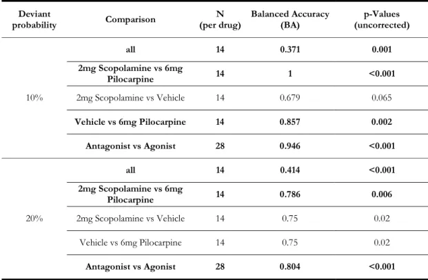
5.9.2 Results Part 1: 20% Deviant Probability (MMN_0.2) ... 149

5.9.4 Results Part 3: Constraining Parameters across Pharmacological Conditions

... 158

5.9.5 Discussion ... 163

6| Effective connectivity during a self-calibrating visuo-spatial working memory paradigm ... 169

6.1 Disclaimer ... 169

6.2 Abstract ... 171

6.3 Introduction ... 172

6.4 Methods ... 175

General Information ... 175

Task Design ... 175

Behavioral Data Analysis ... 177

Functional Data Acquisition & Preprocessing ... 178

Subject Level Modeling ... 178

Group Level Modeling ... 179

Dynamic Causal Modeling ... 180

Regions of Interest and Time Series Extraction ... 181

Model Space ... 181

Bayesian Model Selection and Bayesian Model Averaging ... 182

6.5 Results ... 183

6.5.1 Behavioral Results ... 183

6.5.2 Group-Level GLM Results ... 183

6.5.3 Dynamic Causal Modeling ... 185

6.6 Discussion ... 189

6.7 Supplementary Material ... 194

6.7.1 Assessment of Time Series Extraction ... 194

6.7.2 Dynamic Causal Modeling ... 194

7.1 The Story so far ... 199

7.2 The Story to come ... 204

Appendix A| Analysis Plan for the RATMPI study ... 207

Appendix B| Analysis Plan for the PRSSI study ... 225

References ... 239

Equation Section 1

1| INTRODUCTION

1.1 THE MOTIVATION

Computational Psychiatry (CP) is a young field that emerged in the early 2000s, bringing the application of computational theories and mathematics into the realm of psychiatry. It is part of a larger family of disciplines embedded under the umbrella term of ‘computational neuroscience’ (Frässle, Yao et al. 2018). While ‘computational neuroscience’ generally aims at describing how the brain processes information, CP’s goal is to develop and test mathematical models of the brain or behavior, to address and solve explicit clinical problems. One of the clinical problems in psychiatry is that the current symptom based nosology is successful in broadly stratifying patients into subgroups, yet these subgroups contain little predictive information about treatment success or disease trajectory. In a nutshell, psychiatry lacks a predictive ‘biomarker’ (Kapur, Phillips et al. 2012). CP tries to bridge this gap. The term ‘computational’ here has a double meaning. On one hand, CP sees the brain as an organ that performs computations in order to process information. As a biological system however, it is bounded by certain constraints such as availability of pathways and messengers that allow for the communication between brain areas. These areas are thought to have important functions for the interpretation of the information.

This has been formalized by seeing the brain as an inference machine that creates a predictive, learning model of the world in order to minimize surprise about new, sensory stimulation (Friston, Kilner et al. 2006). However, if any of the previously mentioned (biological) resources are ‘malfunctioning’, this could lead to aberrant models of the world,

aberrant model-adjustments and in turn constant “surprise”¹. As a consequence, constant surprise causes a lot of stress (as it would on any organ). (Mal-) Adaptation to this stress might result in pathological beliefs and/or behavior.

On the other hand, ‘computational’ also refers to the tools CP uses in order to understand this problem. It tries to build and formalize simplified, mathematical models of the mechanisms underlying cognition, behavior or physiology and their possible perturbation in psychiatric disorders (Frässle, Yao et al. 2018). In other words, its main goal is to use computational tools to gain an aetiological understanding of psychiatric diseases, moving away from a purely symptom based description. This new level of description of disease processes holds promise to yield more credible predictions of clinical trajectory and allow for differential treatment (e.g. (Montague, Dolan et al. 2012, Stephan and Mathys 2014, Wang and Krystal 2014, Huys, Maia et al. 2016)).

One of the most prominent examples of such a description of putative disease processes is the ‘dysconnection hypothesis’² that has been formulated in the context of schizophrenia.

It postulates aberrant interaction between NMDA³ receptor (NMDAR) dependent plasticity and neuromodulators (NNI) (Friston 1998, Stephan, Baldeweg et al. 2006, Stephan, Friston et al. 2009). According to this theory, the spectrum nature of schizophrenia is a consequence of the variable ways in which genetic-environmental influences can alter NNI, resulting in tremendous variability of clinical trajectories and treatment responses across patients.

Despite clearly formulated hypotheses, CP has yet to deliver a proof of its clinical utility.

There are multiple reasons. First, as shown in the example of schizophrenia, the stated hypotheses are inherently a highly multivariate problem. Second, medication affecting different neurotransmitter systems have shown efficacy for certain psychiatric diseases.

However, it is unclear why or how exactly they work in the brain as medication is typically applied systemically. Third, connected to this, positron emission tomography (PET) is the only non-invasive brain imaging technique to investigate neurotransmitter systems directly;

yet, requires the injection of a positron-emitting radioligand.

1 Here, surprise is meant metaphorically. However, ‘surprise’ also has a mathematical meaning which is part of many models

2 The hypothesis was originally named ‘disconnection’ before being refined into ‘dysconnection’.

3 N-methyl-D-aspartate receptor (NDMAR)

Figure 1| Schematic overview of the generative embedding approach; Mathematical models used to infer on hidden neuronal processes. Patient stratification based on inferred parameter estimates or model selection. Overview in line with (Brodersen, Deserno et al. 2014, Frässle, Yao et al. 2018). Parts of the Figure courtesy of Sara Tomiello.

A possible way to address the investigation of neuromodulatory action using other methods was suggested in the context of modeling brain physiology and connectivity. Here, specific cognitive tasks⁴ are used, where evidence for involvement of particular neurotransmitters has been demonstrated. These tasks are combined with non-invasive neuroimaging techniques (electroencephalography (EEG), functional magnetic resonance imaging (fMRI)), eye-tracking or other physiological readouts. The measures of neural activity (or other measures) are then thought to convey information about the neuromodulatory processes (e.g. (Aponte, Schöbi et al. 2019), for review, see (Iglesias, Tomiello et al. 2017, Heinzle and Stephan 2018)). The last step to gain an aetiological understanding of disease mechanisms, is to model this task-based (or unconstrained) activity by means of a dynamical system model. CP then argues that it is at the level of models (or their parameters) where pathophysiologies are encoded. The hypothesis is that patients separate into subgroups based on these models and/or model parameters, for example with respect to treatment.

This differentiation can be formulated as a statistical problem of comparing parameter estimates or distributions, or by encoding different hypotheses in different model architectures (Frässle, Yao et al. 2018). The procedures described here have been termed

4 or unconstrained cognition

‘Generative Embedding’ (Brodersen, Deserno et al. 2014) and show a clear analogy with what is known in medicine as differential diagnosis.

Two tasks that have robustly shown sensitivity and specificity to neuromodulatory influences are the mismatch-negativity (MMN) and working memory (WM) paradigm (Iglesias, Tomiello et al. 2017). Furthermore, both paradigms have been shown to be clinically relevant for schizophrenia as elicited neural responses differ between healthy controls and patients (e.g. (Roth, Pfefferbaum et al. 1981, Park and Gooding 2014)).

However, the two tasks are assumed to involve very different neurotransmitter systems. In brief, the MMN refers to characteristic differences in the evoked response potentials (ERPs) to attended and un-attended stimuli. It was suggested that it reflects a prediction error signal updating an internal model of the world. Hence it could resemble learning.

While it has been shown that the MMN can be manipulated with drugs affecting the cholinergic transmitter system (Moran, Campo et al. 2013), it seems that dopamine is less involved (Leung, Croft et al. 2009). Dopamine on the other hand has been associated with WM (Sawaguchi and Goldman-Rakic 1991). WM denotes a special type of memory storage with ability to retain and manipulate limited amounts of information over short periods of time (D'Esposito and Postle 2015). Importantly, NMDAR function is expected to be crucial in the generation of persistent activation over time due to their longer time constants.

Therefore, WM is an interesting testbed to infer on NMDAR function and potential modulation thereof by dopamine (Durstewitz and Seamans 2002). The empirical studies presented in this thesis focus in more detail on these two tasks.

The mathematical modeling of these task-based data asks for a very special type of models that respect both the nature of the latent (hidden) processes on the neuronal level and the resolution of the imaging technique. One such method, dynamic causal modeling (DCM), was formulated in the early 2000s for fMRI (Friston, Harrison et al. 2003). It models the effective (directed) connectivity between brain regions. The way neuromodulatory action here can be understood is in the enhancement or reduction of connection strengths mediated by neuromodulators. Not much later, DCM were adapted to be used for electrophysiological data (David, Kiebel et al. 2006). Because of the much higher temporal resolution of EEG, synaptic action can be directly incorporated in the models.

Critically, in order for DCMs (and, in fact, any model) to become truly useful for CP, the robustness and reproducibility of these tools is paramount. This is because in CP, reproducibility, generalizability and stability of model based approaches have direct

consequences on acceptance (in order to achieve actual, clinical implementation) of the new methods into everyday clinical practice and, ultimately, on patient well-being. This is even more critical given the remarkable complexity of these models and the computational challenges that are associated with that. Despite the importance of the robustness of the approach, so far only little work has been done on systematically testing the robustness of DCMs in a standard setting where it is typically applied to data. Notably, this scenario is by no means exclusive to DCM, but can be observed for a wide range of computational modeling approaches in all fields of science. For instance, according to Henderson et al.

(2018), over 10’000 reinforcement learning (RL) related papers have been published yearly between 2012 and 2016 (Henderson, Islam et al. 2018), with those papers displaying a large variability in the exact (deep) RL methods used and the way results are reported. The authors conclude that as a consequence, results and indicated improvements by the respective methods do not easily generalize and that there is an overall lack of homogeneity.

On a broader scheme, this critique is ubiquitous across all scientific disciplines as revealed by a current search on google scholar using the terms ‘reproducibility, crisis, science’ yielding over 10’000 results since 2018.

To address this shortcoming in the context of DCM, the goal of this thesis is to conduct a systematic investigation of the robustness of the method and provide a more thorough understanding of potential challenges, as well as to develop practical solutions and recommendations that address these issues when applying these models to real-world data.

In this context, it is useful to briefly emphasize some important characteristics of the models utilized here (i.e., DCMs) – and to point out some important differences compared to classical machine learning (ML) models. First, they are biophysically interpretable models as they grounded in our current knowledge about fundamental physiological processes.

Consequently, their parameter estimates promise to convey information about neurophysiology and the data generating processes. Second, the models used in CP are applied to reduce the complexity of the problem and to, potentially, facilitate a mechanistic understanding. While classical ML algorithms can be very good at prediction, they typically operate in orders of magnitude higher dimensional parameter spaces and would provide little to no systematic understanding of a disease. Third, all models we will present are so called generative models which follow Bayesian statistics. That is, the parameters of the models are considered random variables, while data is fixed. Importantly, parameters ( )

are assigned a priori probabilities (prior distributions ^{p( )} ) and the posterior belief about parameters, conditioned on the data (y), follows Bayes’ Rule

( | ) ( )

| ) ( )

( .

p p y p

y p y

 

  ^ (1.1)

There is a lot of debate on the function and specification of prior distributions, and generally between the Bayesian approach and the frequentist counterpart. When I took a course on Bayesian statistics in 2017, the lecturer’s response to the dispute was (and I am paraphrasing):

“… it is not about superiority of Bayesian over frequentist statistics. It is about understanding their relationship, making sensible choices and trying to get the best out of both worlds. “

I think this view is very useful and much of this thesis is devoted to getting a quantitative understanding of the overarching theoretical framework that is paving the way towards using models as computational assays for differential diagnosis, and their explicit implications for DCMs. Regardless of whether the models are Bayesian or not, the idea for them to provide physiologically interpretable meaning comes at a cost. Face, construct and predictive validity pose additional demands on them to be truly able to achieve their goal.

All models are subject to decisions of the modeler that might affect all three previous demands (e.g. prior distributions). As we will see, there are other crucial factors that challenge construct validity, robustness and reproducibility. These include assumptions about the independence of datapoints, correlations between parameters, assumptions about the irreducible variance in the data and, very often, small sample sizes.

1.2 THE STORYLINE

In this dissertation, we address the problems laid out above by first considering theoretical and computational aspects of the modeling and model inversion and then applying these new developments in the context of two experimental datasets.

In Chapter 2, we look at the integration of delay differential equations underlying DCM for EEG. Including delays between different neuronal populations assures that the model respects the physiologically known conductance delays between cortical regions, which cannot be neglected given the high sampling rate of EEG. The delays can change a system’s

dynamic repertoire. The cost of this strive for realism is that delay differential equations are much more difficult to integrate compared to their non-delayed counterpart. The first part of the methodological section benchmarks the current integration scheme for these models against two, in-house developed variants and a state of the art scheme (based on a Runge- Kutta scheme) in a number of simple systems. We show that the default implementation violates construct validity both in terms of causality and dynamics, whereas they appear to be respected in our alternative procedures. While accuracy is arguably the most important criterion for assessing the performance of the integration schemes, computational efficiency is a critical factor as well.

In Chapter 3, we investigate the problem of optimization in DCMs. Already in 2011, Daunizeau and colleagues mentioned some critical aspects of the statistical inference techniques (Daunizeau, David et al. 2011). Some of these points have been investigated, but often at the cost of much more computationally costly methods (Penny and Sengupta 2016, Sengupta, Friston et al. 2016)⁵. Most crucially, network identification and parameter estimations hinge on an optimal (in a Bayesian sense) computation of the posterior distribution. It itself however, depends on the optimization landscape (we will derive the dependency in the chapter). For non-convex optimization problems, the local optimization routine based on a gradient ascent routinely implemented in DCM is not guaranteed to find the globally optimal solution. If inversions end in a local optimum, objective model assessment criteria derived from Bayesian theory therefore might not be applicable. Local extrema also pose replicability problems, as results will depend on particular starting values of the optimization and local gradients. In this second part, we demonstrate that the objective function (the negative free energy) for the case of our simulations does present with critical structures which, from the algorithm’s perspective are identified as local optima. To account for this problem, we augment the standard inversion approach by starting multiple inversions in parallel from different starting values. They allow us to diagnose and quantify the problem of local optima both in terms of resulting posterior distributions and the score of model goodness. We assess model and parameter recovery and compare as to what degree conclusions drawn are dependent on the starting values.

The presented augmentation of the inversion helps to overcome some of the caveats, while it remains easy to implement, building on the same (default) optimization framework. But it also illustrates that further constraints are needed, if meaningful homogeneity in

5 Unfortunately, to our best of knowledge, these works have not been followed up.

parameter estimates and comparability of effects need to be achieved across studies in the future. Our results also provide a possible explanation for why studies may find seemingly conflicting results if standard procedures are used.

In Chapter 4 we focus on the criteria of model goodness. We derive approximate relationships between a measure of model goodness that can be interpreted in absolute values, i.e. residual sum of squares and an objective Bayesian measure of model goodness, the negative free energy. These relationships provide an explanation for many surprising quantitative findings in the literature. First, they explain why empirical evidence favoring one model over another can vastly exceed the standard thresholds. Second, they illustrate how false assumptions about the (in-) dependence of residuals can cause tendencies to overfit and bias towards complex models. Third, they illustrate that hyperprior specification deserves special care, as misspecification can lead to biased inference on models simply driven by these a priori assumptions. The conclusion from these findings will be the following: While one can argue that inference is always dependent on modelling assumptions, our results demonstrate that the field should be aware of the severe consequences some of them might have in practice and, if possible, agree on standards in terms of data-preprocessing, model assumptions etc. in order to make results comparable across studies and robust for single patient predictions.

These three chapters conclude the theoretical and model development part of this thesis.

The software for the integration scheme, the augmentation and diagnostics of the inversion procedure and the diagnostics of hyperparameter optimization will be made publicly available in the in-house developed, open source software collection TAPAS (https://www.tnu.ethz.ch/en/software/tapas.html).

The second contribution of this thesis is the application of these models to empirical data, both in EEG and fMRI, capitalizing on the lessons we learned in the first part of this thesis and the developed improvements of the DCM machinery. As highlighted above, the empirical analyses will concern MMN and working memory paradigms, and thus have a strong link to neuromodulatory processes and clinical questions.

In Chapter 5, we first show the application of DCM for electrophysiological measures. We use DCM for evoked response potentials (ERPs) to infer on graded, muscarinic changes of effective connectivity in rodents in an MMN paradigm. Here, we make explicit use of the first two methodological advances and show that DCM can successfully reduce the number of features by a factor of 50. The ensuing parameter estimates not only have physiological

interpretation, but also selectively convey information about the pharmacological setting.

Throughout this thesis, we will refer to this study as RATMPI.

The second empirical contribution (Chapter 6) is the application of DCM for fMRI in a working memory paradigm. The paradigm was developed during this PhD and allows for online titration of task difficulty – a crucial confound when it comes to bringing WM to a clinical setting. Here, we will make use of the methodological developments two and three, and propose a way how informed hyperpriors can be specified in DCM for fMRI. We will refer to this study as PRSSI.

The final Chapter 7 of this thesis will provide a discussion that connects the findings of the methodological and data analysis chapters and provides an outlook.

Notably, the work presented in this thesis (and briefly outlined above) represent only a selection of the projects I contributed to over the course of my PhD. In particular, I was further involved in two additional studies. First, I was the main contributor to an EEG study with 162 healthy controls, where participants performed the mentioned Working Memory task under pharmacological intervention. In a double blind, placebo-controlled, between subject design, participants underwent a cholinergic or dopaminergic intervention with either agonistic or antagonistic effect. Second, I was main contributor in a longitudinal patient study with patients suffering from psychotic symptoms. Here, the goal will eventually be to predict the success of a treatment switch from a non-cholinergic to a cholinergic anti-psychotic, based on WM EEG data. The analysis of these datasets is subject to future work, and lies beyond the scope of this dissertation.

In the rest of this introduction, we will provide a brief introduction the generative model of DCM and how hypotheses can be tested in a Bayesian framework. They will later be used for reference. We here focus on DCM for ERP since these represent the main workhorse utilized in this thesis. The present summary is thought as a concise summary of the mathematical literature associated to DCM for ERP and we refer to the original work (David, Kiebel et al. 2006) or this review paper on the mathematical machinery (Ostwald and Starke 2016) for an in-depth treatment of DCM for ERPs. Furthermore, a comprehensive treatment of model comparison in DCMs can be found in (Penny 2012).

1.3 INTRODUCTION TO DYNAMIC CAUSAL MODELING FOR ERP

1.3.1 A

DCM for ERP assumes that the data measured in EEG is generated by neural activity in one or multiple connected cortical columns. Each column typically comprises three different kinds of cell populations: excitatory interneurons (stellate cells), inhibitory interneurons (inhibitory cells) and (excitatory) pyramidal neurons (pyramidal cells)⁶. Populations can be understood as modeling population dynamics, i.e. postsynaptic potential (probability-) distributions over a population of single cells. If the distribution activity is simplified and only described by its mean, one is operating in the Neural Mass approximation. In the following, we will always use this assumption. Populations within a cortical column are connected via intrinsic connections. Between columns, populations are extrinsically connected. Extrinsic connections show a well-defined layer specificity which distinguishes forward and backward connections in the cortical hierarchy based on the seminal work by (Van Essen, Anderson et al. 1992). Figure 2 illustrates a simple neural mass model which dates back to the work of (Jansen and Rit 1995). This allows for modeling processes along cortical hierarchies, which is fundamental to test hypotheses about information-processing and learning.

6 Over the years, multiple variants of DCM for EEG have been formulated. In light of the relevance for this thesis, we limit our discussion to the original convolutions based version, including three subpopulations David, O., S. J. Kiebel, L. M. Harrison, J. Mattout, J. M. Kilner and K. J. Friston (2006). "Dynamic causal modeling of evoked responses in EEG and MEG." Neuroimage 30(4): 1255-1272.. We used this variant for most of the methodological developments. In the empirical RATMPI study, we used a different architecture of the single, cortical column; the so called Canonical Microcircuit (CMC, Bastos, A. M., W. M. Usrey, R. A.

Adams, G. R. Mangun, P. Fries and K. J. Friston (2012). "Canonical microcircuits for predictive coding."

Neuron 76(4): 695-711.). The details of this circuit will be explained in the corresponding chapter.

Figure 2| Schematic overview of a single cortical column. Architecture based on the original, three population model. Outgoing connections (to other columns) always originate from the pyramidal cell. Both, interneurons and pyramidal cells are thought to populate supra-granular layer II/III and infra-granular layer V.

1.3.2 N

M

There are two fundamental mathematical operations that give rise to the generic equations underlying the convolution based DCM formalism and hence the neuronal dynamics. First, average post-synaptic population potentials are being modeled. They are thought to arise from average incoming activity of other populations. This average is formulated as a convolution () between a parametrized convolution kernel (H) and the incoming firing of another populations (). The convolution kernel here describes a cell-specific property of how unit-firing changes the post-synaptic potential, parametrized by a gain h and a (inverse) decay parameter . Hence, one could think of it as a summary of all channel properties onto one population. Second, average post-synaptic potentials lead to average cell-firing at time t, i.e.  ( ( ))v t . This is formulated via a sigmoid-transformation (Jansen and Rit 1995). For a single cell subject to incoming firing, the post-synaptic potential is described by

( ) ( ) ( )

( ) ex 0

)

p( )

( ( )

,

v t t H t d

H t h t t

t H t

t

    

 

  

   







 



We now derive the general form of the equations by taking the derivative wrt. t:

( )

( )

( ) (0) ( ) ( ) ( )

( ) ( )

t t

t t

v t h t H e d v t

H e d v t

 

 

     

    

 



 



   

  







(1.3)

where we made use of the Leibniz rule in the first step, and the fact that h(0) 0 . Taking the second order derivative yields

( ) 2 ( )

2 ( )

( ) ( ) ( )

( ) ( ) ( ) .

( ) ^{t t t t}

t t

e

H t H e d v t d

t H d v

v

d t

H e t

  

 

       

      

   



 





 

 







 



(1.4)

Multiplying Eq. (1.3) with  yields

2 (^t ) ( ) ( ) 2 ( ).

t H e^{ }    d v t  v t

  



which can be inserted in Eq. (1.4) to result in the 2^nd order differential equation underlying the convolution based DCMs:

( ) 2 ( ) 2 ( ).

( )t t v t

v H    vt

 ^(1.6)

Note that this equation is equivalent to the dynamic equations of a driven, critically dampened, harmonic oscillator. Eq. (1.6) describes the average, post-synaptic potential of a single population of cells for a single, arbitrary input ( )t . For multiple inputs, this can be trivially extended to

1

( 2

( ) 2

( ) ⁿ ) _j ( ).

l l lj l

j lj j lj j l i

v t H   t  v t  v t



 

   





  ^(1.7)

Here, we already index that we have selected an arbitrary population (l) that is connected to multiple other populations ( j). The connections here are encoded by an indicator matrix

lj, which is  _lj 1 if two populations are connected and  _lj 0 otherwise. This matrix can be directly read out from the connectivity pattern in Figure 2. Here, we basically state that each connection is modeled through its own kernel (i.e. channel properties), parametrized by the kernel gain Hlj and inverse kernel decay lj. However, a general problem of all models is to somehow evoke parameter constraints. Otherwise, there are simply too many inherent correlations and parameters cannot be estimated without large uncertainties in the estimates. For example, for the intrisic connectivity pattern of a single

cortical column shown in Figure 2, without constraint, the connection specific kernels would already amount to eight parameters per cortical column.

Therefore, usually three simplifying assumptions are made:

 (inverse) kernel decays  are region and effect specific (whether a connection is excitatory (^e) or inhibitory (i)):

/, {1,2,..., }

e i

lj r r R

  

 kernel gains H are region, effect and connection specific

/ /

, for extrinsic connections for intrinsic connections ,

e i

r lj

lj e i

r lj

H H H

A



 

 

This brings the notion of connections strengths A_ij,_ij which are factors enhancing or depleting the region specific baseline gain.

 The intrinsic connection strengths _ij are fixed across regions, i.e. specific intrinsic connections between the same populations have the same strength across regions

, {1,2,3,4}.

ij p p

  

Together, these simplifications result in the postsynaptic potential population i in region r to obey the following differential equation:

/ 1

/ / 2 /

( ) ( ) ( ) 2 ( ) ( ).

r

n r

e i e i e i e i

l r lj lj j r l r l

j

t

v t H  A    v t  v t



 

 

 





  ^(1.8)

Here, the indicator-matrix  is absorbed directly in the variables A and . Under these assumptions and considering for example four cortical columns, the number of synaptic parameters over the two cortical columns are 20 instead of 32 (not taking into account extrinsic connections).

For the system described in Eq. (1.8), initial conditions of v t(  0) 0is a fixed point, hence the system will always stay at rest. An external, driving stimulus then perturbs the system away from this equilibrium position. Typically, one assumes that it is some pulse shaped, thalamic input u caused by some external stimulation (e.g. a brief tone). With the arguments so far, this can be directly added in Eq. (1.8).

/ / / 2 / 1

)

( ) ^{n e i} _r^{e i} ( _lj) ( _{l l}( ) 2 _r^{e i} _l( ) _r^{e i} ( ).

rl r j l

j lj

v t H  A   t Cu t  v t  v t



 

 

  

 





  ^(1.9)

External stimulations are always thought to excite the populations in the granular layer IV as can be read out from the connectivity pattern in Figure 2. Therefore, C_l0 if l does not correspond to the index of a stellate cell. Moreover, there might be multiple different inputs driving the system, and we therefore also index u. An alternative interpretation would be to consider ^u as an additional, non-interacting state whose output does not undergo a sigmoid transformation. This would be congruent with Eq. (1.9) and gives it the same notion of some un-observable (thalamic) state, with C enhancing/depleting the baseline synaptic gain, equal to the interpretation of A and .

Finally, we allow that one population might exert its effect over another population with some temporal delay  . In other words, the post-synaptic potential changes with respect to some earlier, average firing, hence

/ 1

/ / 2 /

( ) ^{n e i} _r^ei ( _lj) ( _l) _{l l}( ) 2 _r^{e i} _l( ) ^{e i} _l( ).

rl r lj j r

j j

v t H  A   t  C u t  v t  v t

  

    

  

 





  ^(1.10)

These delays render the ordinary differential equations in Eq. (1.9) to become delay differential equations (Eq. (1.10)), which has some important implications on how the system needs to be integrated. We will leave this point for the respective Chapter 2. As mentioned in the footnote, there are other assumptions or constraints that one could make on the system, which will give rise to other variants of the model. Here, we merely aimed at outlining the origin of the equations for the convolution based DCM, based on the ERP architecture with three subpopulations, as implemented in Statistical Parametric Mapping (SPM12, ver. 6906) software package (www.fil.ion.ucl.ac.uk/spm).

In the literature, state variables (here v t( )) are often referred to as x and Eq. (1.10) is expanded into a system of 1^st order differential equations. If we denote

2 / 1

/ / 2

1

/

1( ) ( ) ( ) 1

) ( ) ( )

1,.

) .

( ) (

,2 )

( (

.

2

l

n

l r r

l

e i e i e i e i

l r lj lj j lj l l r

j l l

t H A t x t x t

l n

x t x t

x t x    t  C u  





 



 

       



 

 



  (1.11)

the set of differential equations in Eq. (1.11) is of order 1, but models the same dynamics as Eq. (1.10). Here, ⁿ denotes the total number of populations (across all cortical columns).

From the perspective of electrical circuits, the auxiliary states can be interpreted as currents flowing through the cell membrane (the change of voltage of a capacitor equals the current).

It should be noted that the actual implementation extends the states associated to pyramidal cells into hyper- and depolarizing states. However, for our brief review, we will not go into this level of detail.

1.3.3 F

M

In order to derive a full generative model that can generate EEG data, a forward mapping from latent states described by the dynamical system above to observed variables is necessary. This is needed to assign the likelihood of the data, given the prediction and parameters. We will see in Chapter 3, how this can then be turned into an objective function that trades off accuracy and complexity with respect to which parameters are optimized.

For electrophysiological data, the observed data lives either in the space of principal components of scalp potentials, or epidural/local field potentials (LFP). For simplicity, we will focus on the latter, also because in this thesis, no scalp data was analyzed but only LFPs.

In this case, the number of channels (n_c) matches the number of cortical columns. We assume that the measured LFP potentials (measured in the unit of volts [V]) come from a linear mixture of the average post-synaptic population potentials. Put simply

2

) ( )

(

c p

n p

n pst pst

y x t

t pst

y M

M t

x G













 ^(1.12)

where we explicitly indicate that both, the predicted data y_p and the hidden states x are matrices. Here, x t( ) are the integrated states over peri-stimulus time (pst) of Eq. (1.11).

Hence, ^G is a matrix, mapping from the latent states to the predicted observation:

2 nc n

G M ^ . There are some constraints on the entries of this so-called lead field matrix ^G:

 Only voltage states (x_i in Eq. (1.11)) contribute to the LFP potentials

 There is no mixture between the voltage of a single cortical columns and other channels

 Each population exerts equal gain J_P (across cortical columns)

 Each cortical column (i) exerts a region (i) specific gain Li (equal across populations of this column)

Collectively, this amounts to

0 for not being a voltage state

0 for not being a voltage state not associated with channel for being the post-synaptic potential of a population in column

ij

i p

j

j i

J j p i

G L



  

(1.13)

In this mathematical formulation (depending on how the states are exactly concatenated), G has a block-diagonal form.

1.3.4 I

S

In order to make DCM more accessible, we have created a didactic, interactive visualization tool (Figure 3). It allows to dynamically change parameters and visualizes changes in the predicted responses at the hidden neuronal level and changes in the observed responses. It is MATLAB based, ties into the existing functionality of SPM, and will be released in one of the upcoming TAPAS releases in 2020.

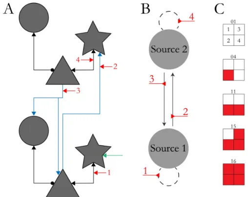
Figure 3| Interactive user-interface for the simulation of signals in the convolution based DCM for ERP framework. A) Interactively change parameter setting to visualize changes in the signal. B) Responses of the neuronal populations for the current parameter set. C) Responses of the neuronal populations for the previous parameter set. D) Convolution kernel for the current and previous parameter set. E) Driving Input for the current and previous parameter set. F) Toggle to display only a subset of populations. G) Toggle to activate the ‘observed-responses-panel’ (right panel). H) observed responses for the current and previous parameter set.

1.3.5 G

M

The generative model then entails the probabilistic information about the data-generating process under assumption of noise. We assign a Gaussian likelihood to datapoints that is, the probability of a time-series y given a prediction y_p plus some error, which we assume to be distributed according to a Gaussian with some parametrized error covariance ( )_h , is given by

.

| (0, ( ))_h

y ypN  (1.14)

We will go in detail into this part in Chapter 3. Hence, the full joint probability of data and parameters can be written as

, , ) ( | , ) ) ( )

( ( ) ( ) | ( )) ( ) ( ) ( ).

( , _{h g p h g}, _p) ( _h ( _p

g p h h

g

g p

p p y p

N y G x p p p

y      p p 

     

   

       ^(1.15)

For completeness, we have written down all dependencies of the variables in Eq. (1.15).N denotes a multivariate normal distribution. We assume a priori independence between the parameter classes, i.e. neuronal parameters (_p{ ,H , , , , }C A ), parameters of the forward model (_g{ , }L J ) and hyperparameters of the noise model (h). This notion of the parameter classes and the notation will be used throughout the methodological part of this thesis.

1.4 MODEL EVIDENCE AND MODEL COMPARISON

In a Bayesian setting, the goodness of a model m can be understood in terms of the model evidence or the marginal likelihood of the data y under the prior p( | ) m ⁷:

. ,

( | ) ( | m) ( | )

p y m 



Put simply, it denotes the likelihood of the observed data under the prior. Comparing two competing models in a Bayesian setting amounts to computing the ratio over model evidences (or the difference in log-model evidences):

7 Note that in our notation, we indicate explicitly that the parameters  come from model m. Alternatively, one could write p y( |_m)or just omit the index and keep the dependency in mind.

12 1

2

12 1 2

|

log ( | ) log ( | ).

( | )

( )

log

p y m

B p

B

m

p y m p y

y

 m





(1.17)

These quantities are known as Bayes’ Factor and Log Bayes’ Factor (Kass and Raftery 1995).

This can be seen as a Bayesian way of hypothesis testing. For example, in the context of DCM, m1 and m2 could encode different hypotheses about how the network changes under some perturbing stimulation. To draw the link to the empirical studies presented in this thesis, these ‘perturbations’ or ‘condition specific effects’ could either be the presentation of an unexpected tone (MMN) or the need to retain information in working memory (WM). Importantly, Kass and Raftery (based on (Jeffreys 1961)) also provided guidelines on interpreting the Bayes’ Factor in a quantitative manner. According to those, a Bayes’ Factor of

12

log 12 3 20 B B 



speak for strong evidence in favor of m₁ over m₂ (Kass and Raftery 1995). The log of the quantity in Eq. (1.16) (the log model evidence, LME) has an interesting property:

) log ( ) log ( ) (

( | ) (

log (

(

| )

) | )

|

( | )

log ( | ) ( | log ( | ) .

( )

Accuracy )

Complexity

y d y d

p y

p y p y d

p y p y p

p y p p

p y d y

p p

 

   



     





 









 



(1.18)

Accuracy is the expected log-likelihood of the data under the posterior. Complexity is the Kullback-Leibler-Divergence between the posterior and prior distribution, and a measure of similarity. By definition, it is positive (semi-) definite and only equal to zero if the two distributions are identical. Therefore, it can be seen as penalizing overly complex models and formalizes the principle of Occam’s razor (Beal 2003, Penny 2012). This property becomes important when comparing two models. Specifically, the decision which of two models provides a better explanation for the data depends not only on how well it predicts the data, but rather on a full accuracy-complexity-tradeoff.

Obviously, the tradeoff hinges on the correct computation of the model evidence. As we will see, this is a computationally challenging problem, as computing the integral in Eq.

(1.16) is usually not feasible. In Chapter 3, we will show that one can approximate the LME and turn the problem of computing it into a problem of optimization. This optimization not only returns a value for the model goodness, but also an approximation to the posterior distribution of the parameters.

This concludes the introduction to Dynamic Causal Modeling for ERPs and the introduction to this dissertation.

Equation Section 2

2| INTEGRATION OF DELAY DIFFERENTIAL EQUATIONS

2.1 DECLARATION

These methodological developments and analyses were done under the supervision of Jakob Heinzle and Klaas Enno Stephan. Data collection for the empirical analysis was done by the Max-Planck Institute in Cologne by Fabienne Jung as part of the doctoral thesis.

This dataset was previously used in a publication (Jung, Stephan et al. 2013). For more information on the dataset, we refer to Chapter 5.

2.2 INTRODUCTION

In DCM for EEG, neural dynamics are described in terms of delay differential equations (DDEs, see Eq. (1.11)). Delays refer to temporally delayed effects one population exerts over another. In the convolution based DCM framework, delays come in two flavors – extrinsic and intrinsic delays, which however are merely associated with differences in the a priori expectation of their magnitude. They both describe delays between the output of a population, i.e. the sigmoid transformed post-synaptic potentials and the receiving (input) population. These directed dependencies are easily accessible when looking at the full connectivity pattern of a network (see Figure 2). The biophysical reason for delays is simple – action potentials travel at a finite velocity through axons, with large variation in speed depending on multiple factors (e.g. myelination or axon diameter). Reported velocities range from 0.1 up to 120 m per second (Swadlow and Waxman 2012). For cortico-cortical

connections (which are most relevant for EEG), animal studies have reported delays between 0.5 ms and 42 ms⁸ (Miller 1975, Swadlow 1990, Ferraina, Paré et al. 2002), but considering relays of activity through non-modelled sources, one could also think of longer delays, especially, since axonal connections in humans tend to be longer.

Delays render ordinary differential equations (ODEs) to become delay differential equations (DDEs). We will not go into too much detail about the general application of delay differential equations, and reduce the general overview to the relevant features for the discussion of this chapter. The following overview constitutes a brief summary of chapters 1-3 of a basic text book on “Numerical methods for delay differential equations” (Bellen and Zennaro 2013).

In general, 1^st order ODEs are characterized by the following set of equations

0

0 0

( ) ( , ( )), ( )

x t f t x t t t tf

x t x

  





where 𝑥 denotes the state variable or state, 𝑡 denotes time, 𝑡 and 𝑡 the initial and end timepoint and 𝑥 the initial value (hence, also the commonly used term initial value problem).

The step to DDEs then includes dependencies of the previous equation on past values of 𝑥

0 0

( ) ( , ( )), ( ) ( ),

x t f t x t t t tf

x t t t t





   

 

 (2.1)

with 𝜏 ∈ [−𝑟, 0], 𝑟 ∈ [0, ∞) now being semi-positive delays, and 𝜙 an initial state function.

This initial state function renders the solution un-smooth at the transition point, as there (generally) is a jump in the derivative. Such a discontinuity propagates throughout the integration interval, and as a consequence, 𝑥(𝑡) is only 𝐶 −continuous on the interval [𝑡 , 𝑡 ] (Bellen and Zennaro 2013).

In the first chapter of their book, (Bellen and Zennaro 2013) provide a number of examples illustrating implications for the behavior of a system when introducing delays. Most prominently, delays can stabilize or destabilize a system, can lead to non-uniqueness of solutions, exhibit oscillatory or chaotic behavior, etc. when compared to the sibling ODE

8 Delays up to 42 ms is arguably long, even for humans. Miller et. al (1975) do report such a latency in cat cortex, but most of the mass in the histogram is around 10-20 ms.