Contents lists available atScienceDirect
Journal of Marine Systems
journal homepage:www.elsevier.com/locate/jmarsys
Iron organic speciation during the LOHAFEX experiment: Iron ligands release under biomass control by copepod grazing
Luis M. Laglera
a,b,⁎, A. Tovar-Sanchez
c, C.F. Sukekava
a, H. Naik
d, S.W.A. Naqvi
d, D.A. Wolf-Gladrow
eaFI-TRACE, Departamento de Química, Universidad de las Islas Baleares, Palma, Balearic Islands 07122, Spain
bLaboratori Interdisciplinar sobre Canvi Climátic. Universidad de las Islas Baleares, Palma, Balearic Islands 07122, Spain
cDepartment of Ecology and Coastal Management, Andalusian Institute for Marine Science, ICMAN (CSIC), Campus Universitario Río San Pedro, Puerto Real, Cádiz, Spain
dNational Institute of Oceanography, Dona Paula, Goa, India
eAlfred-Wegener-Institut Helmholtz Zentrum für Polar- und Meeresforschung, Am Handelshafen 12, 27570 Bremerhaven, Germany
A R T I C L E I N F O Keywords:
LOHAFEX Iron cycling Iron speciation Grazing Southern Ocean Iron fertilization
A B S T R A C T
The LOHAFEX iron fertilization experiment consisted in the fertilization of the closed core of a cyclonic eddy located south of the Antarctic Polar Front in the Atlantic sector of the Southern Ocean. This eddy was char- acterized by high nitrate and low silicate concentrations. Despite a 2.5 fold increase of the chlorophyll-a (Chl-a) concentrations, the composition of the biological community did not change. Phytoplankton biomass was mostly formed by small autotrophic flagellates whereas zooplankton biomass was mostly comprised by the large co- pepodCalanus simillimus. Efficient recycling of copepod fecal pellets (the main component of the downward flux of organic matter) in the upper 100–150 m of the water column prevented any significant deep export of par- ticulate organic carbon (POC).
Before fertilization, dissolved iron (DFe) concentrations in the upper 200 m were low, but not depleted, at
~0.2 nM. High DFe concentrations appeared scattered from day 14 onwards as a result of the grazing activity. A second fertilization on day 21 had no significant effect on the DFe and Chl-a standing stocks. Work with un- filtered samples using different acidification protocols revealed that, by midway of LOHAFEX, rapid recycling of iron-replenished copepod fecal pellets explained the source of bioavailable iron that prolonged the duration of the bloom for many weeks.
Here we present the evolution of the organic speciation of iron in the upper 200 m of the water column during LOHAFEX by a Competing Ligand Equilibrium method using voltammetry. During the first 12 days of the ex- periment, ligands of an affinity for iron similar to the ligands found before fertilization (logK′Fe′L~11.9) accu- mulated in fertilized waters mostly in the upper 80 m (from ~1 nM to ~2.5 nM). The restriction of ligand accumulation to the depth of Chl-a penetration points to exudation by the growing autotrophic population as the initial source of ligands. From day 5 onwards, we found in many samples a new class of ligands (L1) char- acterized by a significant higher conditional stability constant than the background complexation (logK′Fe′L1~12.9). During the middle section of the experiment (days 12 to 25) the accumulation of overall ligands and specifically L1, reached an upper limit in surface waters (at ~3 nM). Overall ligands and L1accu- mulation was also observed below the mixed layer depth indicating that grazing was the process behind ligand release. During the last 10 days of the experiment ligands kept accumulating in deep waters but suffered a small decrease in the upper 50 m of the water column caused by the vanishing of L1. Ligand removal restricted to the euphotic layer was probably caused by photodegradation. A high correlation between [DFe] and [L1] suggested that recycled iron (released during grazing and copepod fecal pellet cycling) was in the form of FeL1complexes.
We hypothesize that the iron binding ligands released to the dissolved phase during LOHAFEX were mostly photosensitive intracellular ligands rapidly degraded in extracellular conditions (e.g.: pigments). Sloppy feeding by copepods and recycling of cells and cellular material in copepod fecal pellets caused the transfer of particulate ligands to the dissolved phase as zooplankton built up as a response to the blooming community.
https://doi.org/10.1016/j.jmarsys.2019.02.002
Received 21 February 2018; Received in revised form 28 January 2019; Accepted 2 February 2019
⁎Corresponding author at: FI-TRACE, Departamento de Química, Universidad de las Islas Baleares, Palma, Balearic Islands 07122, Spain.
E-mail address:luis.laglera@uib.es(L.M. Laglera).
Available online 08 February 2019
0924-7963/ © 2019 Elsevier B.V. All rights reserved.
T
1. Introduction
The LOHAFEX experiment was the latest ocean iron fertilization (OIF) experiment carried out to investigate the biochemical effects of iron additions in high nutrient-low chlorophyll (HNLC) waters. Every previous OIF experiment had confirmed the “iron hypothesis” sug- gested by Martin (Martin, 1990): limiting concentrations of the mi- cronutrient iron in surface waters severely constrain primary pro- ductivity in HNLC areas (which account for nearly 1/3 of the global ocean). OIFs and similar experiments carried out in HNLC regions subjected to natural iron sources have been essential for shaping our understanding of biogeochemical processes in open ocean waters.
Ecosystem alterations in HNLC areas enabled the assessment of the modulating role played by other factors, such as temperature, water mass dynamics, concentration of silicic acid, depth of the mixed layer, and the composition of grazing zooplankton (Assmy et al., 2013;Boyd et al., 2007;de Baar et al., 2005;Smetacek et al., 2012;Smetacek and Naqvi, 2008;Tsuda et al., 2007).
The inorganic speciation of iron in seawater is dominated by the highly insoluble species Fe(OH)30(s) which limits inorganic iron solu- bility at tens of picomol L−1(Liu and Millero, 2002). Iron solubility is enhanced to levels that can sustain aquatic organisms by i) the ubi- quitious presence of organic ligands that preclude the formation of inorganic aggregates (oxyhydroxides) by complexation (Gledhill and Buck, 2012;Rue and Bruland, 1995;van den Berg, 1995) and ii) the formation of transitory concentrations of the more soluble species FeII (King et al., 1995;Kondo and Moffett, 2015).
The organic complexation of trace elements in natural waters is usually determined by Competing Ligand Equilibrium-Adsorptive Cathodic Stripping Voltammetry (CLE-AdCSV) which is based on the addition of an artificial ligand to the sample that competes with natural ligands and forms an electroactive complex with the element of interest (van den Berg, 1984, 1995). The technique provides the concentration of the bulk of organic ligands in solution (so called complexing capa- city) and their conditional stability constant for a specific trace element.
Thus, the contribution of the artificial ligand to the organic speciation of the trace element can be removed and the concentration of the free trace element originally present in the sample can be back calculated.
Since natural iron binding ligands are generally found in ocean waters significantly in excess of dissolved iron (DFe), organic complexation constitutes commonly about 99% of DFe (Gledhill and Buck, 2012;
Shaked and Lis, 2012). Despite of recent major advances in chroma- tographic techniques, we still have a very poor understanding about the nature and origin of natural ligands (Boiteau et al., 2016;Mawji et al., 2008). Various authors have stressed the role of diverse groups of natural binding molecules: siderophores and their degradation products (Boiteau et al., 2016; Hunter and Boyd, 2007; Mawji et al., 2008;
Velasquez et al., 2016), humic substances (HS) (Krachler et al., 2015;
Laglera and van den Berg, 2009), molecules with the heme group (Gledhill et al., 2013;Hogle et al., 2014) and phytoplankton exopoly- saccharides (Hassler et al., 2011). We still do not have the possibility to quantify the individual contribution of those substances to the pool of organic ligands, let alone determine which one of those is actually complexing iron in ocean waters. At this stage we can only hypothesize their nature based on the comparison of conditional stability constants assuming equilibrium conditions.
Information about the concentration of iron ligands in the Atlantic Sector of the Southern Ocean is scarce. Previous studies have shown great variability with concentrations spanning one order of magnitude from 0.2 to 2.6 nM (Boye et al., 2001;Croot et al., 2004;Thuróczy et al., 2011). In the few cases in which the concentration of iron ligands were monitored during OIF experiments (EISENEX, SEED II and Iron-Ex II), their concentration increased rapidly (1–2 days) and significantly (3–6 fold) (Boye et al., 2005;Kondo et al., 2008;Rue and Bruland, 1997). In all 3 papers it was hypothesized that partial stabilization of the added iron as inorganic colloids (i.e. colloids that are not measured because
they are not solubilized by the competing artificial ligand) could have contributed to the ligand concentration. This is based on i) a biological response of that magnitude in such a short period was unlikely and ii) sometimes DFe concentrations were determined above the ligand con- centration. However, contradicting this observation, repeated fertili- zations of the patch, that should have accumulated inert colloids in the water column, did not result in increased ligand concentrations (Boye et al., 2005). Another consistent observation is that ligands decreased rapidly after the initial accumulation, but after successive fertilizations, ligands above the mixed layer depth (MLD) stabilized at levels slightly higher than initial concentrations (Boye et al., 2005; Kondo et al., 2008). During the OIF SOIREE it was suggested that the observed sta- bilization of DFe concentrations following refertilization of the bloom was caused by the accumulation of organic ligands (Bowie et al., 2001).
Here we describe and discuss the changes that the organic specia- tion of iron underwent in the upper 200 m of the water column during LOHAFEX. This article complements our previous work on the temporal evolution of iron partitioning during LOHAFEX where we demonstrated the major role of copepod fecal pellets in the dissolved/particulate partitioning and recycling of iron during the experiment (Laglera et al., 2017).
1.1. The LOHAFEX experiment
The Indo-German OIF experiment LOHAFEX was carried out by releasing 2 tons of iron in the form of dissolved iron sulfate in the closed core of a cyclonic eddy located south of the Antarctic Polar Front in the southwestern Atlantic sector of the Southern Ocean during the austral summer of 2009 (on board the R/V Polarstern, ANT-XXV/3) (48°S, 15°W,Fig. 1A). A more detailed description of the experiment settings and its evolution can be found elsewhere (Ebersbach et al., 2014;
Martin et al., 2013;Mazzocchi et al., 2009;Smetacek and Naqvi, 2010).
Briefly, 300 km2were fertilized at the center of an eddy characterized by: moderate Chl-a concentration (0.4–0.5 mg Chl-a m−3), low but non- depleted DFe concentrations (~0.2 nM) and low silicate concentrations (< 1 μM) in the mixed layer. Due to the scale of the LOHAFEX ex- periment, 2 to 3 days were required to fertilize the whole area and re- positioning the ship at the center of the created patch. This prevented any data collection in the first 48 h of the experiment. During the fol- lowing 39 days, the location and extent of the moving patch together with many biological and chemical variables were monitored. On day 21, after an observed slight decrease of the Chl-a concentration, another 2 tons of iron was released along longitudinal transects across the patch.
After rotating clockwise inside the eddy, at the time of departure the fertilized patch had been elongated due to the lateral effect of a nearby anticyclone (Fig. 1A). Dilution of the “hot spot” of the patch was moderate during the first half of the experiment (about 50% by day 20) but as the patch started to “sense” the eddy boundaries, dilution in- creased substantially (about 80% by day 39) (Martin et al., 2013).
1.2. Major biochemical changes caused by iron supply
The effect of fertilization was evident from i) a substantial increase of the Chl-a standing stock (Figs. 1B and S1) (from 39 to 106 mg Chl-a m−2on day 16 and never below ~70 mg Chl-a m−2for the rest of the experiment despite patch dilution and fragmentation), ii) an increase of the net community production (NCP) from ~0 to ~30–40 mmol C m−2 d−1from day 5 to day 23 and iii) an increase of the photosynthetic quantum efficiency (Fv/Fm) ratio from an initial ~0.33 to 0.4–0.5 for the rest of the experiment (Martin et al., 2013). This increase of theFv/
Fm ratio in fertilized waters indicated a permanent relief from iron limitation during the experiment. Low silicate concentrations kept diatom numbers low and the increase in biomass was not accompanied by any significant change of the pre-fertilization composition of the plankton community (Mazzocchi et al., 2009;Schulz et al., 2018;Thiele
et al., 2012;Thiele et al., 2014). Therefore, there was no community gradient across the patch boundaries. Bacterial and archaeal plankton numbers were barely affected by the fertilization (Thiele et al., 2012).
Nanoflagellates (Phaeocystis-like species) and coccoid cells (< 10 μm) dominated the phytoplankton biomass and were kept under control by the increasing number of the large copepodCalanus simillimus(~30,000 individuals m−2with a diurnal migration down to 200 m) (Mazzocchi et al., 2009). Copepod numbers were themselves controlled by preda- tion by the carnivorous amphipod Themisto gaudichaudii (Mazzocchi et al., 2009).
Mid way of the experiment there was a mild accumulation of bio- mass throughout the selected eddy. The biomass increment is indicated by increased Chl-a concentrations at the selected OUT stations (max- imum at 59 mg Chl-a m−2on day 15, Station 142) (Fig. S2) and satellite images (Fig. 1A for the Chl-a image obtained 18 days into the experi- ment) (Laglera et al., 2017). This natural biomass growth yielded a
spatial and temporal continuity of the structure of the biological com- munity inside and outside the fertilized patch. As a result, many bio- logical and chemical variables did not show gradients across the patch boundaries during the duration of the experiment: e.g.: numbers of bacterioplankton (Thiele et al., 2012), numbers ofCalanuscopepods (Mazzocchi et al., 2009), copepod fecal pellet standing stocks, DFe concentrations (Laglera et al., 2017), and, as we will show below, the concentration of iron organic ligands.
A remarkable outcome of the LOHAFEX experiment was the lack of significant export of particulate organic carbon (POC) from the blooming patch. Nearly all sinking particles (mostly comprised ofC.
simillimusfecal pellets) were remineralized within the upper 100–150 m (Ebersbach et al., 2014;Martin et al., 2013). Copepod fecal pellet re- cycling was favored by copepod feeding habits that not only include preying on smaller plankton but feeding on fecal material (including their own) via coprophagy (pellet ingestion), coprorhexy (pellet frag- mentation) or coprochaly (pellet peeling) (Gonzalez and Smetacek, 1994;Iversen and Poulsen, 2007;Jansen et al., 2007;Noji et al., 1991).
1.3. LOHAFEX experiment stages
For practical purposes we have divided the time evolution of the LOHAFEX experiment into three stages after consideration of the evo- lution of key biological and chemical parameters (Martin et al., 2013;
Mazzocchi et al., 2009;Smetacek and Naqvi, 2010): 1) an initial stage characterized by a steady increase of Chl-a concentrations and NCP, and consumption of nutrients (NO3−, PO43−) labeled as thegrowth stage. This initial stage extended from the fertilization up to day 10 (Fig. 1B). 2) A second stage referred as thegrazingstage where nitrate consumption continued but Chl-a concentrations and NCP levelled off due to the grazing pressure exerted by large copepods. This stage ex- tended from day 10 to day 24. 3) During the last two weeks (days 25–37) of the experiment we observed a moderate decrease of the Chl-a concentration (despite substantial patch dilution), a decrease of NCP back to zero about day 27, stable nutrient concentrations, and relaxa- tion of the grazing pressure. We refer to this last stage as thedilution stage.
1.4. Iron cycling during LOHAFEX
The temporal evolution of iron partitioning in the upper 200 m of the water column during LOHAFEX has been presented in a previous article (Laglera et al., 2017). Since iron cycling is imbricated with changes in its organic speciation we present a brief recapitulation here.
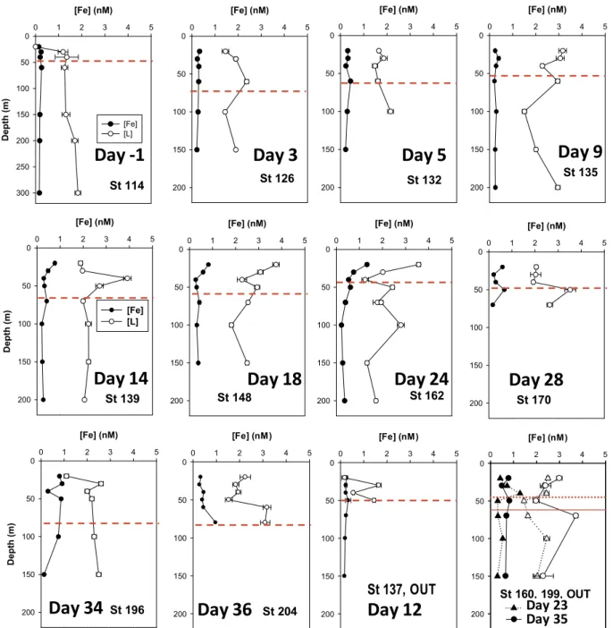
We observed that DFe concentrations in the upper 200 m were barely changed by the two fertilizations (both equivalent to 120 μmol Fe m−2, i.e.: 2.4 nM over the upper 50 m, the pre-fertilization MLD). However, after 14 days, coinciding with the peaking of Chl-a concentrations, DFe profiles became patchily distributed and with increasing concentrations down to 200 m (Figs. 2 and 3A). This distribution is indicative of transfer from the particulate to the dissolved fraction. Copepod fecal pellet counting and analysis of their iron content allowed us to de- termine the contribution of copepod fecal pellets to the standing stocks of particulate iron. We estimated that after the second fertilization, the percentages of DFe, iron in copepod fecal pellets and iron in the rest of particulate material (biological and mineral phases) in fertilized waters in the upper 80 m were approximately constant at 25, 40 and 35%, respectively (equivalent approximately to concentrations of 0.6, 1.1 and 1.0 nM Fe, respectively). Increased and patchy DFe concentration determined during the last two stages of the experiment would be mainly the result of “sloppy feeding” (the process where approximately 50% of food is dispersed as DOC during prey crushing before ingestion) (Møller et al., 2003). Here, we assume that iron binding ligands in- cluded in cells and fecal pellets, are spilled in a similar percentage. The iron content ofC.simillimusfecal pellet was ~5 fold higher if the co- pepod had been captured in fertilized waters (0.041 ± 0.019 vs Fig. 1.Top: Globe map (Google Earth) showing the location of the LOHAFEX
experiment. Middle: Chlorophyll-a concentrations including the fertilized patch (irregular red area inside) from a satellite image obtained 2 weeks after the initial fertilization (27 January 2009, Station 114). The gray lines show the trajectories of the buoys deployed to track the fertilized patch. Dates mark the position of stations in fertilized waters and stations in non fertilized waters are marked with the station code (seeTable 1for further details). Bottom: Tem- poral evolution of Chl-a concentrations in the upper 200 m of the water column of the fertilized patch during the LOHAFEX experiment. The different stages of the experiment (growth, grazing and dilution) are indicated by the colored double arrows. The white dashed line indicates the mixed layer depth (MLD).
The two fertilizations are indicated by the two vertical orange lines. (For in- terpretation of the references to color in this figure legend, the reader is referred to the web version of this article.)
0.006 ± 0.009 nmol Fe pellet−1). Lower Chl-a concentrations in non- fertilized waters were not explained by DFe concentrations (similar to fertilized water) but by the lower iron concentrations found in copepod fecal pellets. Rapid recycling of iron-loaded copepod fecal pellets in the upper 100 m of the water column provided the iron required for the longevity of the LOHAFEX bloom.
2. Materials and methods 2.1. Trace clean sampling
A detailed description of sampling and iron analysis protocols can be found elsewhere (Laglera et al., 2017). Iron speciation samples were collected immediately after collection of partitioning samples from the
same Go-Flo bottles. Briefly, samples from the water column, usually down to 200 m, were collected in Teflon-coated 5 L Go-Flo bottles mounted in an epoxy coated aluminum frame (all from General Ocea- nics). Speciation samples were collected at 16 stations (Table 1): one before fertilization, 13 in fertilized waters during the experiment and 2 in non-fertilized waters. Once on deck, the Go-Flo bottles were moved to the laboratory and fixed to a vertical stand inside an overpressurized particle-free plastic “bubble”. Seawater was filtered through poly- carbonate sterile capsules (0.2 μm, Sartobran 300) after pressurizing the Go-Flo bottle head space with 0.2 μm filtered high purity nitrogen.
Samples for iron speciation were stored in 500 mL LDPE bottles, im- mediately frozen and stored in freezers for months before being thawed overnight the day before analysis.
[Fe] (nM)
0 1 2 3 4 5
0
50
100
150
200
St 160, 199, OUT
[Fe] (nM)
0 1 2 3 4 5
0
50
100
150
200 St 170
[Fe] (nM)
0 1 2 3 4 5
0
50
100
150
200 [Fe] (nM)
0 1 2 3 4 5
0
50
100
150
200 St 204
[Fe] (nM)
0 1 2 3 4 5
0
50
100
150
200 St 162
[Fe] (nM)
0 1 2 3 4 5
0
50
100
150
200 St 148
[Fe] (nM)
0 1 2 3 4 5
Depth (m)
0
50
100
150
200 St 196
[Fe] (nM)
0 1 2 3 4 5
Depth (m)
0
50
100
150
200
[Fe]
[L]
St 139
[Fe] (nM)
0 1 2 3 4 5
0
50
100
150
200
St 135
[Fe] (nM)
0 1 2 3 4 5
0
50
100
150
200 St 132
[Fe] (nM)
0 1 2 3 4 5
0
50
100
150
200
St 126
[Fe] (nM)
0 1 2 3 4 5
Depth (m)
0
50
100
150
200
250
300
[Fe]
[L]
St 114
Day -1 Day 5 Day 9
Day 14 Day 18 Day 24 Day 28
Day 3
St 137, OUT
Day 12 Day 23
Day 35
Day 36 Day 34
Fig. 2.Vertical distribution of DFe and iron binding ligands (1 type of ligand model) measured in the upper water column during the LOHAFEX experiment. The dashed red lines indicate the MLD (details in (Martin et al., 2013). Note the different depth scale at Station 114, day −1. Station 137 (day 12) sampling started in fertilized waters, however, it is probable that the ship drifted from fertilized waters during sample collection. DFe and L concentrations found in two stations sampled in non fertilized waters are shown in the last plot (solid line, MLD at station 199). (For interpretation of the references to color in this figure legend, the reader is referred to the web version of this article.)
2.2. Equipment and reagents
Electrochemical analyses were performed in a 663 VA stand (Metrohm AG) provided with a hanging mercury drop electrode (HMDE), a glassy carbon counter electrode, and an Ag/AgCl reference electrode. Signal collection and peak treatment was executed with a μAutolab voltammeter and the GPES software (Eco Chemie B.V.).
Ultrapure water was purified using an Elix/Milli-Q apparatus (Millipore). Ammonia (UltraTrace, Sigma) was of the maximum com- mercially available purity. Iron standards were dilutions in acidified Milli-Q water (pHNBS= 2.0) of an atomic absorption spectrometry standard solution (BDH). The ligand added to form an electrolabile complex with iron was 2,3-dihydroxynaphthalene (DHN, Merck) that was dissolved in bi-distilled methanol at a concentration of 20 mM. The catalytic/buffering solution required for the method was a combined solution of 0.4 M piperazine-N,N′-bis-(2-hydroxypropanesulfonic) acid (POPSO, Sigma-Aldrich) and 0.1 M potassium bromate (AnalaR, BDH) brought to pHNBS8.1 with ammonia. Trace metal impurities were re- moved after repeating twice the following procedure: addition of a MnO2suspension, swirling during 24 h to promote the adsorption of iron impurities to the colloid, and gravity filtration (0.2 μm) to remove MnO2. The iron contamination from all reagents (DHN + BrO3+ POPSO) (analytical blank) was determined by tripling their individual concentration during the analysis of ultrapure water and was found to be 0.06 nM.
2.3. Dissolved iron
The methodology followed for the analysis of the concentration of dissolved iron has been described in detail in a previous paper (Laglera et al., 2017). Briefly, two different analytical techniques were used:
onboard Adsorptive Cathodic Stripping Voltammetry (AdCSV) as in (Laglera et al., 2013b) in an effort to contribute to the tracking of the patch and lab-based Inductively Coupled Plasma-Mass Spectroscopy (ICP-MS) as in (Tovar-Sánchez, 2012) in stored samples. In a subset of samples kept for analysis by both methods we obtained a robust agreement (see (Laglera et al., 2017) for more details).
2.4. Iron speciation
Iron speciation was determined after iron titration by CLE-AdCSV in the presence of DHN, BrO3−(catalytic reagent) and POPSO (buffer). A detailed description of the analytical protocol can be found elsewhere (Laglera et al., 2011;van den Berg, 2006). Briefly, a 120 mL sample was mixed in a LDPE bottle with DHN (final concentration 0.5 μM DHN, log αFe′-DHN= 2.81) and split into 12 aliquots placed in 30 mL poly- carbonate containers. Nine of the containers were spiked with in- creasing iron concentrations in the range from 0.3 to 18 nM, and all of them were left to equilibrate overnight in a refrigerator (typically for 16 h). The first aliquot was used to condition the electrochemical cell and the result of this analysis was not considered. Two hours before analysis the samples were allowed to reach room temperature in the dark. After addition of a POPSO/borate mixed solution, AdCSV analysis gave the concentration of iron sequestered by DHN (known as labile iron) at increasing DFe concentrations (titration data). The percentages of labile iron with respect to DFe in aliquots not spiked with additional Fe can be found inTable 2.
The treatment of titration data allows the determination of the concentration of natural ligands with the ability to complex iron ([L]) and the conditional stability constant of their complexes (K′Fe′L).The underlying mathematical background of how [L] and K′Fe′Lare obtained can be found elsewhere (Gledhill and van den Berg, 1994) and it has been critically discussed several times (Gerringa et al., 2014; Laglera et al., 2013a; Pižeta et al., 2015). Briefly, the titration data (labile versus total iron concentrations) were plotted and the final straight part of the plot was used to calculate the sensitivity. This sensitivity was not corrected following iterative methods (Turoczy and Sherwood, 1997) or fitted combined with the complexing parameters (Sander et al., 2011) for two reasons: i) maximum iron additions were considerably in excess of the complexing capacity (4 to 20 fold) (Laglera et al., 2013a) pro- ducing data sets with very good linearity in their final section and ii) when we tried the effect of the two referred corrections, solutions clearly spread out due to the introduction of several clear Fig. 3.Time course of the concentration of dissolved iron (A) and iron binding
ligands (B) in the upper 200 m of the water column of the fertilized patch during the LOHAFEX experiment. The red lines indicate the two fertilization events. The different stages of the experiment are indicated with color coded double ended arrows. The mixed layer depth, indicated with white rectangles linked by a dashed yellow line was around 50–60 m in the first 3–4 weeks and deepened to around 80 m thereafter. Red crosses in B indicate those samples where it was possible to resolve two types of ligands (seeTable 3andSection 3.4for detailed information). All concentrations in nM. (For interpretation of the references to color in this figure legend, the reader is referred to the web version of this article.)
Table 1
Summary of LOHAFEX stations where the water column was sampled for the analysis of iron speciation.
Station Days after 1st fertiliz. Days after 2nd fertiliz. Features
114 −1 – Initial conditions
121 2 – IN
126 3 – IN
132 4.9 – IN
135 9 – IN
137 13 – Intended IN
139 14 – IN
148 18 – IN
160 23 2 OUT
162 24 3 IN
170 27 6 IN
196 34 13 IN
199 35 14 OUT
204 36 15 IN
Table 2
Complexing parameters and dissolved labile iron concentrations and the percentage of DFe recovered as Fe-DHN obtained by CLE-AdCSV in the presence of 0.5 μM DHN after overnight equilibration. < LOD: linear iron titration to which no ligand concentration could be determined. sd: standard deviation. sd r with the format
> valueindicate that K′ determined during the fitting of a titration data set was lower than its associated error (ΔK′) which impeded the calculation of log(K′ − ΔK′).
In those cases, we used log(K′ + ΔK′) as an approach to the minimum error associated to the calculation of log(K′).
Station Exp. days Depth (m) [Fe]diss(nM) [L] (nM) sd log K′ sd log αFeL [Fe]lab(nM) % labile
114 −1 20 0.14 < LOD – – – – 0.22 157%
114 −1 30 0.20 1.2 0.2 11.85 0.21 2.80 0.17 56%
114 −1 40 0.26 1.3 0.5 11.69 0.50 2.72 0.17 66%
114 −1 60 0.25 1.3 0.1 11.55 0.21 2.55 0.22 84%
114 −1 100 0.27 2.0 0.2 11.82 0.19 3.24 0.10 36%
114 −1 150 0.32 1.3 0.2 11.25 0.17 2.25 0.27 81%
114 −1 200 0.22 1.7 0.1 11.49 0.19 2.66 0.22 90%
114 −1 300 0.17 1.8 0.1 11.69 0.21 2.88 0.15 50%
121 2 20 0.32 1.9 0.1 11.60 0.14 2.79 0.22 66%
121 2 40 0.30 1.9 0.1 11.56 0.14 2.76 0.20 64%
121 2 60 0.28 1.8 0.2 11.68 0.23 2.86 0.19 64%
121 2 100 0.24 3.9 0.1 11.77 0.08 3.33 0.08 32%
126 3 20 0.33 1.5 0.1 11.65 0.35 2.69 0.24 69%
126 3 30 0.23 1.9 0.1 12.44 0.28 3.66 0.03 13%
126 3 60 0.30 2.4 0.1 12.24 0.65 3.55 0.06 20%
126 3 100 0.29 1.4 0.1 12.27 0.28 3.34 0.05 17%
126 3 150 0.26 1.9 0.1 12.12 0.10 3.35 0.05 24%
132 5 20 0.31 1.7 0.1 12.17 0.22 3.29 0.05 16%
132 5 30 0.32 1.9 0.1 12.05 0.76 3.24 0.07 20%
132 5 40 0.23 1.5 0.1 11.81 0.46 2.91 0.06 26%
132 5 60 0.43 1.6 0.1 11.87 0.29 2.95 0.12 28%
132 5 100 0.29 2.2 0.1 11.91 0.37 3.18 0.04 12%
135 9 20 0.24 3.2 0.2 11.82 0.21 3.28 0.04 16%
135 9 30 0.39 3.1 0.2 11.71 0.14 3.13 0.05 12%
135 9 40 0.28 2.3 0.1 11.81 0.12 3.11 0.12 40%
135 9 60 0.21 2.9 0.1 12.01 0.16 3.45 0.01 7%
135 9 100 0.29 1.5 0.1 11.59 0.18 2.67 0.18 58%
135 9 150 0.24 2.0 0.1 11.63 0.07 2.87 0.11 42%
135 9 200 0.25 3.0 0.1 12.28 0.37 3.71 0.02 7%
137* 13 20 0.25 0.18 0.1 11.27 > 0.46 0.30 0.21 81%s
137* 13 30 0.23 1.6 0.1 11.88 0.44 3.03 0.19 80%
137* 13 40 0.23 0.55 0.1 12.38 > 0.44 2.87 0.08 34%
137* 13 50 0.33 1.5 0.1 12.34 0.80 3.38 0.05 16%
139 14 20 0.77 1.9 0.1 12.13 0.70 3.18 0.18 23%
139 14 30 0.48 2.0 0.1 12.20 0.13 3.37 0.07 14%
139 14 40 0.29 3.9 0.2 11.63 0.10 3.18 0.13 45%
139 14 50 0.32 2.7 0.2 11.34 0.08 2.72 0.19 57%
139 14 70 0.42 2.0 0.1 11.95 0.12 3.14 0.19 41%
139 14 100 0.21 2.2 0.1 11.87 0.30 3.17 0.08 37%
139 14 150 0.23 2.2 0.1 12.11 0.35 3.41 0.03 11%
139 14 200 0.27 2.1 0.1 12.45 0.22 3.70 0.03 13%
148 19 20 0.82 3.7 0.1 11.85 0.13 3.32 0.07 9%
148 19 30 0.59 3.1 0.1 11.75 0.11 3.14 0.03 6%
148 19 40 0.27 2.3 0.2 11.32 0.10 2.62 0.13 46%
148 19 50 0.31 2.9 0.1 12.02 0.26 3.44 0.03 10%
148 19 70 0.44 2.5 0.1 11.94 0.09 3.26 0.07 16%
148 19 100 0.32 1.8 0.1 12.08 0.49 3.26 0.09 26%
148 19 150 0.38 2.5 0.1 12.20 0.27 3.52 0.08 20%
162 25 20 1.33 3.6 0.1 11.80 0.09 3.16 0.24 18%
162 25 30 0.75 2.0 0.1 12.22 0.14 3.33 0.11 14%
162 25 40 0.53 1.6 0.1 11.88 0.43 2.88 0.21 33%
162 25 50 0.61 2.4 0.1 11.97 0.21 3.23 0.09 14%
162 25 70 0.40 1.7 0.1 11.79 0.29 3.01 0.09 22%
162 25 70 0.40 1.9 0.1 12.18 0.53 3.37 0.07 17%
162 25 100 0.22 2.7 0.2 11.59 0.14 2.97 0.08 22%
162 25 150 0.28 1.8 0.1 11.67 0.15 2.84 0.09 32%
162 25 200 0.36 2.0 0.1 11.92 0.10 3.13 0.08 22%
170 28 20 0.59 2.1 0.1 11.92 0.18 3.08 0.14 23%
170 28 30 0.21 2.0 0.2 11.25 0.13 2.51 0.15 70%
170 28 40 0.3 1.9 0.1 11.85 0.12 3.06 0.08 27%
170 28 50 0.67 3.5 0.2 11.72 0.22 3.18 0.18 26%
170 28 70 0.17 2.6 0.1 11.50 0.09 2.89 0.16 88%
196 34 20 0.80 1.1 0.1 12.03 0.83 2.49 0.24 30%
196 34 30 0.91 2.6 0.1 12.16 0.59 3.39 0.18 20%
196 34 40 0.30 2.0 0.1 11.64 0.15 2.87 0.22 72%
196 34 50 0.87 2.2 0.1 12.10 0.27 3.23 0.05 6%
196 34 100 0.75 2.3 0.1 12.27 0.63 3.47 0.11 15%
196 34 150 0.13 2.5 0.1 12.21 0.26 3.58 0.06 42%
204 37 20 0.33 2.2 0.2 11.46 0.19 2.74 0.19 57%
204 37 30 0.28 1.8 0.1 11.67 0.18 2.86 0.17 58%
204 37 40 0.46 1.9 0.1 11.95 0.39 3.12 0.15 32%
(continued on next page)
overestimations of the sensitivity. Those same problems with the cor- rection of sensitivity have been identified in prior work with model and
“real” copper titration data (Laglera et al., 2013a).
Scatchard and van den Berg/Ruzic linearizing plots of data for ti- trations (Ruzic, 1982; Sposito, 1982; van den Berg, 1982) showed straight lines for all samples collected at the initial stages of the ex- periment; these results indicate that only a unique class of ligands could be defined. As the experiment progressed and [L] increased, many sets of titration data showed Scatchard plots that were bent (i.e. they di- verged from a straight line); this is indicative of the emergence of a different class of ligand (L1) with an affinity for iron (K′Fe′L1) sig- nificantly higher than the background initial ligands that we will refer in this case as L2(K′Fe′L2). Given this heterogeneity, calculations were repeated in those samples using a two classes of ligand model (L1/K′Fe′L1
and L2/K′Fe′L2). Although nonlinear fitting (Gerringa et al., 1995) was always possible for those titration plots showing linear trends, non- linear fitting to 4 parameters became impossible for most of the curved (i.e. non-straight) plots and we decided to apply to all those data an iterative linear fitting treatment as described before (Laglera-Baquer et al., 2001; Laglera et al., 2013a). To avoid solutions from mixed methods (that confer data different statistical weights) we present here data for a one ligand class obtained with a linear fitting as described before (Ruzic, 1982;van den Berg, 1982). Complexing parameters for all samples considering one single type of ligand are presented in Table 2 whereasTable 3 shows the parameters obtained by the two types of ligands model for those samples where at least data at three different iron concentrations were clearly indicating the presence of more than one type of ligand.
Standard deviations of the complexing parameters were calculated according to the error propagation theory (Monticelli et al., 2010;
Pižeta et al., 2015). As K′Fe′Lis presented in logarithmic units, calcu- lated errors form an asymmetric interval (Gerringa et al., 1995). Stan- dard deviations in Tables S1 and S2 correspond always to the wider side of the interval. When the error was higher than the parameter value, the result is that only one of the limits of the error interval can be calculated in logarithmic units. In those cases we specified with
“ >value” that we are presenting the side of the error interval that was not missing. This failure to produce error estimations was caused in most cases by the few titration data points that we could assign to calculate L1/log K′FeL1(ranging from 3 to 6) since a minimum of 4 data points per ligand is necessary to obtain statistically sound estimates (Gerringa et al., 2014). Large errors introduce uncertainty in the study of temporal and spatial trends of complexation parameters and of their correlation with other variables. For this reason, we avoided the study of single profiles. However, grouping data in standing stocks (see below) for the study of temporal trends, and the use of our whole L1
database for correlation with other variables (nL1= 38), reduces sub- stantially the uncertainty.
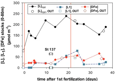
2.5. Integrated iron stocks in the different fractions during LOHAFEX The evolution of ligand concentrations in seawater responds to the combined effect of many biological processes: exudation, degradation, cellular lysis, grazing, microbial activity, etcetera. The complexity provoked by the combination of those effects is reflected in incoherent profiles and spatial patchiness and interferes with the study of temporal trends. We tried to minimize the effect of patchiness by calculating standing stocks of iron and ligands integrating their concentrations over the upper 80 m. The reason behind selecting a fixed depth at 80 m and not the variable MLD was presented before (Laglera et al., 2017).
Briefly, we observed during LOHAFEX that many biological and che- mical parameters showed strong gradients located well below the MLD (white dashed line inFig. 1B) which is routinely calculated with stan- dard criteria based on density gradients. Concentration gradients of Chl-a (Fig. 1A), POC (data not shown) and dissolved (Fig. 2) and par- ticulate Fe (Laglera et al., 2017) were often found below the MLD.
Based on those observations, we selected the maximum depth of Chl-a penetration at 80 m as integration depth (Fig. 4) in order to disentangle the effects of processes carried out by primary producers from those related to grazing and remineralization that can extend further down.
2.6. Study of the analytical restrictions of the dihydroxynaphthalene/
bromate method for the study of iron speciation
Earlier work (Laglera et al., 2011) showed that some CLE-AdCSV protocols (including the DHN/bromate catalytic method used here) could not resolve iron complexation by HS. Briefly, iron complexed with natural ligands must not show any electrolability since natural complexation is calculated by subtracting electrolabile iron from DFe throughout the iron titration (Gerringa et al., 2014). In the presence of bromate, the voltammetric signal of Fe-HS complexes is obtained at the same potential as the Fe-DHN peak (Laglera et al., 2011). Overlapping impedes the isolation of the signal generated by the Fe-DHN complex.
Since the electrolabile fraction is overestimated, the fraction complexed by HS is underestimated to the extent that could go completely un- noticed. As a consequence, the analysis by CLE-AdCSV of UV-digested seawater in the presence of HS and DHN/bromate showed titration plots characteristic of an absence of organic complexation (Laglera et al., 2011). This limitation was verified in our analytical conditions by repeating the analysis of some samples after the addition of 0.12 mg L−1Suwannee River fulvic acid (SRFA, IHSS), equivalent to an increase of the complexing capacity of 2.0 nM (Laglera et al., 2011;
Laglera and van den Berg, 2009;Yang et al., 2017) and 2 nM desfer- roxamine B (DFB, SigmaAldrich) as examples of terrestrial hydrophobic ligands and biologically produced hydrophilic exudates (results given in Fig. S3 and Table S1). Another possible experimental design would have been the addition of those ligands to UV-digested seawater but this Table 2(continued)
Station Exp. days Depth (m) [Fe]diss(nM) [L] (nM) sd log K′ sd log αFeL [Fe]lab(nM) % labile
204 37 50 0.4 1.5 0.1 11.86 0.88 2.91 0.16 39%
204 37 60 0.45 3.2 0.2 11.97 0.27 3.40 0.06 12%
204 37 80 0.97 3.1 0.2 12.48 0.19 3.97 0.07 7%
OUT stations
160 22 20 0.78 3.0 0.1 12.18 0.38 3.53 0.07 9%
160 22 30 0.49 2.4 0.2 11.86 0.67 3.15 0.08 17%
160 22 50 0.82 2.0 0.1 12.04 0.93 3.10 0.09 11%
160 22 70 0.69 3.7 0.1 12.25 0.21 3.73 0.02 2%
160 22 150 0.65 2.3 0.4 11.33 0.32 2.54 0.23 35%
199 35 20 0.43 2.5 0.1 11.63 0.06 2.94 0.17 39%
199 35 30 0.73 2.3 0.0 12.10 0.10 3.30 0.14 19%
199 35 40 1.29 2.4 0.1 12.12 0.55 3.18 0.36 28%
199 35 50 0.32 1.5 0.0 12.17 0.27 3.22 0.06 19%
199 35 70 0.33 1.6 0.1 12.07 0.29 3.19 0.10 28%
199 35 100 0.54 2.4 0.1 12.54 0.17 3.82 0.03 5%
has been previously performed and the results can be found elsewhere (Laglera et al., 2011;van den Berg, 2006). The objectives were: i) de- termine whether the contribution to iron complexation of both model ligands could be determined and ii) if that was the case, to ascribe the added ligand to a specific ligand class (L1or L2).
It should be mentioned that there is another CLE-AdCSV protocol based in the formation of electrolabile complexes of iron with TAC (2- (2-thiazolylazo)-p-cresol) that shows the same analytical limitation to resolve iron complexation by HS (Laglera et al., 2011). This has been confirmed in recent experiments combining iron titrations in the pre- sence of the competing ligands SA (salycilaldoxime) and TAC with HS measurements (data not published). Therefore, since all previous stu- dies about ligand release during OIF experiments (Boye et al., 2005;
Kondo et al., 2008) used TAC as competing ligand, those were also limited to non-humic ligands, facilitating the comparison with the re- sults presented in this work.
In order to ascertain the interference from HS before the start of the experiment, we determined the concentration of HS in three samples (from 20 m deep, days −1 and 13 and 60 m deep from day 0) following an established procedure (Laglera et al., 2007) with internal calibration using the same SRFA standard.
3. Results
3.1. Dissolved iron during LOHAFEX
Even though the temporal evolution of DFe during LOHAFEX was addressed in a previous publication (Laglera et al., 2017), the present study of iron organic speciation requires that we briefly revisit DFe concentrations for those samples where organic complexation was de- termined. Vertical profiles of DFe and ligand concentrations are shown inFig. 2and the temporal evolution of DFe in the fertilized patch down to 200 m inFig. 3A.
Briefly, during thegrowthstage, DFe concentrations down to 200 m were barely increased by the initial fertilization (from ~0.2 to ~0.3 nM despite an addition equivalent to 2.4 nM throughout the ML). This is due to the rapid formation of inorganic colloids wider than our 0.2 μm filters (Laglera et al., 2017). During thegrazingstage (days 14 to 34), DFe concentrations increased moderately down to 200 m but sub- stantially in the upper 40 m of the water column to the range 0.5–0.7 nM with values up to 1.3 nM. This increase was observed before the second fertilization and it was mostly caused by the release of DFe from cells and copepod fecal pellets via sloppy feeding due to the in- crement of the copepod grazing pressure. During thedilutionstage (day 25 onwards), DFe profiles were not affected by the second fertilization and became incoherent with scattered concentrations up to 0.9 nM down to 100 m deep. The same scattering of DFe concentrations was Table 3
Complexing parameters according to a two types of ligands for dissolved samples collected during LOHAFEX. sd: standard deviation. sd with the format > value indicate that K1′ (or K2′) determined during the fitting of a titration data set was lower than its associated error (ΔK1′) which impeded the calculation of log(K1′-ΔK1′).
In those cases, we used log(K1′+ΔK1′) as an approach to the minimum possible uncertainty associated to the calculation of log(K1′). Please note that when the error propagation theory is used on iterative linear fitting, sometimes the statistical uncertainty associated to L1complexing parameters is substantial.
Station Depth (m) [L1] (nM) sd log K1′ sd [L2] (nM) sd log K2′ sd
132 20 0.45 0.55 13.02 > 0.31 1.35 0.14 11.50 0.27
132 30 0.78 0.62 12.44 0.54 1.12 0.26 11.64 > 0.32
132 40 0.57 0.66 12.59 > 0.30 1.16 0.34 11.10 0.43
132 100 0.45 0.65 13.15 > 0.35 1.76 0.20 11.68 0.70
135 20 0.38 0.59 13.14 > 0.36 3.11 0.29 11.41 0.16
135 30 0.42 0.79 13.82 > 0.38 3.28 0.49 11.18 0.17
135 60 0.49 0.91 13.22 > 0.43 2.65 0.20 11.62 0.21
135 200 0.49 1.24 13.39 > 0.52 2.56 0.16 11.93 0.38
139 30 0.56 1.56 12.84 > 0.36 1.50 0.06 11.77 0.17
139 70 0.46 0.97 12.43 > 0.46 1.62 0.08 11.66 0.15
139 150 0.62 1.13 12.94 > 0.42 1.70 0.11 11.84 0.43
139 200 0.47 0.74 12.78 > 0.39 1.62 0.04 12.28 0.40
148 20 0.96 1.52 13.05 > 0.36 3.25 0.36 11.32 0.16
148 30 1.02 1.79 13.89 > 0.40 2.29 0.25 11.31 0.17
148 40 0.38 1.20 12.24 > 0.60 2.67 0.79 10.83 0.22
148 50 0.58 0.91 12.98 > 0.38 2.60 0.22 11.50 0.18
148 70 0.76 0.91 12.74 > 0.31 1.95 0.08 11.48 0.09
162 20 1.57 1.76 12.30 1.28 2.19 0.24 11.40 0.25
162 30 1.27 1.98 12.60 > 0.38 0.76 0.04 11.96 0.60
162 40 0.66 0.93 12.30 > 0.35 0.97 0.41 11.69 > 0.68
162 50 0.49 0.29 13.71 0.25 2.11 0.24 11.55 0.47
162 70 0.87 1.56 12.44 > 0.43 1.11 0.11 11.87 0.71
162 70 0.35 0.45 13.21 1.68 1.46 0.18 11.46 0.32
162 100 0.68 0.85 12.42 > 0.33 2.30 0.38 11.27 0.30
162 150 0.34 0.31 12.66 0.67 1.63 0.29 11.28 0.37
162 200 0.63 0.81 12.39 > 0.33 1.44 0.08 11.65 0.15
170 20 0.58 0.84 12.75 > 0.35 1.59 0.13 11.55 0.23
170 40 0.37 0.12 12.73 0.14 1.67 0.10 11.53 0.15
196 50 1.67 1.35 12.73 0.48 0.75 0.87 10.89 > 0.43
204 60 0.71 0.66 12.95 0.66 2.83 0.40 11.41 0.25
204 80 1.13 2.62 13.50 > 0.46 2.20 0.21 11.89 0.41
OUT stations
160 30 0.94 0.68 12.64 0.43 1.25 0.51 11.33 > 0.36
160 50 0.87 0.76 13.44 0.48 1.21 0.29 11.39 0.98
160 70 0.96 0.37 13.87 0.16 3.10 0.18 11.56 0.12
199 30 0.84 0.79 12.34 0.73 1.51 0.08 11.92 0.33
199 50 0.72 0.41 12.60 0.28 0.83 0.12 11.55 0.41
199 100 1.23 1.36 13.16 > 0.30 1.13 0.38 12.04 > 0.81
199 150 0.33 0.15 12.96 0.19 1.85 0.51 11.25 0.57