Transient Tracers and Eddies along GO-SHIP section A10.5
Bachelor Thesis In Chemistry
Department of Chemistry Christian-Albrecht-University Kiel
Submitted by Lennart Gerke
Kiel, September 2017
Erstgutachter: Prof. Dr. Arne Körtzinger Zweitgutachter: Prof. Dr. Christa Marandino
Kiel, September 2017
The Bachelor thesis was written between July and September 2017 Supervision: Prof. Dr. Arne Körtzinger
Institute of Chemical Oceanography
Christian-Albrecht-University Kiel
iii Table of contents
Abstract……….……….…… v
Zusammenfassung……….……….…… v
1. Introduction……….………. 1
1.1 The cruise……….……….. 1
1.2 Eddies in general……….……….. 1
1.3 The effect of eddies on the ocean circulation……….. 3
1.4 Transient tracers….……….. 3
1.4.1 SF6... 5
1.4.2 CFC´s……….... 6
1.5 The use of transient tracers in the analysis of ocean circulation………. 7
1.6 Transit time distribution…….………. 7
1.7 Mean age….……… 8
1.8 Water masses……….……….. 11
1.9 Aim of the thesis……….……… 12
1.10 The data.………...… 12
2. The Data………...… 13
2.1 Materials and Methods……….………. 13
2.1.1 Determination of CFC and SF6 concentrations……….……... 13
2.1.2 ADCP measurements……….……... 14
2.1.3 Measurement of salinity, oxygen, nutrients, dissolved inorganic carbon (DIC) and total alkalinity (TA)……….…….. 15
2.1.4 Satellite images……….……….… 16
2.1.5 MatLab……….………... 16
3. Results……….……….. 17
3.1 Distribution of different substances along the cruise……….……….… 17
3.1.1 pCFC-12……….……….. 17
3.1.2 pSF6……….………... 18
iv
3.1.3 Salinity……….………. 22
3.1.4 Oxygen……….………. 25
3.1.5 Dissolved Inorganic Carbon (DIC)……….………. 27
3.1.6 Total Alkalinity (TA)……….……… 29
3.1.7 Potential temperature…….……….………... 30
3.2 Acoustic Doppler Currents Profiling along the cruise.……..……….………. 32
4. Discussion……….……… 34
4.1 Eddies………. 34
4.2 Water masses……….……….. 36
4.3 Comparison to historical data……….……….. 37
4.3.1 Comparison of salinity……….. 37
4.3.2 Comparison to oxygen levels……….……….. 38
4.3.3 Comparison of potential temperatures………….……… 38
4.3.4 Comparing SF6 data obtained in from 2017 to CFC-12 data from 2003 39……….………. 38
5. Conclusion……….……….. 40
6. Outlook……….………. 41
Literature……….……….. 42
Appendix……….……… 43
7. Comparing the transient tracers to the other parameters……….……….. 43
7.1 Transient tracers versus salinity……….……….………... 43
7.2 Transient tracers versus temperature……….……….……….. 44
7.3 Transient tracers versus oxygen……….……….……… 45
7.4 Transient tracers versus dissolved inorganic carbon (DIC)…….………….………. 47
7.5 Transient tracers versus total alkalinity (TA)……….……….………… 48
Acknowledgements………. 50
Eidesstattliche Erklärung……….……… 51
v Abstract
This thesis analyzes different ocean parameters that were obtained during a cruise from Cape Town in South Africa to Montevideo in Uruguay in January 2017. A particular emphasis is put on the distribution of the transient tracers CFC-12 and SF6 that can provide information about the movement and circulation of water masses. Moreover, tracer concentrations as well as salinity, temperature and other parameters in different depth along the cruise were used to predict eddies and the influence of these eddies on the parameter distributions and the ocean circulation was examined.
The results show a characteristic upwelling of the different parameters at specific longitudes indicative of two to three eddies along the cruise. The eddies are particularly evident in the ADCP (Acoustic Doppler Currents Profiler) data which also show that one of the eddies is turning clockwise and another one counterclockwise. Detailed analysis of the distribution of the transient tracers and the other parameters also reveals the existence of Antarctic Intermediate Water (AAIW) at a depth from 500 to 1800 m, Antarctic Bottom Water (AABW) close to the bottom and North Atlantic Deep Water (NADW).
Zusammenfassung
In dieser Bachelorarbeit wurden verschiedene Ozeanparameter untersucht, welche während einer Schiffsreise von Kapstadt in Süd Afrika nach Montevideo in Uruguay im Jahr 2017 gemessen wurden. Ein besonderes Augenmerk lag dabei auf der Verteilung der Spurengase CFC-12 und SF6, welche Informationen über die Bewegung und Zirkulation der verschiedenen Wassermassen liefern kann. Außerdem wurden die Verteilung der Spurengase und anderer Parameter, wie Salzgehalt und Temperatur genutzt, um Wasserwirbel, sog. eddies zu bestimmen und den Einfluss dieser auf die Verteilung der verschiedenen Stoffe und die Ozeanzirkulation zu untersuchen.
Die Ergebnisse zeigen an zwei bis drei unterschiedlichen Längengeraden einen Auftrieb der gemessen Parameter, welcher auf eddies hinweist. Diese eddies sind außerdem sehr gut in den ADCP (Acoustic Doppler Currents Profiler) Daten ersichtlich, welche zusätzlich beweisen, dass ein eddy sich im Uhrzeigersinn und ein anderer gegen den Uhrzeigersinn dreht. Eine genauere Betrachtung der einzelnen Parameter und Spurengase beweist darüber hinaus auf die Existenz verschiedener Wassermassen hin, wie dem Antarktischen Zwischenwasser (AAIW) bei einer Tiefe von 500 bis 1800 m, dem Antarktischen Bodenwasser (AABW) nahe dem Grund des Ozeans und dem Nordatlantischen Tiefenwasser (NADW).
1 1. Introduction
1.1 The cruise
In this thesis, the ocean circulations and effects of eddies, large coherent vortices, on the ocean circulation were studied. Moreover, the concentration change of some parameters over the last years was examined. Transient tracers (SF6 and CFC-12) and other parameters were measured and analyzed on a cruise from Cape Town in South Africa to Montevideo in Uruguay in 2017. The cruise was along the latitude of 34.3 °S, according to the SAMOC area (South Atlantic Meridional Overturning Circulation), and was the first cruise crossing the Atlantic Ocean at this latitude. This is of particular interest, because so far measurements at this latitude were only carried out at each coastal region but not in between. The data from another cruise along a latitude of 30 °S from the year 2003 were compared to those of the 2017 cruise thereby revealing potential changes in the distribution of transient tracers and other parameters occurring in the last years.[1] This part of the South Atlantic Ocean has high relevance for the research of eddies, because they frequently form south of South Africa in the Agulhas current.[2]
The cruise was carried out with the vessel named Meria S. Merian between January 4th and February 1st, 2017 and it was led by J. Karstensen. On board, scientist from different countries including Germany, France, Brazil, Argentina, Great Britain and South Africa measured different parameters, such as the transient tracers SF6 and CFC-12, oxygen, temperature, salinity and others.[1]
1.2 Eddies in general
Eddies are coherent vortices in the ocean with a diameter of up to 100 km. They are ubiquitous and half of the kinetic energy of the ocean is contained in all eddies combined. These vortices can turn clockwise and counterclockwise, depending on how and where they emerged. Eddies are characterized by their temperature and salinity anomalies as well as their flow anomalies, with these two anomalies being nearly in geographic equilibrium.[2] They can also be identified in satellite images because the sea level at the center of the eddy is often a few meters lower or higher than the surroundings, which also indicates their vortex motion (clockwise or counterclockwise). Although this appears significant, the difference is rather minute when the size of the eddy is taken into consideration. However, eddies are three-dimensional and the satellite pictures only show the location of the vortices, but they don´t reveal their vertical depth. This information can only be obtained by ADCP (Acoustic Doppler Currents Profiler) measurements or by analyzing transient tracers and other compounds in the eddies and the water masses around the eddies. The direction of the rotation of an eddy also depends on the place they emerge. In the northern hemisphere eddies with a sea level rise in the middle turn clockwise and are called anticyclonic eddies. When they are turning counterclockwise the sea level in the middle is lower and colder. These eddies are then called cyclonic eddies and
2
produce upwelling. On the southern hemisphere this is the opposite way around. On the southern hemisphere, a clockwise turning eddy (cyclonic eddy) causes the sea level to be lower in the middle and a counterclockwise turning eddy produces sea level rise in the center.
The cyclonic eddies with lower sea level in the center are also called cold core eddies and anticyclonic turning eddies warm core.[3] (see figure 1)
Fig. 1: Display of an upwelling and downwelling eddy in the northern hemisphere.[3]
This difference between the northern and the southern hemisphere is caused because of the Coriolis effect. This effect is due to the earths spinning around its axis from west to east.
Because the earth is a sphere points at the equator spin faster than points at the poles.
The majority of the eddies emerge out of currents, like the Golf Stream or the Agulhas Current.
They are formed because of the instability of strong horizontally sheared motions in the boundary of the currents.[2] Eddies can travel along with the current for quite some time before escaping and moving over the ocean on their own. They can also form at regions, where horizontal density gradients are dropping heavily. This is the so called barocline instability.[4]
Eddies can transport warm water and specific properties of nutrients, salt, heat, sediment and other chemicals into different regions of the ocean. For example, vortices account for the majority of oceanic poleward heat transport in the Atlantic across the Antarctic circumpolar current towards the Antarctic.[5] Eddies move nutrients from the deeper interior of the ocean towards the surface and mix the different layers of the Ocean because of their spinning. This can even lead to a plankton bloom at the surface, when many nutrients are carried towards the surface. Moreover, eddies transport nutrients from the ocean towards the coasts, thereby being of crucial importance for the coastal marine life.[2] Eddies transport these different parameters through the ocean, with having them trapped inside of them. The water mass
3
inside the eddy is not able to interact with the water mass of its surrounding. The eddies start emerging and transport the water masses trapped inside of them through the ocean, until they dissolve and the water masses finally interact with the surrounding water masses.
Many eddies found in the South Atlantic that are of majority importance in this thesis originate at the Agulhas current near South Africa. These eddies are very important for transporting warm and salty water northwards towards the North Atlantic. Some of the eddies formed in the South Atlantic will be discussed in more detail.[2]
1.3 The effect of eddies on the ocean circulation
Eddies play an important role in the earth’s climate and have an enormous effect on circulation and transport in the ocean. The ocean in general transports heat and other components from the tropics toward the poles to maintain the tropical climate and distribute heat around the planet. Eddies participate in this process by carrying the heat and other components through the ocean. Another important role of the vortices is the transport of heat towards the ocean surface. Inside an upwelling eddy, water masses are transported from the interior of the ocean to the surface. To some extant this compensates the downward heat flow by the main. Thereby, eddies also take part in regulating the climate and marine ecosystem.[2]
Eddies also have an impact in controlling the ocean characteristics, which change due to climate change. The sea level rises due to climate change. The temperature around the world causes melting ice in the polar regions, which causes a change in the ocean water´s salinity, which in turn results in a change in density. The eddies play a key role in controlling the depth of convection, which occurs because of higher temperatures and melting ice, by mediating the flux of heat from the interior of the ocean into the convection site.[2]
As mentioned above, eddies can be detected in satellite images due to their enormous size or by using ADCP measurements and the analysis of transient tracers like CFC´s or SF6 that will be described below.
1.4 Transient tracers
Transient tracers are usually anthropogenic compounds such as CFC´s and SF6, as well as naturally occurring compounds such as tritium, Argon-39 and Carbon-14. Typically, the appearance of the anthropogenic compounds in the atmosphere is a consequence of human pollution and they enter the ocean via air-sea exchange or water vapor exchange (tritium).
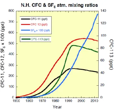
The solubility of the different tracers depends mainly on the temperature of the water and to a smaller extent also on the salinity. At decreasing temperatures, the solubility increases and at increasing salinity, the solubility decreases. The different transient tracers have different atmospheric lifetimes and different atmospheric time histories (see Figure 2). This is due to
4
the production start, for example in 1920 and 1950 (CFC-12 and CFC-11), the productions stop, for example in 1990 (CFC´s) or majorly due to nuclear bomb tests in the 1960s (tritium, Carbon-14).[6]
Fig. 2: Atmospheric time history of the transient tracers CFC´s and SF6 in the Northern Hemisphere.[6]
This atmospheric lifetime is similar all around the world and there is no big difference in the northern and the southern hemisphere in the last 10 years. After the production stop the two hemispheres mixed and the amounts became more similar. Before that the amount of CFC-12 was higher in the northern hemisphere compared to the southern (see Figure 3).
Fig. 3: Atmospheric concentration of CFC-12 between 1980 and 2015 at different points of the hemisphere.[7]
5
Several factors determine which tracer is best suited for the analysis in certain water masses.
These include data on the timescale of the ocean entry/decay of the tracer, the possible involvement and/or consumption of the tracer in biological processes in the water and whether the tracer is easy to measure.[8]
The major transient tracers used for analysis of the ocean circulation and eddies are CFC´s and SF6. These tracers are fairly easy to measure, compared to for example Argon-39, where huge water bottles with lots of capacity must be used to collect sufficient sample. The benefits of measuring SF6 and CFC´s are the smaller bottles for sample collection and that both transient tracers can be measured simultaneously.[9]
1.4.1 SF6
Sulfur hexafluoride (SF6) was first synthesized at the beginning of the 20th century and first produced as an insulating and quenching gas for high voltage systems in the 1950s. It is an inert gas with a low UV degrade rate. The atmospheric lifetime is 3200 years, thus very long.[9]
Sulfur hexafluoride has a chemical structure, in which one sulfur atom is bonded with six fluorine atoms in a square bipyramidal orientation (see Figure 4). This stable structure explains the long lifetime in the atmosphere and low degrade rate. The use of SF6 as a transient tracer is restricted to only very well ventilated water masses. Of course, the partial pressure of the gas in these masses must be above the detection limit of the analytical system.[9] Data from the history of this transient tracer show that SF6 was first detected in late 1900s and the concentration in the atmosphere was calculated back to the late 1950s, when the production and pollution into the atmosphere started. Thereafter, it´s concentration first increased slowly until 1980 and then more rapidly (see Figure 2).
Fig. 4: Schematic display of the square bipyramidal structure of Sulfur hexafluoride (SF6).
SF6 is nowadays used to determine the ocean circulation because an international agreement stopped the use for in situ deliberate release. The vertical eddy diffusion (diapycnal mixing) is now determined with the help of CF3SF5. To measure this, the tracer is added into the water column and then the diffusion over time is measured and analyzed with the help of a gas chromatograph (see Figure 5).[6]
6
Fig. 5: Schematic display of the concentration of a tracer (SF6) in an Eddy over time, also revealing the movement inside the eddy.[6]
1.4.2 CFC´s
There are two major types of Chlorofluorocarbons (CFC´s) used as transient tracers, CFC-12 and the CFC-11. The production of both gases started between 1920 and 1930. They were used as refrigerants, gas propellant, foaming agents and cleaning agents until the production was phased out in 1987 (see Figure 2), due to infrared-mediated detrimental impact. The Montreal Protocol, which declared to stop the use and the production of halogenated hydrocarbons, was signed by 197 nations in 1987. Because the two gases CFC-12 and CFC-11 have an atmospheric lifetime of 90 to 130 years their concentration in the atmosphere only decreases very slowly (see Figure 2). As seen in the historical data from the northern hemisphere, the production of CFC-12 was higher than that of CFC-11 and therefore the concentration of this gas is higher. The CFC-12 concentration increased rapidly from 1950 until the production stop in 1987 before decreasing slowly afterwards. CFC-11 started increasing a little later from 1960 until 1987.[9],[10] This also contributes to its lower concentration in the atmosphere. Because of their atmospheric lifetime, a considerable amount of CFC´s will still be in the atmosphere until the 2100s and probably even longer in the ocean.
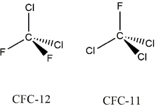
CFC-12 and CFC-11 have a trigonal pyramidal structure consisting of a carbon atom in the middle surrounded by two chlorine atoms and two fluorine atoms in CFC-12 and by three chlorines and one fluorine atom in CFC-11 (see Figure 6). Because there is no source of non-anthropogenic production of CFC´s and because they are not known to be influenced by biological processes, the two gases are ideal candidates of transient tracers. Also, the two compounds exist in most water masses of the oceans. Currently, they are mainly used in analyzing modal ventilation water masses over a timescale of 10 years, such as thermocline ventilation water and the renewal of Antarctic Intermediate Water (AAIW).[10]
7
Fig. 6: Schematic display of the trigonal pyramidal structure of the two CFC´s.
1.5 The use of transient tracers in the analysis of ocean circulation
Transient tracers are used to analyze the ocean circulation and determine eddies. By measuring the concentration of different transient tracers in different water masses at different depth, a mean age of the water masses is determined, i.e. when they had been at the surface to receive gas entry through air-sea exchange. For example, when there are only CFC´s detected in a water mass and no SF6, it must have reached the surface of the ocean between 1920 and 1950 for the last time. The transient tracers are also used to determine changes in ventilation, which changes during the years. With the help of the Transit Time Distribution (TTD) analysis, the ventilation of the ocean can be analyzed.[11] The ocean circulation usually doesn´t change a lot during a short time scale of months, but over years more significant changes can occur that will have an enormous impact on the earth´s climate and the marine ecosystem. This change in the ocean circulation can be compared to the general climate change and it can help determine whether and how one affects the other.
1.6 Transit time distribution
Due to many influencing factors, mixing processes in the ocean are very difficult to quantify.
Because single molecules of a tracer in a water mass cannot be measured, it is important to determine the distribution of a tracer concentration over time. Hall and Plumb (1994) introduced the Transit Time Distribution (TTD) which describes the propagation of tracer boundary conditions into the interior and is based on the Green function (see Equation 1).[12]
𝑐(𝑡𝑠, 𝑟) = ∫ 𝑐0∞ 0(𝑡𝑠− 𝑡)𝑒−𝜆𝑡∙ 𝐺(𝑡, 𝑟)𝑑𝑡 (1) The variable co (ts - t) describes the concentration of the tracer at the source year ts – t related to the input function of the tracer. The exponential function describes the radioactive decay of the tracer with λ being the decay rate (λ = ln(2)/τ1/2 with τ1/2 being the half-life time). The function G (t, r) denotes the Green function and the TTD at the location r. All these factors integrated and multiplicated as shown in equation one yield the tracer concentration (c) in
8
the year (ts) at the location (r), which can be measured. Thus, with a given interior concentration (c (ts, r)) and a given surface time series (ts – t), the Green function can be solved revealing TTD´s for a given tracer.[9]
The TTD can be simplified into the IG-TTD (Inverse Gaussian Transit Time Distribution), when assuming a steady transport of the tracer and steady diffusion gradient and only considering the major compounds of the equation. This generates the following equation (see Equation 2).[9]
𝐺(𝑡) = √ 𝛤3
4𝜋𝛥2𝑡3∙ exp (−𝛤(𝑡−𝛤)2
4𝛥2𝑡 ) (2)
The parameters can be defined as Γ being the mean age, Δ being the width of the distribution and t being the time range. The location r is not considered in this equation, because the sampling point is very distinct. With a given interior concentration equation two can yield limits of the mean age (Γ) and the width of the distribution (Δ) for the distinct location where the sample was taken. The ratio between these two parameters (Γ and Δ) produces information about the advection and diffusion characteristic of the water mass.[9]
For a ratio, larger than 1 (Δ/Γ > 1) the diffusion dominates the mixing and for a ratio below 1 (Δ/Γ < 1), the advection dominates. Ratios higher than 1,8 (Δ/Γ > 1,8) should not be taken into consideration, because higher ratios would lead to a large uncertainty in the mean age. The unity ratio, which is applied to many tracer solutions is Δ/Γ = 1.[9]
For calculating the interior concentration at a certain location, the surface time series of the tracer and equation 1 are used.[12]
All in all, the IG-TTD is very useful for determining the advection and diffusion of the water mass but only for very simplified mixing structures and not for more complex ones.[9]
1.7 Mean age
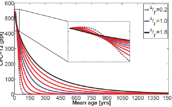
The mean age of a water mass can be deducted from the concentration of the transient tracers measured. With the help of the figures 7 and 8, where the partial pressure of the tracers SF6
and CFC-12 in ppt is plotted against the mean age, the mean age of the water mass can be extrapolated.
9
Fig. 7: Display of the concentration of CFC-12 (in ppt) against the mean age to determine the age of water masses with different Δ/Γ-ratios. Insert shows an enlarged part of the plot at younger mean ages.[9]
Fig. 8: Display of the concentration of SF6 (in ppt) against the mean age to determine the age of water masses with different Δ/Γ-ratios.[9]
Different Δ/Γ-ratios, mean age divided by width of the distribution, are shown from 0.2 to 1.8 with the unity ratio of 1.0 depicted as a solid blue line. As already explained in section 1.6, these ratios were chosen, because ratios higher than 1.8 should be avoided due to large
10
uncertainty in the mean age and ratios below 0.2 also make no sense, because the advection would dominate too much over the diffusion. In the figure of the CFC-12 tracer, the small mean ages are zoomed in, because here very small Δ/Γ-ratios have higher concentrations of the tracer as compared to higher ratios. This is due to the drop of CFC-12 in the atmosphere during the last years because of production stop. However, as this is currently only relevant at very young mean ages, it has no big influence in general yet.[9]
With measuring the concentration of the transient tracers in the water and calculating the distribution and mean concentration, the mean age of the water mass can be calculated. By doing this, the ocean ventilation can be visualized and explained. It can be deducted when a water mass reached the surface for the last time and air-sea exchange took place. Of course, there are ranges between the ratios at certain concentration and the mean age can´t be calculated accurately out of the measured tracer concentration. However, only when the ratios of many tracers show the same results, the mean age can be calculated accurately and with a good approximation.
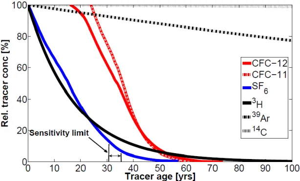
To display the similarity between the two tracers (CFC-12 and SF6) and determine the tracer age in the respective water mass, figure 9 shows the relative tracer concentration plotted against the tracer age.
Fig. 9: Tracer concentration as a function of the corresponding tracer age. For CFC-12 the relative concentration of 100% doesn´t start at a tracer age of 0 years, because the tracer is defined by the atmospheric concentration limit.[9]
The plot displays that the faster the tracer concentration decreases, the shorter is the time when it can be measured. As this is similar at both transient tracers (CFC-12 and SF6), each one of them can be used to determine the age of water masses. The SF6 tracer is younger, which is indicated by the fast decline at very young ages. Therefore, it can be used to calculate the
11
age of younger water masses. The CFC-12 transient tracer is more often used to analyze intermediate- and deep-water masses that are typically older.
1.8 Water masses
The oceans contain several different water masses. Relevant for this thesis are the following:
the Antarctic Intermediate Water (AAIW), the Antarctic Bottom Water (AABW) and the North Atlantic Deep Water (NADW).
The Antarctic Intermediate Water (AAIW) is formed at a high midlatitude of the Southern Pacific Ocean east of the Drake Passage (South of South America) in the junction of the Brazil and Falkland currents.[13] It is formed at latitudes between 50 °S and 60 °S. The water here has very low salinity and is cooled down to about 5 °C. This causes increased density, which is followed by the sinking of the water mass. The AAIW is further formed due to three processes:
first, the midlatitude convection, second the subduction and third the subsurface mixing. All these processes also take place in the Southern and South Pacific Oceans close to the polar region. The subduction is the main process of these three. The water mass is distributing circumpolar in the Southern Ocean and is especially characterized by lower salinity at a depth of around 800 to 1000 m.[14] This water mass spreads far north, even beyond the equator and exchanges with water masses of the northern hemisphere. This all happens at a depth of around 1000 m.[15] This northward spread is observed over the whole longitude of the South Atlantic Ocean.[16]
The Antarctic Bottom Water (AABW), a cold, salty and therefor very dense water, is emerging from the Antarctic. This water mass ventilates the deep ocean and transports oxygen into the interior. Moreover, it plays an important role in the carbon cycle due to the uptake of carbon.
The AABW is formed mainly in the Weddell- and the Ross-Sea. Another region that takes part in the formation of AABW is the counter current of the Antarctic Circumpolar Current (ACC).
Different places reinforce the AABW. They must have a special shape of the coastline, a deep basin or long thin plateau and a polynya system. A polynya system describes an open water mass in between the sea-ice. It can reach a size of more than 85000 km2 and develops because of winds, tides and upwelling warm water masses.[17],[18] All these factors are present at the Mertz Glacier polynya, which is the greatest source region reinforcing AABW. Already a few changes in, for example the shape of the coastline, influence the Antarctic Bottom Water mass and thereby affect the deep-water circulation, the carbon cycle and the climate system. This is due to the high salinity Shelf Water, which is produced because of the changing coastline.[17]
Like the AAIW, the AABW also spreads north over the South Atlantic.
Between the two northward moving water masses (AAIW and AABW) several other water masses flow in from the north, east and west. Among these, the major one is the North Atlantic Deep Water (NADW), which runs southward. The NADW is formed in the Norwegian,
12
Labrador and Greenland Seas during the northern winters, due to cooling of the saline Atlantic surface waters.[19]
1.9 Aim of the thesis
The general aim of this thesis is a better understanding of changes in the ocean ventilation and circulation in the South Atlantic over the last years. By analyzing the distribution of transient tracers and other ocean parameters, a more detailed picture concerning the existence of eddies and their effect on the ocean circulation should be obtained. Data recorded during the cruise in January 2017 should also be compared to data from another cruise that were collected at a similar latitude in the year 2003. The careful analysis of the cruise data should help analyzing the important question whether and to what extent eddies affect the ocean circulation.
In addition to showing the movement of water masses, the transient tracers also give general information about the age of water masses and thereby can help understanding and visualizing the ocean circulation. This information is obtained with the help of the TTD as explained in section 1.6.
1.10 The data
The cruise obtained data on the concentration and distribution of the transient tracers as well as an overview of oxygen content, temperature, salinity, etc. at different locations and depths.
To analyze and evaluate the data, the single concentrations of the substances were plotted against the depth along the cruise section. Furthermore, some substances were also analyzed in two subplots with different limits in the y-axis. Such analysis reveals more detailed information on the first 1000 m in depth and therefore can better link the distribution of these substances to the appearance, movement and extent of eddies.
13 2. The Data
2.1 Materials and Methods
The data on tracer gas concentration and distribution used in this thesis were obtained during a cruise along the GO-SHIP section A10.5. The cruise went from Cape Town in South Africa to Montevideo in Uruguay along the latitude 34.3 °S.[20] During the cruise, different transient tracers, including CFC-12 and SF6, were measured using different methods.
Also considered are earlier measurements along section A10, a little bit north of the cruise from 2017, to reveal differences occurring over the last years. Differences in the concentration/distribution of the tracers, oxygen content and salinity but also in the appearance of eddies were taken into account. Data from this cruise in the year 2003 were obtained from: https://cchdo.ucsd.edu/cruise/49NZ20031106 (22.9.17).
The cruise followed the SAMOC study area (South Atlantic Meridional Overturning Circulation)[20] that displays a very interesting part of the Atlantic Ocean, because it runs parallel to the South Atlantic current. Moreover, as mentioned above eddies emerge from the Agulhas current that flows from the Indian Ocean into the South Atlantic along the South African coast. The ocean section analyzed is located a little north of the Subtropical Front, which separates the Antarctic Circumpolar Current from the South Atlantic gyre.[21]
2.1.1 Determination of CFC-12 and SF6 concentrations
The two tracers were measured efficiently and simultaneously using a gas chromatographic system. This gas chromatograph worked with a purge and trap system and an Electron Capture Detector (ECD), who detected the power drop in the column.[1]
Water samples collected during the cruise were drawn from Niskin bottles and injected into the purge and trap system, followed by the actual gas chromatography that was recorded on a Computer. In more detail, during the purge and trap action, the trap was kept at a temperature between -60 to -68 °C with the help of nitrogen. The sample was then flushed and injected to the purge and trap system. Afterwards the system was heated to a temperature of 110 °C to desorb the trap. The injected gas went from the purge and trap system onto a pre column and then into the main column, where it was measured with the help of the gas chromatograph and detected with the Electron Capture Detector (EDC). All the different columns were kept at a temperature of 50 °C during this whole process. Next to the measured curves of the water samples, standards were measured. Samples containing known, very small amounts of CFC-12 and SF6 gases.[1]
To correct for the non-linearity of the system, calibration curves were measured once a week.[1]
14
Water samples were taken at each measurement station along the cruise. Samples at 22 different depths between the surface and the bottom of the ocean were collected.[1]
2.1.2 ADCP measurements
Acoustic Doppler Currents Profiling was also used to analyze the eddies and the flow velocity of the ocean.
The Acoustic Doppler Currents Profiler (ADCP) is an instrument, which is used to measure the speed and direction of ocean currents. This allows the calculation of the flow velocity at certain points and depths. The principle of the ADCP is based on the Doppler effect.[22]
In brief, the instrument sends out a well-defined acoustic wave at a specific frequency. This wave is then reflected by particles moving in the water. The reflected wave is then also detected by the instrument. The frequency shift between the emitted and reflected wave is used to determine the speed and direction of movement of the particle in the water. This speed and direction is the same as that of the water itself. Particles moving away from the instrument produce reflected waves of lower frequencies returning to the instrument than particles moving towards the ADCP. Because the emitted wave can reach a depth of 1600 m, the circulation and movement of the water can be determined over a considerable distance.
Moreover, water movement in many different depths can be measured at the same time with the ADCP continuously running during the whole cruise. The ships own movement is subtracted from the received flow movement due to a GPS system connected to the ADCP instrument itself. Caution must be taken to keep barnacles and algae from growing on the instrument, which is located at the bottom of the ship.[22]
There are two different types of ADCP´s. One is the ship ADCP (sADCP), which is installed as explained above underneath the ship and measures continuously and the other is the lowered ADCP (lADCP), which is connected to the CTD and lowered into the interior of the ocean at distinct stations. The CTD itself carries different instruments as well as Niskin water bottles or thermometers and is lowered towards the bottom of the ocean via cables. The lADCP thereby provides information on the flow velocity in greater depths, for example below 1600 m, whereas the sADCP, only detects flow velocities up to this depth. However, the lADCP doesn´t measure continuously during the cruise, but only when the CTD is lowered into the interior of the ocean.[1]
Eddies can be detected and analyzed using information on the velocity and direction of water movement obtained by ADCP measurements. Therefor it is important to take into account that ADCP can measure both, the zonal and the meridional velocity. When, for example, the meridional velocity data shows no movement at a specific longitude but there is substantial movement on one side of this longitude in one direction and on the other side in the other direction, an eddy can be predicted at this longitude.[1]
15
The meridional velocity is favored for predicting eddies when the cruise is sailing from east to west or vice versa. The zonal velocity, on the other hand, is used for determining eddies when the ship cruise is going along a longitude from south to north or north to south.
2.1.3 Measurement of salinity, oxygen, nutrients, dissolved inorganic carbon (DIC) and total alkalinity (TA)
The salinity was measured at different depths and locations in the ocean with the help of a salinometer, which was detected to the CTD. Apart from that, the salinity was also measured in water samples taken in the niskin water bottles with two different Salinometers on board.
The OPS (Optimare Precision Salinometer) provided better results than the other did. At each measuring station, 5 to 8 bottles were used to measure salinity at different depth.[1]
The salinometer was calibrated with the help of OSIL standard water samples and home-made substandard water samples.[1]
The oxygen was measured with a technic based on the Winkler´s method. Mangan(II)-chloride, sodium-iodide and sulfuric acid were added and the amount of Iodine is titrated with sodium thiosulphate and measured.[1]
Nutrients were not measured on board but later at the GEOMAR in Kiel. The samples were cooled to a temperature of -20 °C for the transport.[1]
The amount of dissolved inorganic carbon (DIC) was determined by coulometry, followed by SOP#2 (Dickson et al. 2007).[1],[23] At each measurement station samples from all depths were taken and the analysis of dissolved inorganic carbon was carried out.[1]
Total alkalinity (TA), the acid-neutralizing capacity of a water mass, was also measured at all depths of every station. Again water samples were taken and each sample was measured by titration using a potentiometric titration device, followed by SOP#3b (Dickson et al.
2007).[1],[23]
Both parameters, DIC and TA, were determined in one instrument, a coulometer coupled to a Titrino.[1]
16 2.1.4 Satellite images
In addition to the different parameters measured in the water samples, satellite pictures were taken into consideration to analyze the eddy dynamic and structure along the cruise. These show the depth of the water surface and by comparing detailed satellite images eddies can also be predicted. At the center of an eddy the sea level is either a few meters higher or lower than at the boarders, as already explained above. Thus, the exact location of the center of the eddy can be visualized and it is possible to tell whether the cruise passed the center of an eddy or whether the ship sailed closer to one of the boarders of the eddy.
2.1.5 MatLab
The program MatLab[24] was used to display the different parameters measured as functions of one another and plot the different parameters measured along the cruise.
17 3. Results
3.1 Distribution of different substances along the cruise 3.1.1 pCFC-12
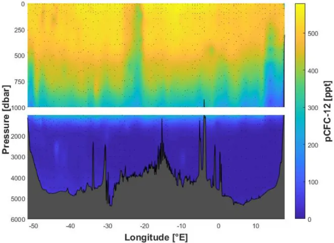
First, I concentrated on the distribution of the transient tracers along the latitude of 34.3 °S at different depths of the ocean. The partial pressure of CFC-12 (pCFC-12) as a function of the cruise section is displayed in the figures 10. The plot is divided at a depth of 1000 m to display the first 1000 m in more detail.
Fig. 10: Schematic display of the partial pressure of the transient tracer CFC-12 (in ppt) along the cruise.
In general, the data show that there is more CFC-12 at the surface of the ocean compared to further depths. From the surface, the amount of CFC-12 is decreasing rapidly during the first 1000 to 1500 m. Below this depth there is no or only very little CFC-12 detected. At a depth of 4000 m, close to the bottom of the ocean, it appears that the concentration of CFC-12 in the water masses starts to increase a little bit again. At the western part of the cruise, the concentrations underneath 2000 m are a little higher than in the eastern part, where there is almost no CFC-12 at these depths.
18
The partial pressure of CFC-12 decreases fast and constantly during the first 1100 m from 550 to 50 ppt and almost reaches its minimum of 0 ppt at 1100 m already. Between 1100 m and almost 1800 m, the decreasing rate is not that high anymore and the minimum of around 0 ppt is reached at 1800 m depth. Moreover, the increase of the tracer at depths below 4000 m is higher in the western part of the cruise at longitudes between 50 °W and 30 °W showing partial pressure of 100 ppt at these depths compared to the increase in the eastern part.
Finally, the plot shows that there are higher amounts of CFC-12 at the surface at longitudes close to the South American Coast (550 ppt) compared to the South African Coast (500 ppt).
Based on the plot in figures 10, eddy structures can be identified at a longitude of 14 °E and 22 °W. At 22 °W the partial pressure of CFC-12 is lower at special depth between 0 to 750 m as compared to the CFC-12 partial pressure at other longitudes at the same depths. The pCFC-12 of 350 ppt is seen at the surface, where normally an amount of 500 to 600 ppt is detected. 350 ppt is detected at a depth of 750 m, when there is no upwelling. The eddy structure at 14 °E is not as strong as the one at 22 °W. There is only upwelling of 350 ppt until a depth of 250 m and not until the surface, but the upwelling partial pressure of CFC-12 is between depths of 250 to 1000 m. At a depth of 1000 m there is a partial pressure of 50 ppt at this longitude. With no upwelling, a partial pressure of 150 ppt would be normal. This can be seen looking in the upper part of the plot, where the first 1000 m are displayed.
At longitudes of 45 °W and 48 °W there are lower partial pressures of 350 ppt seen close to the surface. There is no upwelling at these longitudes, just some water masses showing lower partial pressure at this depth compared to the other longitudes (530 ppt).
3.1.2 pSF6
In the figures 11, the partial pressure of SF6 is shown for different depths along the cruise section. The figure is divided at a depth of 1000 m again to visualize the first part in more detail and to compare the two transient tracer data more easily.
19
Fig. 11: Schematic display of the partial pressure of the transient tracer SF6 (in ppt) along the cruise.
Fig. 12: Schematic display of the partial pressure of the transient tracer CFC-12 (in ppt) in 2003 along 30 °S.
20
The SF6 partial pressure plot shows that the highest amount of SF6 (10 ppt) can be found at the surface and the lowest between 1500 m and 1800 m. The amount of SF6 is decreasing at a very high rate during the first 1000 m and reaches its minimum of 0 ppt at around 1800 m.
In the first 1200 m from the surface there is comparably less SF6 in the eastern part of the cruise at longitudes around 10 °E, than in the western part closer to South America. Amounts of 5 ppt can be detected at a depth of 750 m in the western part as compared to 2 ppt at a longitude of 10 °E. Almost no SF6 is present between 1800 m and the bottom of the ocean, only very miner amounts of 0 to 2 ppt are found at these depths close to the South American Coast. Below 3500 m the amount of SF6 shows this minor increase again, but only in the western part of the cruise at longitudes closer to Uruguay. At the South African coast, there is none SF6 detected at depths below 1800 m.
Again, as in the pCFC-12 data it appears to be a larger difference in the increase of the concentration below 3500 m, where the partial pressure of the tracer is only present in the western part of the cruise.
The upper part of the figure 11 shows at the longitude of 14 °E and 22 °W, the upward shift of lower partial pressure of SF6. At 22 °W the SF6 partial pressure normally found in the water masses taken at a depth of 300 m of 6 ppt are almost present at the surface. At a longitude of 14 °E the range of the upwelling is between depths of 100 and 1000 m. At a depth of 1000 m, the partial pressure of SF6 is at 3 ppt with no upwelling. This specific longitude shows a partial pressure of 0 to 1 ppt at this depth.
At depths between 500 and 1000 m, there is high inconsistency of pSF6 all along the cruise.
The range of the partial pressure at these depths is between 2 ppt and 6 ppt. However, no real upwelling is detected at these depths except for the one at 14 °E.
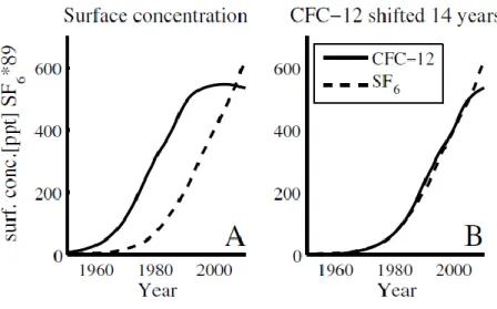
For comparison, data on the partial pressure of CFC-12 obtained along the latitude of 30 °S in the year 2003 are displayed in figure 12. Since the rate of increase of the two tracers CFC-12 and SF6 in the atmosphere is nearly identical but shifted by a time interval of 14 years between them (figure 13), the CFC-12 data from the year 2003 can be compared to the SF6 data from 2017. Thus, at any position in the ocean the measured SF6 partial pressure should be nearly identical to the partial pressure of CFC-12 measured 14 years ago, provided that the flow of the water masses is steady. Differences would therefore indicate that the flow of the water masses changed over the years.[25]
21
Fig. 13: Display of the comparison of the surface concentration of CFC-12 and SF6 with a CFC-12 concentration shifted by 14 years in the right panel.[25]
Figure 12 shows that the partial pressure of CFC-12 is also decreasing from the surface to the bottom of the ocean. However, some differences are apparent when figures 11 and 12 are compared. First, some partial pressure of CFC-12 is detected at almost all longitudes below a depth of 1800 m, whereas no SF6 is found at these levels during the newer cruise. Second, data from 2003 show no upwelling at longitudes of 14 °E or 22 °W, but a downwelling can be seen at a longitude of 2 °W. Here the partial pressure of 350 ppt is detected at a depth of 750, whereas with no downwelling this partial pressure is already measured at a depth of 500 m.
22 3.1.3 Salinity
The data on the salinity along the cruise is displayed in figure 14.
Fig. 14: Schematic display of salinity along the cruise.
Fig. 15: Schematic display of salinity in 2003 along 30 °S.
23
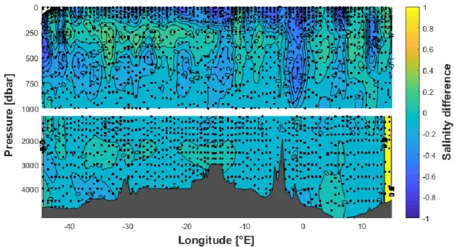
Fig. 16: Schematic display of the relative salinity difference between 2003 and 2017. + indicates more salinity in 2017. – indicates less salinity in 2017.
Figure 14 shows that the highest salinity between 35.6 and 35.7 is at the surface of the ocean.
However, in contrast to what was found for the transient tracers, the salinity shows a clear minimum at around 1000 m depth of 34.2 and then increases again until the bottom. It has to be taken into account that the absolute changes in salinity are not very pronounced as it only varies between 34.2 and 35.7. Closer to the bottom of the ocean, the amount of salinity increases again until 2000 m, where it reaches a value of around 34.8. Salinity then stays relatively constant until a depth of 3200 m, from where it further decreases at a very slow rate until the bottom is reached. This is seen at every longitude.
The figure 14 also shows that surface salinity is higher at longitudes closer to Uruguay (30-50 °W) than in the eastern part of the cruise (0-15 °E). These changes at larger depth and close to the bottom, where the salinity values are slightly higher close to the South African Coast. Thus, it appears that the range of salinity in the South Atlantic is higher in the western as compared to the eastern part.
With the help of the salinity profile shown in figure 14 the eddy structure at the longitude 14 °E can also be identified. Close to the surface, at depths between 0 and 1000 m, a lower salinity can be detected, although the changes are not very pronounced. At a longitude of 22 °W, where the transient tracers clearly showed an eddy structure, the salinity remains rather similar as compared to the other longitudes. There is no upwelling or downwelling visualized.
At 8 °E, 1 °W and 48 °W there is small upwelling visualized in the salinity data. Especially at a longitude of 48 °W the upwelling is more pronounced. Between 100 and 500 m depth, there are always lower amounts of salinity as compared to the other longitudes. This also indicates
24
an eddy, which was not detected in the transient tracer data. At the longitudes 8 °E and 2 °W there are lower amounts of salinity close to the surface between depths from 0 to 200 m. At the surface, the salinity shows 35.2 and not 35.6 to 35.7 as normally at the other longitudes along the cruise.
Close to the South American coast, there are a few measured points at the surface with very low salinity compared to the other longitudes. These points are not considered.
At a depth between 2000 and 3000 m the salinity is a little higher in the western part of the cruise at longitudes between 51 °W and 38 °W. The salinity amount here is at 34.9 as compared to 34.8 at the other longitudes at these depths.
For comparison, data on the salinity in the ocean at a latitude of 30 °S during the year 2003 are shown in figure 15. Data were only collected until a longitude of 45 °W but show the same general decrease in salinity from the surface to the bottom. To a large extent the results from the older cruise (figure 15) are similar to the salinity data from the newer cruise (figure 14).
This also shows the comparison plot (see Figure 16), which displays the exact differences at every depth along the cruise. The only significant differences appear at the surface and at the longitudes where eddies are predicted. At the surface, the salinity is higher in the older data at longitudes close to the South African coast. Where the data from 2017 showed 35.4 salinity, the older data revealed up to 35.7. This 0.3 differential is displayed very well in figure 16. At 14 °E and 48 °W, the older data show no upwelling in the first 1000 m. Only at a longitude of 2 °W some downwelling can be detected at depths between 250 and 1000 m. At this longitude, higher salinity is measured as compared to other longitudes at the same depth. For example, a salinity of 34.9 is detected at a depth of 600 m at this longitude, whereas this salinity is usually reached at a depth of 400 m.
25 3.1.4 Oxygen
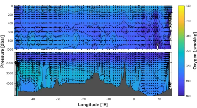
Figure 17 displays the water oxygen levels plotted along the cruise section at the different longitudes and depths. The upper figure gives a more detailed look on the first 1000 m from the surface as the plot is divided at this depth.
Fig. 17: Schematic display of the amount of oxygen levels (µmol/kg) along the cruise.
Fig. 18: Schematic display of the amount of oxygen levels (µmol/kg) in 2003 along 30 °S.
26
Fig. 19: Schematic display of the difference in the oxygen level between 2003 and 2017. + indicates higher oxygen level in 2017. – indicates lower oxygen level in 2017.
The amount of oxygen has a range of around 160 to 255 µmol/kg in the newer data (see Figure 17). Oxygen first decreases a little bit until around 400 m depth, before increasing again until 800 m depth, where it reaches almost the same amount as at the surface of 250 µmol/kg.
With increasing depth, oxygen then decreases rapidly from 250 to 190 µmol/kg and reaches its minimum at a depth of around 1000 to 2000 m. From here, the amount of oxygen increases again until a depth of 3500 m, before decreasing at a slow rate for the next 500 m and staying constant at 220 µmol/kg from 4000 m depth until the bottom of the ocean.
Comparing the different longitudes, where the oxygen was measured, the range is again larger at the western part of the cruise as compared to the eastern. The amount is always lower close to South Africa and the range of change is not as significant as close to the Uruguay coast.
It should be noted here that only measurements until a longitude of 47 °W were taken and that oxygen levels were not measured all the way to the South American Coast.
Figure 17 clearly shows an oxygen minimum zone at a depth of 1000 to 1800 m. In addition, there are lower amounts of oxygen detected at a depth of around 500 m, but this is only minor compared to the lower concentrations between 1000 and 1800 m. A lower amount of oxygen with 210 µmol/kg is detected at a longitude of 14 °E at a depth of 200 m. At all other longitudes, there is 240 µmol/kg oxygen at this depth.
The oxygen profile also provides clear evidence for eddy structure at the longitude of 14 °E.
Especially in the upper plot, where the ocean depth scale is expanded, the upwelling of water masses with lower oxygen can be detected between depths of 600 to 1800 m. Oxygen values of 190 µmol/kg, which are normally found at depths of around 1800 m, are detected at a
27
depth of 800 m at this longitude. At a longitude of 22 °W, there is no upwelling or downwelling identified. There is also no upwelling detected at a longitude of 48 °W, which is due to the measurement stop at a longitude of 47 °W.
Comparing the amount of oxygen in figure 17 to the amount of oxygen in the ocean at almost the same latitude during the year 2003 (see Figure 18) reveals some differences at depths between 600 and 1000 m. The newer data show higher amounts of up to 250 µmol/kg as compared to the data from 2003, where only up to 220 µmol/kg are detected at these depths.
Moreover, it can be observed that the amount of oxygen is generally 10 to 40 µmol/kg higher in the year 2017 as compared to 2003. This difference is directly displayed in figure 19, which shows the exact difference in oxygen level at every depth and longitude. Higher oxygen levels along the cruise in 2017 are clearly seen at depths between 700 and 1000 m. The upwelling of the oxygen levels at 14 °E seen in 2017 is not detected in the older data; however, these show as upwelling at a longitude of 10°E, with lower oxygen levels observed at depths between 200 and 1000 m as compared to the other longitudes. Lower oxygen levels in the year 2017 are measured at a depth of around 2000 m. This is detected in the differential plot (see figure 19), where the oxygen is about 5 µmol/kg lower in the year 2017 as compared to 2003.
3.1.5 Dissolved Inorganic Carbon (DIC)
The measured data of dissolved inorganic carbon along the cruise section is plotted in figure 20. As with the oxygen measurements, some data towards the western end of the cruise are missing and only measurements until a longitude of 41 °W are shown (see Figure 20).
Fig. 20: Schematic display of the amount of dissolved inorganic carbon (DIC) (in µmol/kg) along the cruise.
28
The amount of dissolved inorganic carbon is the lowest at the surface of the ocean at all longitudes across the South Atlantic with 2090 µmol/kg and the highest at the ground with 2250 µmol/kg. The DIC has a range of 2090 to 2250 µmol/kg. From the surface, DIC increases during the first 1500 m. Thereafter, it decreases at a lower rate until a depth of around 3000 m is reached. Closer to the bottom of the ocean DIC increases again and then reaches its maximum of 2250 µmol/kg.
Comparing the different longitudes there is no significant difference. The amount of dissolved inorganic carbon is rather similar at all longitudinal data points. The only difference is at a depth of 2000 to 3500 m, where there is less DIC in the western part of the cruise (between 20 °W and 40 °W) with 2200 µmol/kg compared to the eastern with 2230 µmol/kg, so there is a higher range underneath 1800 m in the western compared to the eastern part.
Looking at the longitudes, where eddy structures were found in the data of the transient tracers, salinity and oxygen, there is an indication of some structure at the longitude of 14 °E again. Upwelling of lower water masses containing higher levels of dissolved inorganic carbon can be recognized very well at depths between 100 and 1000 m. At these depths, there are always higher amounts of DIC as compared to the other longitudes at this depth. At a depth of 600 m, for example the amount of DIC at this longitude is 2180 µmol/kg. At all other longitudes along the cruise the amount is at 2160 µmol/kg at this depth. At the longitude of 22 °W, where there is evidence for an eddy structure seen in the transient tracer data, no significant change in the DIC values compared to other longitudes is observed.
Interesting is the lower DIC amount of under 2100 µmol/kg at a depth of 350 m at a longitude of 34 °W. At all other longitudes at this depth, the amount of DIC always has a value of 2120 µmol/kg. This lower DIC is not due to an upwelling or downwelling process.
29 3.1.6 Total Alkalinity (TA)
Figure 21 shows the Total Alkalinity plotted along the cruise. As for oxygen and DIC, data were not collected along the whole cruise, only up to a longitude of 41 °W. As in all the other plots, the TA is divided at a depth of 1000 m to display the upper part in more detail.
Fig. 21: Schematic display of the amount of total alkalinity (TA) (in µmol/kg) along the cruise.
The inspection of figure 21 reveals that the highest TA, so the highest concentration of alkaline substances in a water mass, is found at the bottom of the ocean and that TA is lowest at a depth of 600 to 900 m. In total, the TA levels range from 2280 to 2370 µmol/kg.
At the surface, TA shows an amount of around 2330 to 2350 µmol/kg, with higher values in the western part of the cruise compared to the South African coast. Then, it decreases in the first 800 m until it reaches its minimum of 2280 µmol/kg. From here, it increases at a high rate until a depth of around 1500 m. It then stays constant for another 1000 m before increasing again until the bottom, where the amount of total alkalinity reaches its maximum of 2370 µmol/kg.
Comparing the different longitudes, reveals no real difference, except for the higher amount of TA at the surface close to the South American coast compared to the South African coast.
The upper panel, shows an eddy structure at a longitude of 14 °E, where an up-flow of water masses with lower TA can be identified at depths between 200 and 1000 m. For example at a depth of 600 m the amount of TA at this longitude shows 2300 µmol/kg compared to the other longitudes along the cruise, where at this depth 2290 µmol/kg is normal. At a longitude of 22 °W, there is again no upwelling or downwelling detected and so there is no eddy structure visualized in the total alkalinity data here. Rather at some other longitude at 8 °E, an upwelling is detected. The lower amount of TA from a depth of 300 m reaches up until the surface. At
30
this longitude the TA at the surface displays 2320 µmol/kg. Normally at the surface, the total alkalinity reveals values between 2340 and 2350 µmol/kg.
3.1.7 Potential temperature
Figure 22 shows the section profile of the potential temperature at the different longitudes.
The potential temperature is a dimension that helps compare different temperatures at different depths. It considers the different pressures at each depth.
Fig. 22: Schematic display of the potential temperature (in °C) along the cruise.
Fig. 23: Schematic display of the potential temperature (in °C) in 2003 along 30 °S.
31
Fig. 24: Schematic display of the potential temperature difference between 2003 and 2017. + indicates higher temperature in 2017. – indicates lower temperature in 2017.
The plot of the newer data shows that during the first 500 m from the surface the temperature decreases rapidly from around 24 °C to 4 °C. At 4 °C the temperature stays constant between depths of 750 m to 3000 m, before decreasing again to around 1 °C and then staying constant until the bottom is reached. There is no real difference between the measurements at the different longitudes, only at depths below 4000 m some variations are seen with water temperatures at the South American coast being slightly lower than those closer to the South Africa coast. Temperatures of 0 °C are measured at longitudes between 50 °W and 35 °W, as compared to 1 °C in the eastern part of the cruise
At a longitude of 14 °E there is a lower temperature at depths of between 250 m to 700 m compared to all the other longitudes. This upwelling of colder water masses is again indicative of eddy structure. Also at a longitude of 48 °W, there is very little up-flow displayed in the data. This could possibly also indicate an eddy. The upwelling at a longitude of 48 °W reaches from depths of 100 to 750 m.
The profile of the potential temperature of the year 2017 can also be compared to the data from the year 2003 (see figure 23). In 2003, the temperature also decreases fast during the first 1000 m before staying constant at 3 °C until a depth of 3500 m and then decreasing further below that depth. Differences between the temperature profiles in 2003 and 2017 are mainly seen at depths close to the surface of the ocean (see Figure 24). The temperature difference at the surface is about 1 °C, displayed clearly in the differential plot in figure 24.
Higher temperatures are found at depths between 100 and 200 m in the year 2003 as compared to 2017. This indicates that the rate of temperature decrease with depth was slightly less rapid in 2003. As observed above for the other parameters, figure 23 also shows
32
no upwelling at longitudes of 14 °E and 48 °W, but shows downwelling at 2 °W between 250 and 1000 m.
3.2 Acoustic Doppler Currents Profiling along the cruise
ADCP measurements were performed to assess particle movements in the ocean waters up to a depth of 1600 m. These are shown in figures 25 for the meridional velocity along the latitude of 34.3 °S.
Fig 25: Display of the meridional velocity along the cruise.[1]
As explained in section 2.1.2, these meridional velocity data can be used to determine the existence of eddies along the cruise from Capetown to Montevideo. Figure 25 reveals that there is no north or south direction in the flow at a longitude of 14 °E and 48 °W. At each side of these longitudes the flow runs in different directions. This clearly indicates the existence of eddies. At a longitude of 22 °W, where the CFC-12 and SF6 data predicted an eddy, no eddy is detected in the ADCP data.
The two eddies at longitudes of 14 °E and 48 °W show opposite flow directions. At 14 °E the water is first moving southward and, after the center of the eddy, turning northward, with respect to the westward moving cruise. This indicates a clockwise turning eddy at 14 °E. At 48 °W this is the opposite way around, showing that this is an eddy turns counterclockwise.
The zonal velocity (see figure 26), which is normally used to determine eddies on a cruise from north to south or south to north shows different flows at longitudes of 14°E, 22 °W and 48 °W.
33 Fig. 26: Display of the zonal velocity along the cruise.[1]
It shows one flow direction at a longitude of 48 °W and flow in two directions at a longitude of 14 °E and 22 °W.
![Fig. 1: Display of an upwelling and downwelling eddy in the northern hemisphere. [3]](https://thumb-eu.123doks.com/thumbv2/1library_info/5330521.1680688/7.892.106.714.262.639/fig-display-upwelling-downwelling-eddy-northern-hemisphere.webp)