Universit¨ at Wuppertal, WS 2017
J¨ urgen M¨ uller
0 Reminder: Determinants 1
(0.1) Signs. . . 1
(0.2) Determinants. . . 1
(0.3) Theorem: Multiplicativity. . . 1
(0.4) Theorem: Laplace expansion. . . 2
(0.5) Example: Direct current networks. . . 2
(0.6) Motivating example. . . 5
1 Rings and polynomials 5 (1.1) Monoids. . . 5
(1.2) Rings. . . 5
(1.3) Factorial domains. . . 6
(1.4) Euclidean domains. . . 7
(1.5) Theorem: Euclid implies Gauß. . . 8
(1.6) Polynomial rings. . . 9
(1.7) Theorem: Polynomial division. . . 10
(1.8) Corollary: Polynomial implies Euclid. . . 10
(1.9) Evaluation. . . 11
2 Eigenvalues 11 (2.1) Similarity. . . 11
(2.2) Eigenvalues. . . 12
(2.3) Eigenvalues of matrices. . . 13
(2.4) Characteristic polynomials. . . 14
(2.5) Diagonalisability. . . 15
(2.6) Example: Fibonacci numbers. . . 16
3 Jordan normal form 17 (3.1) Generalised eigenspaces. . . 17
(3.2) Minimum polynomials. . . 18
(3.3) Theorem: Cayley-Hamilton. . . 19
(3.4) Principal invariant subspaces. . . 19
(3.5) Diagonalisability again. . . 20
(3.6) Jordan normal form. . . 21
(3.7) Triangularisability. . . 23
(3.8) Example: Damped harmonic oscillator. . . 24
4 Bilinear forms 27 (4.1) Adjoint matrices. . . 27
(4.2) Sesquilinear forms. . . 28
(4.3) Gram matrices. . . 29
(4.4) Orthogonal spaces. . . 30
(4.5) Orthogonalisation. . . 32
(4.6) Signature. . . 33
5 Adjoint maps 38
(5.1) Adjoint maps. . . 38
(5.2) Normal maps. . . 39
(5.3) Unitary maps. . . 40
(5.4) Theorem: Spectral theorem. . . 40
(5.5) Corollary: Unitary and hermitian maps. . . 41
(5.6) Principal axes transformation. . . 41
0 Reminder: Determinants
(0.1) Signs. Forn∈N0 letSn be the symmetric group on the set{1, . . . , n}, and thesignmap sgn : Sn→ {±1}:π7→Q
1≤i<j≤n
π(j)−π(i)
j−i = (−1)l(π), where l(π) :=|{{i, j};i < j, π(i)> π(j)}| ∈N0 is itsinversion number. Ifρ∈ Sn
is a k-cycle, for some k ∈ N, then we have sgn(π) = (−1)k−1; in particular sgn(id) = 1, and for atransposition σ∈ Sn we have sgn(σ) =−1.
Forπ, ρ∈ Snwe havemultiplicativitysgn(πρ) = sgn(π)·sgn(ρ), and we have sgn(π−1) = sgn(π). The elements ofAn:={π∈ Sn; sgn(π) = 1}andSn\ An = {π ∈ Sn; sgn(π) = −1} are called even and odd permutations, respectively;
thenAn≤ Sn is a subgroup, being called the associatedalternating group.
(0.2) Determinants. a) Let K be a field. Then the determinant of a square matrix A := [aij]ij ∈ Kn×n, where n ∈ N0, is defined as det(A) :=
P
π∈Snsgn(π)·Qn
j=1aπ(j),j ∈K.
For example, for anupper triangular matrixA ∈Kn×n, that is aij = 0 for all i > j ∈ {1, . . . , n}, we get det(A) = Qn
j=1ajj ∈ K; in particular, for the identity matrixEn∈Kn×n we get det(En) = 1.
Forn= 0 we have det([]) = 1; forn= 1 we have det([a]) =a; forn= 2 we have det
a11 a12
a21 a22
= a11a22−a12a21; for n = 3 we have det
a11 a12 a13
a21 a22 a23
a31 a32 a33
= (a11a22a33+a12a23a31+a13a21a32)−(a13a22a31+a12a21a33+a11a23a32), called theSarrus rule.
b) The map det : (Kn×1)n → K: [v1, . . . , vn] 7→ det([v1, . . . , vn]), where by [v1, . . . , vn] ∈ Kn×n we denote the matrix having columns v1, . . . , vn, has the following properties: It isK-multilinear, that isK-linear in each argument, and it isalternating, that is det(. . . , v, . . . , v, . . .) = 0 for allv∈Kn×1. Hence we have det(. . . , v, . . . , w, . . .) = −det(. . . , w, . . . , v . . .) for all v, w ∈ Kn×1, and det(. . . , v, . . . , w, . . .) = det(. . . , v+aw, . . . , w . . .) for all a∈K.
Moreover, we have det(Atr) = det(A). Hence det is row multilinear and row alternating as well, and the above properties also hold row-wise. Hence this allows to compute the determinant ofAby applying the Gauß algorithm, keep- ing track of the row operations made, and to read off the determinant of its Gaussian normal form which is an upper triangular matrix.
(0.3) Theorem: Multiplicativity. a)ForA, B∈Kn×n we have det(AB) = det(A)·det(B). Hence ifA∈GLn(K) then we have det(A−1) = det(A)−16= 0.
Hence SLn(K) :={A∈GLn(K); det(A) = 1} ≤GLn(K) is a subgroup, being called thespecial linear groupof degreenoverK.
b)IfV is a finitely generatedK-vector space, andB⊆V aK-basis, then the determinantof ϕ∈EndK(V) is defined as det(ϕ) := det(MBB(ϕ)), which by
base changeindeed is independent of theK-basis chosen.
(0.4) Theorem: Laplace expansion. LetA= [aij]ij ∈Kn×n wheren∈N, and fori, j∈ {1, . . . , n}let
Aij:=
a11 . . . a1,j−1 a1,j+1 . . . a1n
... ... ... ...
ai−1,1 . . . ai−1,j−1 ai−1,j+1 . . . ai−1,n ai+1,1 . . . ai+1,j−1 ai+1,j+1 . . . ai+1,n
... ... ... ...
an1 . . . an,j−1 an,j+1 . . . ann
∈K(n−1)×(n−1)
be the matrix obtained fromAby deleting rowiand columnj, where det(Aij)∈ Kis called the (i, j)-th (n−1)-minorofA.
a) Then we havecolumn expansion det(A) = Pn
i=1(−1)i+j·aij ·det(Aij), for allj ∈ {1, . . . , n}, as well asrow expansion det(A) =Pn
j=1(−1)i+j·aij· det(Aij), for alli∈ {1, . . . , n}.
b) Let adj(A) := [(−1)i+j·det(Aji)]ij ∈Kn×n be the adjoint matrix of A.
Then we haveA·adj(A) = adj(A)·A= det(A)·En∈Kn×n.
Hence we haveA∈GLn(K) if and only if det(A)6= 0, and in this case we have A−1= det(A)−1·adj(A)∈GLn(K);
c) For A ∈GLn(K) and w ∈ Kn×1, the unique solution v = [x1, . . . , xn]tr ∈ Kn×1 of the system of linear equationsAv =wis byCramer’s rule given as xi:= det(A)−1·det(Ai(w))∈K, for alli∈ {1, . . . , n}, whereAi(w)∈Kn×n is the matrix obtained fromAby replacing columnibyw.
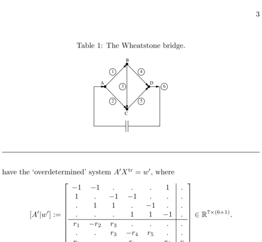
(0.5) Example: Direct current networks. We consider the Wheatstone bridge as depicted in Table 1: We have electrical connections between the vertices (A, B), (A, C), (B, C), (B, D), (C, D), and (D, A), whose internal resistances are given as r := [r1, . . . , r6] ∈ R6, respectively, where rj > 0.
Voltage v ∈ R is fed into (D, A), and the task is to determine the currents c:= [c1, . . . , c6]tr∈R6×1 in the connections. In particular, we wonder whether it is possible to adjust the internal resistances such that the currentc3 through the bridge (B, C) vanishes.
By Kirchhoff ’s laws, incoming and outgoing currents cancel out at each of the vertices A, B, C, D, leading to the first four of the following equations.
Moreover the voltage between two vertices is given as the product of the internal resistance and the current, and the voltages cancel out along all closed circuits in the network without source or sink; using the circuits (A, B, C) and (B, C, D) this leads to the next two of the following equations, while using the circuit (A, B, D) the last one is due to the voltagev fed into the network. Hence we
Table 1: The Wheatstone bridge.
1 4
6
5 2
3 A
B
C
D
have the ‘overdetermined’ systemA0Xtr=w0, where
[A0|w0] :=
−1 −1 . . . 1 .
1 . −1 −1 . . .
. 1 1 . −1 . .
. . . 1 1 −1 .
r1 −r2 r3 . . . . . . r3 −r4 r5 . . r1 . . r4 . r6 v
∈R7×(6+1).
Since the currents are accounted for with opposite signs at their respective end vertices, the column sums of the equations coming from the balance of currents all vanish. Thus summing up the first four rows ofA0 yields a zero row, and we may leave out row 4 and look at the systemAXtr =w, where
[A|w] :=
−1 −1 . . . 1 .
1 . −1 −1 . . .
. 1 1 . −1 . .
r1 −r2 r3 . . . . . . r3 −r4 r5 . . r1 . . r4 . r6 v
∈R6×(6+1).
If Kirchhoff’s laws describe direct current networks completely, the above system should have a unique solution. Thus we check thatA∈R6×6 is invertible:
Adding column 6 to columns 1 and 2, and using row expansion with respect to row 1 we get
det(A) =−det
1 . −1 −1 .
. 1 1 . −1
r1 −r2 r3 . . . . r3 −r4 r5
r1+r6 r6 . r4 .
.
Adding ther5-fold of row 2 to row 4, and using column expansion with respect to column 5; and adding column 1 to columns 3 and 4, and using row expansion with respect to row 1, the right hand side equals
−det
1 . −1 −1
r1 −r2 r3 . . r5 r3+r5 −r4 r1+r6 r6 . r4
=−det
−r2 r1+r3 r1 r5 r3+r5 −r4
r6 r1+r6 r1+r4+r6
.
The Sarrus rule implies det(A) = r2(r3+r5)(r1+r4+r6) + (r1+r3)r4r6− r1r5(r1+r6) +r1(r3+r5)r6+ (r1+r3)r5(r1+r4+r6) +r2r4(r1+r6) =r1r2r3+ r1r2r4+r1r2r5+r1r3r5+r1r3r6+r1r4r5+r1r4r6+r1r5r6+r2r3r4+r2r3r6+ r2r4r5+r2r4r6+r2r5r6+r3r4r5+r3r4r6+r3r5r6>0, where the only summand with negative sign cancels out.
Hence we haveA ∈GL6(R), and the system AXtr =w has a unique solution c= [c1, . . . , c6]tr∈R6×1. By Cramer’s rule we have
c3·det(A) = det
−1 −1 . . . 1
1 . . −1 . .
. 1 . . −1 .
r1 −r2 . . . . . . . −r4 r5 . r1 . v r4 . r6
.
Using column expansion with respect to column 3, and column expansion with respect to column 5, the right hand side equals
−v·det
−1 −1 . . 1
1 . −1 . .
. 1 . −1 .
r1 −r2 . . . . . −r4 r5 .
=−v·det
1 . −1 .
. 1 . −1
r1 −r2 . . . . −r4 r5
.
Adding column 1 to column 3, adding column 2 to column 4, and using row expansion with respect to rows 1 and 2, this in turn equals
−v·det
1 . . .
. 1 . .
r1 −r2 r1 −r2
. . −r4 r5
=−v·det
r1 −r2
−r4 r5
.
Hence we have c3·det(A) = v·(r2r4−r1r5). Thus for v 6= 0 the current c3
vanishes if and only if the internal resistances fufillr2r4=r1r5, in other words if and only if we have rr1
2 = rr4
5. ]
The physical interpretation is as follows: The voltage v applied to vertex A is distributed to verticesB and C according to the quotient rr1
2, similarly the voltage−vapplied to vertexD is distributed to verticesB andC according to the quotient rr4
5. There is no current through through the bridge (B, C) if and only ifB andC are on the same potential, thus if and only if rr1
2 = rr4
5.
(0.6) Motivating example. We conclude with a motivating example, indi- cating the aim of the considerations to come next:
We consider V := R2×1 with standard R-basis B, and R-basis C given by MBC(id) =
1 −1
1 1
∈GL2(R); henceMCB(id) = (MBC(id))−1=12·
1 1
−1 1
. i)For thereflectionσ∈EndR(V) at the hyperplane perpendicular to [−1,1]tr we getMBB(σ) =
. 1 1 .
∈R2×2, and MCC(σ) = MCB(id)·MBB(σ)·MBC(id) = 1 .
. −1
∈ R2×2. TheR-basis C seems to be better adjusted to σ, inasmuch MCC(σ) is a diagonal matrix, in other words any vector inC is mapped byσto a multiple of itself.
ii)To the contrary, for therotationρ∈EndR(V) with respect to the angleω∈ Rwe getMBB(ρ) =
cos(ω) −sin(ω) sin(ω) cos(ω)
∈R2×2. Forω 6∈πZit is geometrically clear that there is no non-zero vector being mapped byρto a multiple of itself.
Hence the question arises, under which circumstances such nicely adjusted bases exist, and if so how to find them.
1 Rings and polynomials
(1.1) Monoids. A setM together with amultiplication·:M×M →M ful- filling the following conditions is called amonoid: There is aneutral element 1 ∈ M such that 1·a =a =a·1 for all a∈ M, and we have associativity (ab)c=a(bc) for alla, b, c∈M. If additionallyab=ba holds for alla, b∈M, thenM is calledcommutativeorabelian.
An elementa∈M is calledinvertibleor aunit, if there is aninversea−1∈M such thataa−1= 1 =a−1a. In this case, if a0 ∈M also is an inverse, we have a0= 1·a0=a−1aa0=a−1·1 =a−1, hence the inverse is uniquely determined.
LetM∗ ⊆M be the set of units. Then we have 1∈M∗, where 1−1 = 1; for alla, b∈M∗ we fromab(b−1a−1) = 1 = (b−1a−1)abconclude ab∈M∗, where (ab)−1=b−1a−1; and we have (a−1)−1=a, thusa−1∈M∗.
A monoid M such that M∗ = M is called a group. In particular, for any monoidM the subsetM∗is a group, called the group of unitsofM.
For example, N0 is a commutative additive monoid with neutral element 0, and N is a commutative multiplicative monoid with neutral element 1, while Zis a commutative additive group with neutral element 0, and a commutative multiplicative monoid with neutral element 1.
(1.2) Rings. a)A setRtogether with an addition + : R×R→R and a mul- tiplication·:R×R→Rfulfilling the following conditions is called aring: The
setRis a commutative additive group with neutral element 0, and a multiplica- tive monoid with neutral element 1, such thatdistributivitya(b+c) =ab+ac and (b+c)a=ba+ca holds, for alla, b, c∈R. If additionallyab=ba holds, for alla, b∈R, thenR is calledcommutative.
Here are few immediate consequences: We have 0·a= 0 =a·0, and (−1)·a=
−a=a·(−1), and (−a)b=−(ab) =a(−b), for alla, b∈R:
From 0 + 0 = 0 we get 0·a= (0 + 0)·a= 0·a+ 0·aand hence 0 = 0·a−(0·a) = (0·a+ 0·a)−(0·a) = 0·a; for a·0 = 0 we argue similarly. We have (−1)·a+a= (−1)·a+ 1·a= (−1 + 1)·a= 0·a= 0, hence (−1)·a=−a; for a·(−1) =−a we argue similarly. Finally, we have−(ab) = (−1)·ab= (−a)b
and−(ab) =ab·(−1) =a(−b). ]
For example,Zis a commutative ring, butN0is not a ring. Kn×n is a ring, for any fieldK andn∈N, which is commutative if and only if n= 1. Moreover, lettingR:={0}with addition 0 + 0 = 0 and multiplication 0·0 = 0 and 1 := 0, thenRis a commutative ring, being called the zero ring; conversely, if a ring Rfulfills 1 = 0, then we havea=a·1 =a·0 = 0, for alla∈R, henceR={0}.
b)The subsetR∗ ⊆Ris again called itsgroup of units. If R6={0} then we have 06∈R∗: Assume to the contrary that 0∈R∗, then there is 0−1∈Rsuch that 1 = 0·0−1= 0, a contradiction.
A commutative ring R 6= {0} such that R∗ = R\ {0} is called a field. For example, we haveZ∗={±1}, andQ⊆R⊆Care fields.
LetR6={0} be commutative. An element 06=a∈Rsuch thatab= 0 for some 06=b∈Ris called a zero-divisor. If there are no zero-divisors, that is for all 06=a, b∈R we haveab6= 0, thenRis called an integral domain.
Anya∈R∗is not a zero-divisor: Forb∈Rsuch thatab= 0 we haveb= 1·b= a−1ab=a−1·0 = 0. In particular, any field is an integral domain; butZis an integral domain but not a field.
c)LetRandS be rings. A map ϕ:R→S is called aring homomorphism, ifϕ(1R) = 1S andϕ(a+b) =ϕ(a) +ϕ(b) andϕ(ab) =ϕ(a)ϕ(b), for alla, b∈R.
In particular,ϕ is a homomorphism between the additive groups of R and S, and henceϕ(0R) = 0S andϕ(−a) =−ϕ(a), for alla∈R.
(1.3) Factorial domains. a) Let R be an integral domain. Thena ∈ R is called adivisorofb∈R, andbis called amultipleofa, if there isc∈Rsuch thatac=b; we writea | b. Elementsa, b∈Rare calledassociateifa | band b | a; we write a∼b, where in particular∼is an equivalence relation on R.
We havea∼bif and only if there isu∈R∗ such thatb=au∈R:
Ifb=authen we also havea=bu−1, thusa | b andb | a. Conversely, ifa | b andb | a, then there areu, v ∈R such thatb=auand a=bv, thusa=auv, implyinga(1−uv) = 0, hencea= 0 oruv= 1, where in the first casea=b= 0,
and in the second caseu, v∈R∗. ]
b)Let ∅ 6=M ⊆R be a subset. Then d∈R such thatd | afor all a∈M is called acommon divisorof M; anyu∈R∗ is a common divisor ofM. If for all common divisorsc∈RofM we havec | d, thend∈Ris called agreatest common divisor of M. Let gcd(M) ⊆R be the set of all greatest common divisors ofM. Elements a, b∈Rsuch that gcd(a, b) =R∗ are calledcoprime.
In general greatest common divisors do not exist; but if gcd(M)6=∅then, since ford, d0 ∈ gcd(M) we have d | d0 and d0 | d, it consists of a single associate class. Fora∈R we havea∈gcd(a) = gcd(0, a).
Similarly, we get the notion ofleast common multipleslcm(M)⊆R; again, if lcm(M)6=∅ then it consists of a single associate class.
c) Let 06=c ∈R\R∗. Then c is called irreducibleor indecomposable, if c=abimpliesa∈R∗orb∈R∗for alla, b∈R; otherwisecis calledreducible ordecomposable; hence ifcis irreducible then all its associates also are. Let P ⊆Rbe a set of representatives of the associate classes of irreducible elements ofR; these exist by the Axiom of Choice.
R is called factorial or a Gaussian domain, if any element 0 6= a ∈ R can be written uniquely, up to reordering and taking associates, in the form a=u·Qn
i=1pi∈R, where thepi∈Rare irreducible,n∈N0 andu∈R∗. In this case any 0 6=a∈R has a unique factorisation a=ua·Q
p∈Ppνp(a), whereua ∈R∗ and νp(a)∈N0 is called the associated multiplicity; we have νp(a) = 0 for almost all p∈ P, and P
p∈Pνp(a)∈N0 is called thelength of the factorisation, andais calledsquarefreeifνp(a)≤1 for allp∈ P.
For any subset∅ 6=M ⊆R\ {0}we haveQ
p∈Ppmin{νp(a);a∈M}∈gcd(M), and similarlyQ
p∈Ppmax{νp(a);a∈M}∈lcm(M); but note that in order to use this in practice, the relevant elements ofRhave to be factorized completely first.
By theFundamental Theorem of Arithmeticthe integersZare a factorial domain: Any 06=z ∈ Z can be written uniquely as z = sgn(z)·Q
p∈Ppνp(z), where thesignsgn(z)∈ {±1}=Z∗ is defined byz·sgn(z)>0, andνp(z)∈N0, andP ⊆ Nis the set of positive ‘primes’, being a set of representatives of the associate classes of irreducible elements. Actually, this is a consequence of the following much stronger property ofZ:
(1.4) Euclidean domains. a)An integral domain Ris called Euclidean, if R has adegree map δ:R\ {0} →N0 having the following property: For all a, b∈R such thatb 6= 0 there areq, r ∈R, called quotient and remainder, respectively, such that a= qb+r where r = 0 or δ(r) < δ(b); and whenever a | bwe have monotonicityδ(a)≤δ(b).
In particular, have δ(a) = δ(b) whenever a ∼ b 6= 0. Kind of conversely, if a | b 6= 0 such that δ(a) = δ(b), then we have a ∼ b: There are q, r ∈ R such that a = qb+r, where r = 0 or δ(r) < δ(b); but assuming r 6= 0 from a | a−qb=rwe getδ(a)≤δ(r)< δ(b), a contradiction; hence we inferr= 0, that isb | aas well.
Table 2: Extended Euclidean algorithm inZ. i qi ri si ti
0 126 1 0
1 3 35 0 1
2 1 21 1 −3
3 1 14 −1 4
4 2 7 2 −7
5 0 −5 18
For example, any fieldK is Euclidean with respect toδ:K∗→N0:x7→0, and Zis Euclidean with respect toδ:Z\ {0} →N0:z7→ |z|.
b) The major feature of Euclidean domains is that greatest common divisors always exist, and that they can be computed without factorizing:
Givena, b∈R, a greatest common divisorr∈Rand B´ezout coefficientss, t∈R such that r = sa+tb ∈ R can be computed by the extended Euclidean algorithm; leaving out the steps indicated by◦, needed to compute thesi, ti∈ R, just yields a greatest common divisor:
• r0←a,r1←b,i←1
◦ s0←1,t0←0,s1←0, t1←1
• whileri6= 0do
• [qi, ri+1]←QuotRem(ri−1, ri) # quotient and remainder
◦ si+1←si−1−qisi, ti+1←ti−1−qiti
• i←i+ 1
• return[r;s, t]←[ri−1;si−1, ti−1]
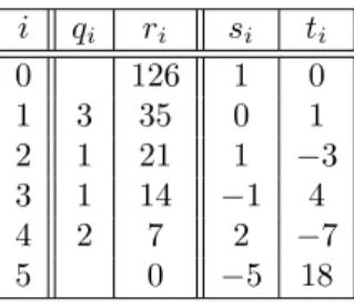
Sinceδ(ri)> δ(ri+1)≥0 fori∈N, there isl∈N0such thatrl6= 0 andrl+1= 0, hence the algorithm terminates. We haveri=sia+tibfor alli∈ {0, . . . , l+ 1}, hencer=rl =sa+tb. From ri+1 =ri−1−qiri, for all i∈ {1, . . . , l}, we get r=rl∈gcd(rl,0) = gcd(rl, rl+1) = gcd(ri, ri+1) = gcd(r0, r1) = gcd(a, b). ] Example. ForR:=Zleta:= 2·32·7 = 126 andb:= 5·7 = 35, then Table 2
shows thatd:= 7 = 2a−7b∈gcd(a, b). ]
(1.5) Theorem: Euclid implies Gauß. Any Euclidean domain is factorial.
Proof. LetR be an Euclidean domain with (monotonous) degree map δ. We first show that any 06=a∈R\R∗is a product of irreducible elements: Assuming the contrary, letabe chosen of minimal degree not having this property. Then ais reducible, hence there are b, c ∈R\R∗ such that a =bc. Thus we have δ(b)< δ(a) and δ(c)< δ(a), implying that both band c are irreducible, hence ais a product of irreducible elements, a contradiction.
In order to show uniqueness of factorizations, we next show that any irreducible element 0 6=a∈R\R∗ has the following property: Given b, c∈R such that a - banda | bc, then we have 1∈gcd(a, b), hence there are B´ezout coefficients s, t∈Rsuch that 1 =sa+tb, implying thata | sac+tbc=c.
Now leta=u·Qn
i=1pi∈R, where thepi are irreducible, n∈N0 andu∈R∗. We proceed by induction onn∈N0, where we haven= 0 if and only ifa∈R∗. Hence let n ≥ 1, and let a = Qm
j=1qj ∈ R, where the qj are irreducible and m∈N. Sincepn is irreducible, by the property proven above, we may assume thatpn | qm, hence sinceqmis irreducible, too, we inferpn ∼qm. Thus we have u0·Qn−1
i=1 pi=Qm−1
j=1 qj ∈R, for someu0∈R∗, and we are done by induction. ] (1.6) Polynomial rings. a) LetX be asymbol or indeterminate. Then the setX∗:={Xi;i∈N0}ofwordsinXbecomes a commutative monoid with respect toconcatenation given by Xi·Xj :=Xi+j, for all i, j ∈ N0, having neutral element 1 :=X0. Thus we may identify the additive monoid N0 with X∗ viaN0→X∗: i7→Xi.
LetK[X] :={[a0, a1, . . .]∈Maps(X∗, K);ai = 0 for almost alli∈N0}, where Kis a field. The mapf:X∗→K:Xi7→ai is (essentially uniquely) written as aformal sumf =P
i≥0aiXi, and is called apolynomialinX, whereai∈K is called itsi-thcoefficient.
Iff 6= 0 then deg(f) := max{i∈N0;ai 6= 0} ∈ N0 is called itsdegree, where polynomials of degree 0, . . . ,3 are called constant, linear, quadratic, and cubic, respectively, and lc(f) :=adeg(f)∈K is called its leading coefficient;
if lc(f) = 1 thenf is calledmonic.
b) We define addition on K[X] componentwise by letting (P
i≥0aiXi) + (P
j≥0bjXj) := P
k≥0(ak+bk)Xk. Similarly, we define scalar multiplication K×K[X]→K[X] componentwise by lettinga·(P
i≥0aiXi) :=P
i≥0aaiXi. ThusK[X] becomes aK-vector space, havingK-basis{1·Xi;i∈N0}, which we may identify withX∗. Hence the formal sum notation just expresses elements ofK[X] as K-linear combinations of the K-basisX∗.
We defineconvolutionalmultiplication onK[X] by letting (1·Xi)·(1·Xj) :=
(1·Xi+j), and extending K-linearly in both arguments. In other words, we have (P
i≥0aiXi)·(P
j≥0bjXj) =P
i,j≥0aibjXi+j=P
k≥0(Pk
l=0albk−l)Xk. Since X∗ is a commutative monoid, and multiplication on K fulfills associa- tivity and commutativity,K[X] becomes a commutative multiplicative monoid with neutral element 1 := 1·X0. Since arithmetic inK fulfills distributivity, this also holds for K[X]. Thus K[X] is a commutative ring, being called the (univariate) polynomial ringin X overK.
K[X] is an integral domain, such that f | g implies deg(f)≤deg(g): For 06=
f, g∈K[X] we have lc(f)6= 06= lc(g), hence fromK being an integral domain we infer thatf g6= 0, where deg(f g) = deg(f) + deg(g) and lc(f g) = lc(f)lc(g).
Table 3: Extended Euclidean algorithm inQ[X].
i qi ri si ti
0 X5−X3+ 2X2−2 1 0
1 X2−2X+ 1 X3+ 2X2+ 2X+ 1 0 1
2 13(X+ 2) 3X2−3 1 −X2+ 2X−1
3 X−1 3X+ 3 −13 (X+ 2) 13(X3−3X+ 5)
4 0 13(X2+X+ 1) −13 (X4−X3+ 2X−2)
We may considerK as a subset ofK[X] via K →K[X] : a7→a·1. Then we haveK[X]∗=K∗; in particularK[X] is not a field: We have K∗=K\ {0}= {a·X0; 06=a∈K} ⊆K[X]∗, and the additivity of degrees implies that for any 06=f ∈K[X] such that deg(f)≥1 we havef 6∈K[X]∗.
(1.7) Theorem: Polynomial division. Let f, g ∈ K[X] such that g 6= 0.
Then there are (uniquely determined) q, r ∈ K[X], called quotient and re- mainder, respectively, such thatf =qg+rwherer= 0 or deg(r)<deg(g).
Proof. Letqg+r =f =q0g+r0 where q, q0, r, r0 ∈ R[X] such thatr = 0 or deg(r) < deg(g), and r0 = 0 or deg(r0) < deg(g). Then we have (q−q0)g = r0−r, wherer0 −r = 0 or deg(r0−r)<deg(g), and where (q−q0)g = 0 or deg((q−q0)g) = deg(g) + deg(q−q0) ≥ deg(g). Hence we have r0 = r and (q−q0)g= 0, implyingq=q0, showing uniqueness.
To show existence, we may assume thatf 6= 0 and m:= deg(f)≥deg(g) :=n.
We proceed by induction onm∈N0: Letting f0 :=f−lc(f)lc(g)−1gXm−n ∈ K[X], them-th coefficient off0shows thatf0= 0 or deg(f0)< m. By induction there areq0, r0∈K[X] such thatf0 =q0g+r0, wherer0 = 0 or deg(r0)<deg(g), hencef = (q0g+r0) + lc(f)lc(g)−1gXm−n= (q0+ lc(f)lc(g)−1Xm−n)g+r0. ] (1.8) Corollary: Polynomial implies Euclid. K[X] is an Euclidean domain with respect to the degree map deg.
Thus any 0 6=f ∈ K[X] can be written uniquely as f = lc(f)·Q
p∈Ppνp(f), where νp(f)∈ N0 and P ⊆K[X] is the set of monic irreducible polynomials, being a set of representatives of the associate classes of irreducible polynomials;
we have deg(f) =P
p∈Pνp(f) deg(p)∈N0.
Example. Forf := (X3+ 2)(X+ 1)(X−1) =X5−X3+ 2X2−2∈Q[X] and g:= (X2+X+ 1)(X+ 1) = X3+ 2X2+ 2X+ 1∈Q[X] we get f =qg+r, whereq:=X2−2X+ 1∈Q[X] and r:= 3X2−3∈Q[X]. Table 3 shows that d:=X+ 1∈gcd(f, g), whered=−19 (X+ 2)·f+−19 (X4−X3+ 2X−2)·g. ]
(1.9) Evaluation. a)Letϕ:K→S be a ring homomorphism into a ringS, such thatϕ(a)z=zϕ(a), for alla∈Kandz∈S. Then forz∈Swe have the as- sociatedevaluation mapϕz:K[X]→S:f =P
i≥0aiXi 7→P
i≥0ϕ(ai)zi=:
fϕ(z); in particular, forϕ= idK we just writef(z) =P
i≥0aizi.
Thenϕzis a ring homomorphism: We haveϕz(1) =ϕ(1) = 1, additivityϕz(f+ g) =ϕz(P
i≥0(ai+bi)Xi) =P
i≥0ϕ(ai+bi)zi=P
i≥0ϕ(ai)zi+P
i≥0ϕ(bi)zi = ϕz(f) +ϕz(g), and multiplicativity ϕz(f g) = ϕz(P
i≥0(Pi
j=0ajbi−j)Xi) = P
i≥0(Pi
j=0ϕ(aj)ϕ(bi−j))zi= (P
i≥0ϕ(ai)zi)·(P
i≥0ϕ(bi)zi) =ϕz(f)ϕz(g).
b) For f ∈ K[X] we get the associated polynomial map fbϕ: S → S:z 7→
fϕ(z); in particular, forϕ= idK we just writefb: K→K:z7→f(z).
Since S is a ring, the set Maps(S, S) also becomes a ring with pointwise addition F +G:S → S: z 7→ F(z) +G(z) and multiplication F ·G: S → S: z 7→ F(z)G(z), neutral elements being the constant maps S → S: z 7→ 0 andS→S:z7→1, respectively.
Hence, since the evaluation mapϕz:K[X]→S is a ring homomorphism for all z∈S, we infer thatϕ:b K[X]→Maps(S, S) :f 7→fbϕ is a ring homomorphism.
c)Iffϕ(z) = 0 thenz∈S is called aroot orzerooff inS.
Forϕ= idK, an elementa∈Kis a root off ∈K[X], if and only if (X−a) | f: Writingf =q·(X−a) +r, where r= 0 or deg(r)<deg(X −a) = 1, that is r∈K, we getr=f(a)−q(a)·(a−a) =f(a).
Thena∈K is called a root off 6= 0 of multiplicityνa(f) :=νX−a(f)∈N0; note that (X−a)∈ P. FromP
a∈Kνa(f)≤deg(f) we conclude thatf 6= 0 has at most deg(f)∈N0roots in K, counted with multiplicity.
The fieldKis called algebraically closedif any polynomial inK[X]\K has a root in K, or equivalently if P ={X−a∈K[X];a∈K}. By theFunda- mental Theorem of Algebra [Gauß, 1801]the field of complex numbersC is algebraically closed.
The mapϕb:K[X]→Maps(K, K) is injective if and only ifKis infinite; in this case we may identify polynomials and polynomial maps:
If K is finite, then for f := Q
a∈K(X −a) ∈ K[X] we get f(z) = 0 ∈ K for all z ∈ K, thus fb=b0 ∈ Maps(K, K). If K is infinite, then for f, g ∈ K[X]
such thatfb=bg∈Maps(K, K) we conclude thatf −g has all infinitely many elements ofK as roots, implying thatf−g= 0∈K[X]. ]
2 Eigenvalues
(2.1) Similarity. a)LetK be a field. MatricesA, D∈Kn×n, wheren∈N0, are calledsimilar, if there isP ∈GLn(K) such thatD=P−1AP. Similarity is an equivalence relation, the equivalence classes are calledsimilarity classes.
The matrixAis calleddiagonalisable, if it is similar to a diagonal matrix. The matrixA is called triangularisable, if it is similar to a (lower) triangular matrix, that is a matrixM := [bij]ij ∈Kn×n such thatbij = 0 for allj > i∈ {1, . . . , n}; in particular a diagonalisable matrix is triangularisable.
Triangularisability is equivalent to requiring that A is similar to an upper triangular matrix, that is a matrixN := [cij]ij ∈Kn×n such thatcij= 0 for alli > j∈ {1, . . . , n}: LettingP := [aij]ij∈Kn×n, whereaij := 1 if and only if i+j=n+ 1, andaij := 0 elsewise, for any lower triangular matrixM ∈Kn×n the matrixP−1N P ∈Kn×n is an upper triangular.
b)LetV be aK-vector space such that dimK(V) =n. Thenϕ, ψ∈EndK(V) are called similar, if there are K-bases B and C of V such that MBB(ϕ) = MCC(ψ)∈Kn×n. SinceP :=MBC(id)∈GLn(K) andMCC(ψ) =P−1·MBB(ψ)·P this is equivalent to saying thatMBB(ϕ) andMBB(ψ) are similar.
Moreover,ϕis calleddiagonalisableor triangularisable, ifMBB(ϕ) is diago- nalisable or triangularisable, respectively, for some, hence anyK-basisB⊆V. (2.2) Eigenvalues. a)Let K be a field, let V be a K-vector space, and let ϕ ∈ EndK(V). Then a ∈ K is called an eigenvalue of ϕ, if there is an eigenvector06=v∈V such thatϕ(v) =av.
Given a∈K, we haveϕ−a·id ∈EndK(V) as well, hence we have Ta(ϕ) :=
ker(ϕ−a·id) ={v∈V;ϕ(v) =av} ≤V, being called the associatedeigenspace ofϕ. Hence Ta(ϕ)\ {0} is the associated set of eigenvectors ofϕ.
Lettingγa(ϕ) := dimK(Ta(ϕ))∈N0
∪ {∞}. be the associatedgeometric mul- tiplicity, ais an eigenvalue ofϕ if and only ifγa(ϕ)≥1. In particular, from ker(ϕ) =T0(ϕ) we infer thatϕis injective if and only if 0 is not an eigenvalue.
b)LetI be a set, and let [ai∈K;i∈ I] be pairwise different eigenvalues ofϕ.
Then any sequence [vi∈Tai(ϕ)\ {0};i∈ I] is K-linearly independent:
LetJ ⊆ Ibe finite, where we may assume thatJ ={1, . . . , n}for somen∈N0. We proceed by induction, the casen= 0 being trivial: Letb1, . . . , bn ∈Ksuch that Pn
i=1bivi = 0. Hence we have 0 =ϕ(Pn
i=1bivi) =Pn
i=1aibivi, and thus 0 = an ·Pn
i=1bivi−Pn
i=1aibivi = Pn−1
i=1(an −ai)bivi. By induction we get (an−ai)bi= 0, andan−ai6= 0 impliesbi = 0, for alli∈ {1, . . . , n−1}. Thus
finallyvn6= 0 impliesbn= 0. ]
Example. Let C∞(R) :={f:R→R;f smooth} ≤Maps(R,R), and let ∂x∂ ∈ EndR(C∞(R)), adifferential operator. Then for a:R→R:x7→exp(ax), where a ∈ R, we have ∂x∂ (a) =aa. Hence a is an eigenvalue of ∂x∂ , having a ∈ C∞(R) as an eigenvector, and [a ∈ C∞(R);a ∈ R] is R-linearly inde- pendent. But note that, since all non-trivial (finite) R-linear combinations of [a∈C∞(R);a∈R] are unbounded maps, this is not anR-basis ofC∞(R). ] c)The above behaviour of eigenvectors can be rephrased in terms of the follow- ing general notion: LetI be a set, and letUi ≤V for alli∈ I. Then the sum
U :=P
i∈IUi ≤V is called direct, if any sequence [vi ∈Ui\ {0};i∈ I, Ui 6=
{0}] isK-linearly independent; we writeU =L
i∈IUi. Thus we haveU =L
i∈IUi if and only if any v∈U can be written essentially uniquely as aK-linear combinationv=P
j∈J ajvj, whereJ ⊆ I is finite, and vj ∈ Uj for all j ∈ J. In other words, we have U = L
i∈IUi if and only if Ui∩(P
j6=iUj) ={0}, for alli∈ I.
Moreover, if I is finite and the Ui are finitely generated K-vector spaces, then iterating the dimension formula for subspaces, saying that dimK(Ui) + dimK(Uj) = dimK(Ui +Uj) + dimK(Ui∩Uj) for all i, j ∈ I, implies that U =L
i∈IUi if and only if dimK(U) =P
i∈IdimK(Ui).
For example, if [vi∈V;i∈ I] is aK-basis ofV, then we haveV =L
i∈IhviiK. And coming back to eigenspaces, letting U := P
a∈KTa(ϕ) ≤ V, we have U =L
a∈KTa(ϕ) =L
a∈K,γa(ϕ)≥1Ta(ϕ).
(2.3) Eigenvalues of matrices. If dimK(V) = n∈N0, then choosing aK- basis B ⊆ V and identifying V → Kn×1: v 7→ MB(v) translates notions for ϕ∈EndK(V) into those ofMBB(ϕ)∈Kn×n:
The eigenvalues and eigenvectors of a matrixA∈Kn×n are defined to be those ofϕA:Kn×1→Kn×1:v7→Av. Hencea∈K is an eigenvalue ofAif and only ifTa(A) := ker(A−aEn)6={0}. For the associated geometric multiplicity we haveγa(A) := dimK(Ta(A)) = dimK(ker(A−aEn)) =n−rk(A−aEn). Since for P∈GLn(K) we have rk(P−1AP−aEn) = rk(P−1(A−aEn)P) = rk(A−aEn), we conclude that geometric multiplicities only depend on similarity classes.
The matrixAis diagonalisable if and only if there is a K-basis{v1, . . . , vn} ⊆ Kn×1 consisting of eigenvectors of A. In this case, for P := [v1, . . . , vn] ∈ GLn(K) we have P−1AP = D := diag[a1, . . . , an] ∈ Kn×n. Since γa(A) = dimK(Ta(D)) = |{i∈ {1, . . . , n};ai =a}|, for alla∈K, we conclude that the (not necessarily pairwise different) diagonal entries {a1, . . . , an} are precisely the eigenvalues ofA, each occurring with multiplicity γa(A). The eigenvalues together with their geometric multiplicities are called thespectrumofA.
Since the various eigenspaces ofA form a direct sum, we conclude that A has at mostnpairwise different eigenvalues. In this case, picking associated eigen- vectors, we infer thatKn×1 has aK-basis consisting of eigenvectors ofA, that isAis diagonalisable, and we haveγa(A)≤1 for alla∈K.
Example. We reconsider the reflection given in (0.6): In terms of matrices, let A :=
. 1 1 .
∈ R2×2. Then for the vectors v1 := [1,1]tr ∈ R2×1 and v2:= [−1,1]tr∈R2×1we haveA·v1=v1andA·v2=−v2, that is they are are eigenvectors ofAwith respect to the eigenvalues 1 and−1, respectively. Letting P :=
1 −1
1 1
∈GL2(R) we have P−1 := 12·
1 1
−1 1
, and indeed P−1AP =
1 2·
1 1
−1 1
· . 1
1 .
· 1 −1
1 1
= 1 .
. −1
=:D. ThusAis diagonalisable, where {±1} are the eigenvalues ofA, both occurring with geometric multiplicity 1. ] (2.4) Characteristic polynomials. LetK be a field and let A ∈ Kn×n ⊆ K[X]n×n, wheren∈N0. Then XEn−A∈K[X]n×n is called thecharacter- istic matrixassociated withA, andχA:= det(XEn−A)∈K[X] is called the characteristic polynomialofA.
Note that we have defined determinants only for matrices over fields. But the definition given in (0.2) makes perfect sense in the more general setting of ma- trices over a commutative ring. Moreover, it can be checked that the basic properties, such as the arithmetical rules given in (0.2), multiplicativity in The- orem (0.3), and Laplace expansion in Theorem (0.4) continue to hold.
ThenχA6= 0 is monic of degree deg(χA) =n, and we haveχA(0) = det(−A) = (−1)n·det(A) ∈K. For example, for D := diag[a1, . . . , an] ∈Kn×n we have χD= det(XEn−D) =Qn
i=1(X−ai)∈K[X].
Moreover, since for P ∈ GLn(K) we haveχP−1AP = det(XEn−P−1AP) = det(P−1(XEn−A)P) = det(XEn−A) =χA ∈K[X], we conclude thatχA∈ K[X] only depends on the similarity class ofA.
IfV is a finitely generatedK-vector space andϕ∈EndK(V), choosing aK-basis B⊆V yields thecharacteristic polynomialχϕ:=χMB
B(ϕ)∈K[X].
b)Given a∈K, the multiplicity νa(A) :=νa(χA) = νX−a(χA)∈N0 is called the associatedalgebraic multiplicity. Hence we haveP
a∈Kνa(A)≤n, and algebraic multiplicities only depend on the similarity class ofA.
Hence a is an eigenvalue ofA, that is Ta(A) = ker(A−aEn)6={0}, in other wordsγa(A)≥1, if and only if det(aEn−A) = (−1)n·det(A−aEn) = 0, or equivalentlyχA(a) = 0, that isais a root ofχA, in other wordsνa(A)≥1.
In particular, this again shows that A has at most n pairwise different eigen- values, in which case we have νa(A) ≤ 1 for all a ∈ K. Moreover, if K is algebraically closed andn≥1 thenAhas an eigenvalue.
c)For anya∈K we haveνa(A)≥γa(A):
LetP := [v1, . . . , vn]∈GLn(K) be aK-basis ofKn×1 such that [v1, . . . , vm] is a K-basis of Ta(A)≤Kn×1, wherem:=γa(A)∈ {0, . . . , n}. ThenP−1AP = D ∗
0 A0
, whereD= diag[a, . . . , a]∈Km×mandA0∈K(n−m)×(n−m), yields χA= det
XEm−D ∗ 0 XEn−m−A0
= det(XEm−D)·det(XEn−m−A0) = χD·χA0 = (X−a)m·χA0∈K[X], hence we inferνa(A)≥m. ] In particular, sinceγa(A) = 0 if and only if νa(A) = 0, we infer thatνa(A) = 1 entailsγa(A) = 1.
(2.5) Diagonalisability. LetK be a field and letA∈Kn×n, where n∈N0. ThenAis diagonalisable if and only ifχA∈K[X] splits into linear factors and for alla∈K we have νa(A) =γa(A):
If A = diag[a1, . . . , an] ∈ Kn×n, then we have χA = Qn
i=1(X−ai) ∈ K[X], whereνa(A) =|{i∈ {1, . . . , n};ai =a}|=γa(A), for alla∈K.
Conversely, if χA =Qs
i=1(X −ai)νai(A) ∈ K[X], where {a1, . . . , as} ⊆ K are the eigenvalues ofAwith multipliticitiesνai(A) =γai(A)∈N, for somes∈N0, thenPs
i=1dimK(Tai(A)) =Ps
i=1γai(A) =Ps
i=1νai(A) = deg(χA) =n, hence Ls
i=1Tai(A) being a direct sum, we inferLs
i=1Tai(A) =Kn×1, implying that there is aK-basis consisting of eigenvectors ofA, that isAis diagonalisable. ] Note that the condition on the equality of algebraic and geometric multiplicities is non-trivial only for the eigenvalues ofA. Moreover, ifAhasnpairwise differ- ent eigenvalues, thenχAsplits into linear factors, and we haveνa(A) =γa(A) = 1 for all eigenvaluesaofA, hence we recover the fact that Ais diagonalisable.
Example. i) Let A :=
. 1 1 .
∈ R2×2, that is we reconsider the reflection given in (0.6). Then we have XEn−A =
X −1
−1 X
∈ R[X]2×2, thus χA = X2−1 = (X−1)(X+ 1)∈R[X]. HenceAhas the eigenvalues{±1} ⊆R, where ν±1(A) = γ±1(A) = 1. We have ker(A−E2) = h[1,1]triR and ker(A+E2) = h[−1,1]triR. Hence picking the vectors indicated we indeed recover the C-basis consisting of eigenvectors chosen above.
ii) Let A :=
cos(ω) −sin(ω) sin(ω) cos(ω)
∈ R2×2, that is we reconsider the rotation with respect to the angle ω ∈ R given in (0.6); in particular, the rotation with respect to the angle π2 is given by
. −1
1 .
. Then we have XEn−A = X−cos(ω) sin(ω)
−sin(ω) X−cos(ω)
∈ R[X]2×2 ⊆ C[X]2×2, from which we get χA = X2−2 cos(ω)X+ 1∈R[X]⊆C[X], having rootsa± := cos(ω)±i·sin(ω) = exp(±iω) ∈ C. Hence we have a± ∈ R if and only if ω = kπ, where k ∈ Z; in this case we have A= (−1)k·E2, which already is a diagonal matrix, and χA= (X−(−1)k)2, thusν(−1)k(A) =γ(−1)k(A) = 2.
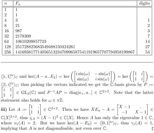
Ifω6∈πZthena±∈C\R. ThusχA∈R[X] is irreducible, andAdoes not have any eigenvalues inR, in particularAis not diagonalisable. Note that this is the algebraic counterpart of the geometric observation that for these rotations there cannot possibly exist non-zero vectors being mapped to multiples of themselves.
Still assumingω6∈πZ, fromχA= (X−a+)(X−a−)∈C[X] wherea+6=a−, we infer thatAhas the eigenvalues{a±} ⊆C, whereνa±(A) =γa±(A) = 1, henceA is diagonalisable overC, being similar to diag[a+, a−]∈C2×2. More precisely, we have ker(A−a+E2) = ker
−isin(ω) −sin(ω) sin(ω) −isin(ω)
= ker i 1
i 1
=
Table 4: Fibonacci numbers.
n Fn digits
1 1
2 1
4 3 1
8 21 2
16 987 3
32 2178309 7
64 10610209857723 14
128 251728825683549488150424261 27
256 141693817714056513234709965875411919657707794958199867 54
h[i,1]triC and ker(A−a−E2) = ker
isin(ω) −sin(ω) sin(ω) isin(ω)
= ker 1 i
1 i
= h[1, i]triC; thus picking the vectors indicated we get the C-basis given by P :=
i 1 1 i
∈ GL2(C) and P−1AP = diag[a+, a−] ∈ C2×2. Note that the latter statement also holds forω∈πZ.
iii) LetA :=
1 . 1 1
∈C2×2. Then we have XEn−A =
X−1 .
−1 X−1
∈ C[X]2×2, thus χA= (X−1)2∈C[X]. HenceAhas only the eigenvalue 1∈C, where ν1(A) = 2. But we have ker(A−E2) = h[0,1]triC, thus γ1(A) = 1, implying thatAis not diagonalisable, not even overC. ] (2.6) Example: Fibonacci numbers. The following problem was posed in the medieval book ‘Liber abbaci’ [Leonardo da Pisa ‘Fibonacci’, 1202]:
Any female rabbit gives birth to a couple of rabbits monthly, from its second month of life on. If there is a single couple in the first month, how many are there in monthn∈N?
Hence let [Fn ∈ N0;n∈N0] be thelinear recurrent sequenceof degree 2 given byF0 := 0 and F1 := 1, and Fn+2 := Fn+Fn+1 forn ∈ N0. Thus we obtain the sequence ofFibonacci numbers, see also Table 4:
n 0 1 2 3 4 5 6 7 8 9 10 11 12 13 14 15
Fn 0 1 1 2 3 5 8 13 21 34 55 89 144 233 377 610 To find a closed formula for the Fibonacci numbers, and to determine their growth behavior, we proceed as follows: LettingA :=
. 1 1 1
∈R2×2 we have
![Table 3: Extended Euclidean algorithm in Q [X]. i q i r i s i t i 0 X 5 − X 3 + 2X 2 − 2 1 0 1 X 2 − 2X + 1 X 3 + 2X 2 + 2X + 1 0 1 2 1 3 (X + 2) 3X 2 − 3 1 −X 2 + 2X − 1 3 X − 1 3X + 3 −1 3 (X + 2) 13 (X 3 − 3X + 5) 4 0 1 3 (X 2 + X + 1) −13 (X 4 − X 3 +](https://thumb-eu.123doks.com/thumbv2/1library_info/5270029.1674988/13.918.199.717.245.352/table-extended-euclidean-algorithm-q-x-x-x.webp)