Commission-Based Pay –
Three Essays on German Insurance Tied Agents
Inauguraldissertation zur
Erlangung des Doktorgrades der
Wirtschafts- und Sozialwissenschaftlichen Fakult¨at der
Universit¨at zu K ¨oln
2009
vorgelegt von
Dipl.-Math. techn. Robert Widura aus
Georgsmarienh ¨utte
Referent: Prof. Dr. Dirk Sliwka
Korreferent: Prof. David A. Jaeger, Ph.D.
Tag der Promotion: 18. Dezember 2009
Contents
1 Introduction 4
2 The Relation Between Incentives, Effort and Performance 11
2.1 Introduction . . . 11
2.2 The Model . . . 15
2.2.1 Theoretical Predictions . . . 15
2.2.2 Predictions from Simulated Data . . . 24
2.3 Empirical Results . . . 30
2.3.1 Data Description . . . 30
2.3.2 Effect of Effort Allocation on Performance . . . 33
2.3.3 Effect of Incentives on Effort Allocation . . . 35
2.3.4 Robustness . . . 39
2.4 Discussion and Conclusion . . . 41
2.5 Appendix to Chapter 2 . . . 43
3 The Effect of Tenure, Industry- and General-Experience on Com-
pensation 46
3.1 Introduction . . . 46
3.2 The Model . . . 53
3.3 Empirical Results . . . 57
3.3.1 Data Description . . . 57
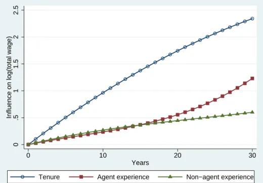
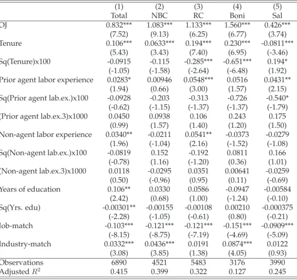
3.3.2 Effect of Experience on Total Wage . . . 61
3.3.3 Effect of Experience on Sub-Components of Wage . . 66
3.3.4 Robustness . . . 72
3.4 Discussion and Conclusion . . . 75
3.5 Appendix to Chapter 3 . . . 77
4 Reference-Point Dependency of Pay Satisfaction 84 4.1 Introduction . . . 84
4.2 The Model . . . 89
4.3 Methodological Background . . . 91
4.4 Empirical Results . . . 95
4.4.1 Data Description . . . 95
4.4.2 Effect of Absolute Compensation on Satisfaction . . . 97
4.4.3 Reference-Point Dependent Satisfaction . . . 103
4.4.4 Robustness . . . 108
4.5 Discussion and Conclusion . . . 109
4.6 Appendix to Chapter 4 . . . 111
References 117
Chapter 1
Introduction
(Calvin and Hobbes, Watterson (2006))
This comic-strip byCalvin and Hobbesis an example for the intrinsic effort- allocation of an ”agent” not always being in line with the desired alloca- tion by the ”principal”. The basic but crucial question of how to design an incentive scheme that endorses a certain agent behavior has given rise to extensive economic research in the past. To understand and describe the influence of incentives properly, the individual characteristics of each worker (e.g., ability, age, labor-market experience) have to be considered.
Cognitive and motivational mechanisms also play an important role in determining how a certain level of compensation translates into job- and pay-satisfaction.
Figure 1.1: Guiding framework of my thesis (based on Bonner & Sprinkle (2002))
Figure 1.1 summarizes this diverse set of effects and mechanisms, based on a framework suggested by Bonner & Sprinkle (2002). My thesis is struc- tured along this framework and consists of three main building blocks.
The first of these is the relationship between incentives, allocation of ef- fort, and task performance. Second, I will analyze how person variables, i.e., different forms of labor-market experience, influence the agent’s per- formance. Finally, I discuss the effect of compensation on agent satisfac- tion, using a model of expectancies and reference-point dependent utility.
I discuss the findings of each of the three chapters in more detail below, after giving a brief introduction to the data-set I use throughout my work.
The data is on German insurance tied agents1 and was collected in the first half of 2006. It is based on an online questionnaire among German insurance companies. A total of 9,386 insurance tied agents from 10 large German insurance companies participated in the survey (for more infor-
1 An ”official” definition can be found in the German commercial code (HGB,§84 Abs.
1), which defines tied agents as ”independent tradesmen that act as an agent for another company. ”Independent” means someone, who is generally free to decide which tasks to perform and how to spend his time” (see also Heinz (1999))
mation regarding set-up and concept of the questionnaire, see also Vogler (2009)). The data was sanitized, meaning that both the agents and the companies remained anonymous. As the level of information provided differs among the ten companies, not all observations could be used in the analyses, depending on the research question under consideration. Each chapter therefore contains a section in which I describe the subset of data used for the specific analysis. Overall, though, the findings presented in this work are based on a comparably large number of observations and therefore can be said to be representative.
One major difference to most of the other works that have been published in the past is that this focuses on one single industry in one country. The concentration on this specific industry and occupation, enables us to study in detail the effects under consideration due to the special nature of the compensation scheme of insurance agents, which is almost entirely vari- able, based on commission rates. Therefore, a clear link exists between performance and pay. This is a big advantage compared to other stud- ies that cover a broad range of occupations and industries. As already stressed by Goette et al. (2004), an environment in which workers are free to choose when and how much to work and where a salient relationship between their effort and their income exists, is the ideal context in which to test the standard, neoclassical model of intertemporal labor supply. In this sense, I do not consider insurance tied agents an artificial case, but rather a job and industry that is perfectly suited for economic research.
As we will refer to the compensation system applicable to German insur- ance tied agents frequently in the subsequent chapters, I will now briefly present the general set-up of their compensation system.
The four components of the agents compensation are (i) new business commissions, (ii) recurring commissions, (iii) bonification and (iv) fixed salary and subsidies.2 The insurance company pays these components to the agent, with the commissions directly related to new business gen- erated and the total portfolio managed, whilst the bonification is paid for
2 I will refer to these four components also as NBC, RC, Boni and Sal throughout the text, especially in the column-headers of regression tables
achieving or surpassing previously agreed goals. The fixed salary/subsidies component is usually paid only in the first couple of years after an agent joins the insurer, in order to help the agent sustain a minimal level of earnings (see Beenken (2003) and Damm (1993)). Apart from these purely monetary incentives, there can also be non-monetary rewards, e.g., travel vouchers, a watch, or some form of public recognition. Although there is evidence that these non-financial rewards can be very motivating, as they conspicuously recognize the agent’s achievements (Dorfman (1976)), this type of bonification is outside the scope of this work (in line with Coughlan & Narasimhan (1992)). More information on the compensation systems of German insurance agents can be found in Cummins & Doherty (2006) (who focus on non-tied insurance intermediaries), Cupach & Car- son (2002), Heinz (1999), Ludwig (1994) and Dorfman (1976).
I will now give a brief outline of the chapters of this thesis, including the main findings of the analyses.
Chapter 2 focuses on the question of how incentives can influence agents’
time allocation and whether they can lead to a change in performance.
Many recent studies have suggested that incentives matter, and that piece- rates are the best way to endorse the desired behavior (see e.g., Shearer (2004), Paarsch & Shearer (2000), Lazear (2000) or Lazear (1986)). Empiri- cal evidence that supports this hypothesis, however, is scarce (see Bonner et al. (2000)). Alongside the problem of if and how incentives increase the amount of effort exerted by the agent, there is also the question of how the effort is allocated. A common hypothesis among practitioners is that there is always a trade-off between acquiring new customers and caring for ex- isting ones (see Albers (2006), Cupach & Carson (2002), Albers (1996) or Sautter (1980)). I use the concept of a multi-task model based on the sem- inal work by Holmstrom & Milgrom (1991) to describe this trade-off be- tween selling and customer care. Initially, I develop a simple one-period multi-task model and derive hypotheses regarding the influence of effort allocation on performance and how commission rates can be used to steer this allocation. This model is then extended to a 2-period setting where we include the intertemporal dependencies arising from the portfolio-effect
(i.e., that extending effort on selling also increases future recurring com- missions and that a higher retention of customers via an increase in cus- tomer care effort is also beneficial in the next period). We revisit our hy- potheses from the one-period model using simulated data and find that they generally hold for the 2-period case. Second, I test the hypotheses using data on auto insurance sales of three German insurance companies.
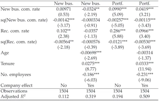
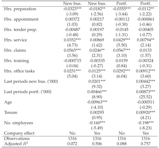
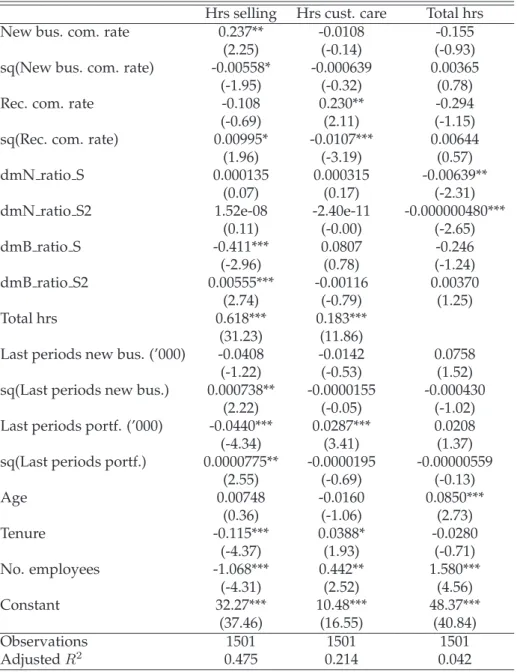
I find a significant positive effect of the time spent on customer care ac- tivities both on the portfolio size and new business production. The new business commission rate has a positive effect on selling and a negative ef- fect on customer care time. The results for the recurring commission rate are mixed.
In Chapter 3, I turn towards the influence of individual characteristics of each worker. The human capital theory is well-known and seeks to explain the relationship between experience and pay, stating that more experience makes the employee more valuable and should thus lead to higher wages.
Previous research has cast some doubts on this simple relationship and suggested that the type of experience needs to be differentiated from the total sum of experience. The analysis presented here leans on the work by Parent (2000), who found that three categories of experience can be distin- guished: industry-specific, job-specific and general labor-market experi- ence (the works by Kambourov & Manovskii (2009), Poletaev & Robinson (2008) and Gibbons & Waldman (2006) suggest an even finer differenti- ation into occupational-, skill- or task-specific experience, respectively).
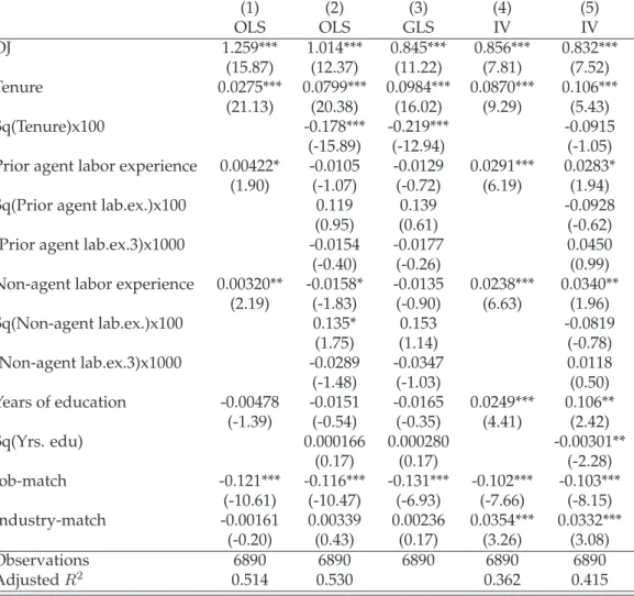
Based on the standard wage model, I test the influence of experience us- ing the data on tied agents. I find both the expected strong effect of tenure on pay due to the special structure of agent compensation in this industry, and that general- and industry-specific labor market experience also have positive effects. The latter deviate is dependent on the agent’s tenure: it is strong for agents with low tenure, but becomes rather weak or even neg- ative for high-tenure agents. A detailed look into the effects on different compensation components reveals a high degree of diversity in the size and direction of the experience-related influence on wage. By applying an instrumental variable (IV) approach (based on Altonji & Shakotko (1987))
and introducing proxy variables for the job- and industry-match, the chap- ter also contributes to the discussion regarding the omitted-variable bias that can arise from using simple OLS instead of IV.
Finally, Chapter 4 discusses the motivational aspects of compensation.
Camerer et al. (1997) found (using data on taxicab drivers) that theexpected wage acts as a reference-point and that performance drops after that target is met. Similarly, Groot & van Maassen den Brink (1999), found that the positive effect of higher wages on job satisfaction wears off after some time (called ”preference drift”). Recent works have found such a reference- dependent utility not only in employer-employee relationships but also in other areas of public life (see Clark et al. (2009), Luttmer (2005) and Stutzer (2004)). One of the most often analyzed phenomena in the context of reference points is ”loss aversion”: people usually feel that a loss re- duces their utility far more than a comparable gain would increase it (see Fehr & Goette (2007), Goette et al. (2004), Tversky & Kahneman (1991) and Kahneman & Tversky (1979)). Based on this line of thought, I present em- pirical evidence for the existence of a reference-point for satisfaction with compensation. Information on the satisfaction (both with pay, and over- all) of the tied agents is used to test the hypotheses. An ordered probit regression and a subsequent analysis of the marginal effects is applied to investigate the influence of compensation on the satisfaction score. I find a relationship between the agents’ deviation from peer-group compensation and their satisfaction with pay. Surprisingly, the analysis shows a positive relation with satisfaction for deviations above the peer-group median but no statistically significant relation for deviations below the median. These results run contrary to the common notion of loss aversion presented in other publications. In line with previous work, no relation is found be- tween compensation and overall satisfaction.
Overall, the results as presented in the following three chapters support the notion that there are many influencing factors in the context of pay and performance. Due to the analysis of one single job and industry, it is possible to combine different theories that have been proposed in the past to explain many aspects of human behavior. Further research is needed
to understand in depth how the findings translate to other industries and jobs and how social (non-quantitative) preferences may interact with the evidence presented here.
Chapter 2
The Relation Between Incentives, Effort and Performance
2.1 Introduction
A basic assumption in principal-agent problems is that compensation sys- tems reward the agent for his output and provide a premium for the risk he accepts. If there is only one task the agent can potentially perform, then the challenge for the principal is to provide incentives so that the amount of effort exerted by the agent is maximized (assuming that the effort effi- ciency is unchanged). In such situations, piece rates are generally found to be superior to fixed wages (e.g., Shearer (2004), Paarsch & Shearer (2000), Lazear (2000), or Lazear (1986)). Similar results were already obtained and summarized by Prendergast (1999) so it seems reasonable to assume that agents do respond to incentives.
Intuition would suggest that higher incentives lead to higher effort and therefore higher performance, but there is a lack of empirical evidence and results of laboratory studies have been quite mixed. Bonner et al. (2000) state that only half of the studies analyzed showed a significant positive
effect of incentives on performance (a similar result was also found by Camerer & Hogarth (1999)). Gneezy & Rustichini (2000) found a positive effect of higher compensation on performance relative to lower pay (but the overall performance level may be lower because of the introduction of compensation, i.e., motivation crowding out, see also Sliwka (2003)).
Camerer et al. (1997) on the other hand find a negative effect of wage in- crease on the working hours of cab drivers. The studies by Pritchard &
Leo (1973) and Tomporowski et al. (1993) also suggest a negative correla- tion between incentives and performance.
Recent research has presented an agent-specific, preference-based solution to those counter-intuitive results. Fehr & Goette (2007) argue that loss- averse agents have a reference income level, and failure to reach this level is experienced as a loss (see also Chapter 4 where I investigate the exis- tence of a reference-point in the case of insurance tied agents). On the other hand, the marginal utility of income above the reference-point decreases discontinuously. As a consequence, one could argue that after incentives are increased, this reference-point is achieved with even less effort and thus the overall performance drops. Fehr & Goette (2007) find that in the case of bike messengers (who are paid on a commission-only basis), effort duration increases whilst the effectiveness decreases. Although the overall performance still increased in this example, these findings point towards potential negative effects of an increase of incentives. In general, it must be said that the effect of the incentive changes seem to depend heavily on the nature of the task to be performed (see Camerer & Hogarth (1999)).
A recent theory to explain the rather weak relation between incentives and performance uses the concept of ”fairness”. Fehr et al. (2009) argue that a wage increase leads to an increased effort only if the wage is perceived as fair (see also Akerlof & Yellen (1990)). Similarly, MacLeod (2007) suggests that fairness may be more important than pure profit maximization.
These models, although already quite instructive, lack an important link to reality: in modern work environments, the agent rarely has only one task to perform; in most cases, workers are in charge of a broad variety of tasks.
Thus, in contrast to the one-task situation, where the emphasis is mainly
put on effort duration, there is now an additional challenge to influence the direction of effort (see Bonner & Sprinkle (2002)). This may lead to incentives that increase the effort duration, but shift the effort direction to- wards those tasks that can be clearly measured (Br ¨uggen & Moers (2007), Fehr & Schmidt (2004)).
As outlined by Holmstrom & Milgrom (1991), the multi-task approach can be applied to production workers as well as to teachers and many other jobs. To my knowledge, there is only limited empirical evidence from real data (i.e., not from laboratory experiments) on how incentives influ- ence the allocation of time and effort among different tasks. One of the few works regarding effort direction comes from Brickley & Zimmerman (2001) who analyzed the effect of a change in organizational incentives on the teaching ratings and the research output at a top-tier business school.
They find that, after putting more emphasis on teaching ratings, the over- all score in the classroom evaluations went up whilst the average research output went down.
I contribute to this new empirical field first by developing a model that accounts for repeated interactions between the agent and customers over multiple periods and secondly by analyzing the effect of varying incentive levels on the effort duration and direction using data on German insurance agents. As already described in Chapter 1, the largest component of vari- able compensation is commission that is paid for (i) new contracts sold by the agent and (ii) customers with a multi-year contract that remain with the insurance company without cancelation of their policy within this pe- riod. Furthermore, depending on the overall performance and the targets set by the Insurance company, a bonification may be paid out at the end of the accounting period. This bonification can be either a cash amount or a non-cash reward. There is evidence that non-financial rewards can be very motivating, as they conspicuously give the recipient recognition that they have met their performance objectives (Dorfman (1976)), this type of bonification is outside the scope of this work.
I focus on commissions, as they account for more than 80%, on average, of the agent’s total annual compensation (see also Damm (1993)). As com-
mission rates vary significantly between an insurer’s different products, I focus on product-specific data. I use auto insurance products as they can be assumed to be fairly standardized and thus the data from different insurance companies can be used without large company-specific differ- ences in the products.
A common hypothesis among practitioners is that there is always a trade- off between acquiring new customers and caring for existing ones. As outlined for example by Sautter (1980), it is either that agents lose sight of their existing customers in order to have more time to sell products to new ones (see Cupach & Carson (2002) or Albers (1996)) or that those agents with a broad customer base stop writing new business as they are already well paid by the recurring commissions (see Albers (2006)). Based
Figure 2.1: Framework for the effects of monetary incentives on effort and task performance (see also Figure 1.1)
on Figure 1.1, Figure 2.1 shows the different quantities I will analyze in this chapter and gives a first indication of the potential causal relations based on the literature review. I will treat the new business and recurring commission rates as the only steering instruments the principal has avail- able. Companies seem to be able to influence their agents’ time allocation between three tasks: customer care, selling and administration.3 Finally, the way the agent splits his time between the tasks should influence his performance, which I measure in terms of new business production and portfolio development.
Understanding the causal relation between incentives, effort allocation and performance has the potential to improve the effectiveness of com-
3 I will disregard the impact of effort spent on administration in the model, as I assume that the agent cannot directly influence the amount of administrative work to be performed. In the empirical results, I control for administrative tasks but focus on interpreting the effects from customer care and selling
pensation schemes, not only in the sense of efficiency gains for the princi- pal but also in terms of the agent’s well-being. Survey results by Graf &
Keese (2000) show that 43% of agents perceive their current compensation system as ”unfair”.
In the next section, I develop a formal model and derive specific hypothe- ses regarding the different effects just discussed using both closed-form solutions (2.2.1) and simulated data (2.2.2). In Section 2.3, I give a brief introduction into the data-set (2.3.1), test the hypotheses (2.3.2 and 2.3.3) and discuss the robustness of the results (2.3.4). Section 2.4 summarizes the findings and concludes.
2.2 The Model
2.2.1 Theoretical Predictions
In this section, I develop a model to derive the optimal effort allocation of an agent that has the choice between multiple tasks. The model specifica- tion leans heavily on the seminal work by Holmstrom & Milgrom (1991).
As in their work, I also focus on a linear-contract, normal-noise, CARA4- preference setting. Based on the theoretical results, I formulate hypothe- ses regarding the influence of effort and commission rates on performance that I test in Section 2.3 with the data-set. I am interested in the optimal effort allocation of the agent, so I do not discuss the principal’s problem here and assume that the commission rates are externally set.
I start with a 1-period model (assuming that the agent is completely my- opic). In the second stage, I extend the model into multiple periods, where I focus on the 2-period case for the sake of traceability. A closed-form so- lution for the optimal effort levels of the agent is derived and I discuss the differences between the 1- and 2-period model based on simulated data.
4 Constant absolut risk aversion
In all cases, the contract specifies the recurring commission rate αP and the new business commission rateαN. The environment is assumed to be static and the firm cannot directly verify the agent’s effort level but the out- comes are observed by both the company and the agent (compare Daido (2006)).
In the description of the model, I will rely on the following nomenclature:
Nt ≥0 New business of the agent at the end of periodt Pt ≥0 Portfolio of the agent at the end of periodt etN ∈[0,1] Agent’s effort on selling during periodt
etP ∈[0,1] Agent’s effort on customer care during periodt τ ∈[0,1] Natural churn rate
at ≥0 Agent’s fixed salary at the end of periodt αN ∈[0,1] New business commission rate
αP ∈[0,1] Recurring commission rate
wt ≥0 Agent’s total compensation at the end of periodt βN >0 Scaling factor - Sales effectiveness
κ ≥1 Scaling factor - Churn avoidance cN, cP >0 Scaling factors - Cost function s 0≤s <√
cNcP Scaling factor - Effort substitution With this nomenclature at hand, I describe the model as follows:
Nt=βNetN +²N (2.1)
Pt=Nt+ [1−τ(κ−etP)]Pt−1+Pt−1²P (2.2) The new business production Nt at the end of periodt is assumed to de- pend on the amount of effort spent on selling by the agent during time periodtsubject to some error term²N ∼ N(0, σN2 ).
The portfolio sizePtat the end of periodtdepends on the amount of new business generated during the same period and the remainder of the pre- vious period’s portfolio (Pt−1). I assume that there is a natural churn rate τ (due to customers changing their insurance company, removing the in-
sured risk or death of the policyholder). Depending on the amount of ef- fort the agent invests in customer care, the effect of this churn factor can be reduced. As effort is scaled to be between 0 and 1,κin the equation defines how much of the churn rate can be compensated (i.e., if κ = 1, the agent could completely neutralize the negative effect of churn on the portfolio by choosing the maximum customer care effort of 1).5 The introduction ofκ also allows us to account implicitly for ”word-of-mouth” effects (see, e.g., Rob & Fishman (2005), Vettas (1997), Dodson & Muller (1978); for ways to efficiently solve the advection-diffusion problems that often arise in these settings, see also Widura et al. (2008)). This suggests that an increase of the customer base should lead to additional new business as existing cus- tomers recommend the product to their family and friends. Thus, if we assume that there is a positive relationship between customer base and new business production, we can write (introducing the new variables η as the word-of-mouth effect andκ¯viaτ κ=τκ¯−η):
Pt=β|NetN{z+ηPt−1}
=: ˜Nt
+[1−τ(¯κ−etP)]Pt−1+Pt−1²P
Here,N˜tdenotes new business production adjusted for the word-of-mouth effect. For the sake of traceability, I will not use this explicit form but the one of equation (2.2) with the word-of-mouth parameter being implicitly defined viaκ.
As in the case of the new business production, I assume that the devel- opment of the portfolio is not completely deterministic but depends on some random error term²P ∼ N(0, σ2P). In this case, however, the size of this disturbance will clearly depend on the portfolio size (more customers means greater volatility in the number of retained customers). I therefore scale the error term using the portfolio size of the previous period. Re- garding the covariance between²N and²P, I assume thatσN P = 0.
After describing the mechanisms of new business production and port-
5 Due to this notation, the effective churn rate is notτbutτ·κ. I nevertheless usually refer toτas the churn rate, slightly abusing the notation here
folio development, we can easily derive the formulation for the agents’
compensation scheme. I introduce a compensation scheme based on a cer- tain amount of fixed salary (at) and commissions.6 I allow both the fixed part and the commissions to vary over time7 and write:
wt=at+αNNt+αP(Pt−Nt) (2.3) The term (Pt−Nt)accounts for the assumption that new business is not subject to recurring commissions in the year the new business was gener- ated (i.e., that the agent gets not paid twice in one year for the same con- tract). Following Bolton & Dewatripont (2005), I define the cost function for the agent as
C(etN, etP) :=C(etN, etP;s) = 1
2(cN(etN)2+cP(etP)2) +s·etNetP (2.4) with 0≤ s <√
cNcP representing the degree of cost substitution between two actions.8
Finally, I assume a negative exponential utility function for the agent (com- pare Holmstrom & Milgrom (1991)). Introducing r as the constant risk aversion of the agent, we can write his utility asU(wt, C(etN, etP)) =−exp[−r(wt− C(etN, etP))].9
Corollary 2.1 The agent’s certainty equivalent compensation is given by CEt:=at+αNNt+αP(Pt−Nt)−C(etN, etP)− r
2(α2NσN2 +α2PPt−12 σ2P)
6 This is the most common form of compensation in insurance companies
7 Usually, the amount of fixed salary decreases over time as it is directed at new agents who naturally lack a strong customer base
8 Ifs= 0, the two efforts are independent; ifs >0, raising effort on one task raises the marginal cost of the other task
9 Due to the assumption that both effort types induce costs and rewards at the same time (i.e., at the end of the current period), we can avoid disturbances from present- biased preferences (see O’Donoghue & Rabin (1999)) that give stronger relative weight to the earlier reward as it gets closer
Proof. I definewt0 =E[wt]to be the expected compensation (with the expectation being subject to²N and²P) the agent receives. LetΠbe the risk premium such that the agent is indifferent between the (risky) compensationwtand the ensured one. Then holds that E[U(w0t −Π)] = E[U(wt)](I drop the second argument, i.e., the cost, from the utility function for the sake of ease of presentation). Using a first-order Taylor approximation of the utility on the left hand-side of the equation yields: U(w0t −Π) ≈U(wt0)−ΠU0(wt0).
Similarly, second-order Taylor approximation of the utility on the right hand side gives:
U(wt)≈U(w0t)+(wt−w0t)U0(w0t)+12(wt−wt0)2U00(w0t). Taking the expected value of both equations and using thatU(w0t), U0(w0t), U00(wt0)are not stochastic (i.e., they are invariant under the application of the expected value) and that thereforeE[wt−wt0] = 0, yields:Π≈
−UU000(w(w0t0t))·E[(wt−w2 t0)2]. WithE[(wt−w0t)2] =E[(αN²N+αPPt−1²P)2] =α2Nσ2N+α2PPt−12 σP2 (using the assumption that²N and²P are uncorrelated) andr = −UU000(w(w0t0t)), we see that Π≈ −r2(α2Nσ2N +α2PPt−12 σ2P).
Due to the exponential form of the utility function (i.e., it is strictly monoto- nously increasing), it suffices to find the maximum of the certainty equiv- alent defined in Corollary 2.1.
By introducing a (constant) factor δ that is used to discount future earn- ings, we can now formulate the agent’s maximization problem.
The agent’s problem at the beginning of periodtcan be written as:
max
(etN,...,eTN), (etP,...,eTP)
"
T−t
X
i=0
δiCEt+i
#
(2.5)
s.t.
T−t
X
i=0
δiCEt+i ≥u¯
where T defines the end of the agents’ planning horizon andu¯being the agents’ reservation utility.10
The first step is to examine the one-period case. This means that the agent maximizes his expected utility based only on the outcomes of the current
10 As the fixed salary is independent of the chosen effort, I assume that the partic- ipation constraint in equation (2.5) is alwas fulfilled as the principal could set at
accordingly without changing any of the subsequent results
period. I summarize the optimal effort from the agent’s perspective for this case in the following theorem.
Theorem 2.2 In the case of a purely myopic agent, i.e., ifT =tthe optimal levels of effort are
etN = cPαNβN −sαPτ Pt−1 cNcP −s2 etP = cNαPτ Pt−1−sαNβN
cNcP −s2
Proof. By solving the first order conditions of the agent’s problem from equation (2.5) for the caseT =tforetN andetP and solving the resulting two equation system, the expres- sions above can easily be derived.
Based on the specification just presented, we can now formulate our main hypotheses:
Hypothesis 2.1 The effort spent on selling has a positive effect on the new busi- ness production (see equation(2.1)).
As similar hypothesis can be stated for the portfolio development:
Hypothesis 2.2 The effort spent on customer care has a positive effect on the portfolio size (see equation(2.2)).
And thirdly, regarding the ability of the company to influence the alloca- tion of the agent’s effort across different tasks, we formulate:
Hypothesis 2.3 The agent exerts more effort on selling the higherαN, the lower αP and the lower the initial portfolio size Pt−1 is. He invests more in customer care the higherα , the lowerα and the higherP is (see Theorem 2.2).
These hypotheses are built on the myopic case, I will now turn to the multi- period version of the agent-problem and discuss how far this extension affects our above statements.
For the sake of traceability, and to be able to derive a closed-form solution, I will discuss the case of an agent over two periods. This is, of course, a limitation to the general case but as the work by Frederick et al. (2002) has shown, the concept of discounted utility on multiple periods is usu- ally not supported by empirical data. For insurance agents in particular, where the overall business is subject to many external factors, it seems to be reasonable to assume that the planning horizon is limited to a couple of years. Conceptually, however, the same methods also apply to higher- period models, although they quickly become computationally very in- volved.
Rewriting equation (2.5) for the 2-period case gives max
(etN,et+1N ), (etP,et+1P )
[CEt+δCEt+1] (2.6)
s.t. CEt+δCEt+1 ≥u¯
Again, I summarize the solution of this 2-period agent’s problem into a Theorem.
Theorem 2.3 In the case of an agent that optimizes his effort allocation based on the current and the next period, i.e., ifT =t+ 1the optimal levels of effort are:
etNB(αP, Pt−1) = βNτ2Pt−12 Kα3P +KPt−1£
(1−κτ)(cPβN −sτ Pt−1)−αNβNPt−1τ2¤ αP2 +
·
δ(sτ Pt−1−βNcP)(1−κτ + αNβNsτ
D )−sτ Pt−1
¸ αP +cPαNβN
etPB(αP, Pt−1) =−βN2τ Pt−1Kα3P +KPt−1£
(1−κτ)(cNτ Pt−1−sβN)−αNβN2τ¤ α2P
+
·
δ(cNτ Pt−1−βNs)(1−κτ − αNβNsτ
D ) +cNτ Pt−1
¸ αP
−sαNβN
withK :=δ(cNDτ2 −rσP2),D =cNcP −s2 and the polynomialB(αP, Pt−1) :=
K(2βNsτ Pt−1 − βN2cP −cNτ2Pt−12 )αP2 +D. For et+1N and et+1P , Theorem 2.2 applies.
Proof. As I assume the agent to behave rationally, we can apply the first order conditions for(etN, etP)in (2.6), conditional on(et+1N , et+1P )being optimal in the sense of Theorem 2.2.
Accounting for thePt-dependency (and consequentially, the(etN, etP)-dependency) of the optimal effort at timet+ 1, we obtain the expressions above.
Although the expressions for etN and etP are more complex than those for the 1-period case seen earlier, there are still some interesting conclusions we can draw from these results. First, we see that both efforts are linear in the new business commission rate (we will have a closer look at the effect-direction of an increase/decrease in the new business commission rate on the selling effort and the customer care effort later). Second, the influence of the recurring commission rate is non-linear with a third-order polynomial in the nominator and a second-order polynomial in the de- nominator.11 This complex structure makes it difficult to derive analytical expressions such as the derivative with respect to the recurring commis- sion rate and we will thus rely on the results we will obtain from the sim- ulated data in order to make predictions regarding our hypotheses. What we can see, though, is that the variance of the customer retention activity σP plays an important role as it determines the magnitude of the variable K. Furthermore, we can see that Theorem 2.3 reduces to Theorem 2.2 if δ = 0.
We will now turn to the analysis of the effect from changes in the new business commission rate.
11 The notation with the polynomial B(αP, Pt−1) being multiplied with the corre- sponding effort level has been chosen for presentational purposes only
Theorem 2.4 The new business commission rate has a linear effect on both the optimal selling and customer care effort. If B(αP, Pt−1) > 0 and K > 0, the direction of the effect can be evaluated depending on the recurring commission rateαP:
∂etN
∂αN >0 ifαP < φN
∂etP
∂αN <0 ifαP < φP
withφN = δPt−1s2−βNcPδs+
√4cPPt−12 D2K+δ2Pt−12 s4τ2−2βNcPδ2Pt−1s3τ+βN2c2Pδ2s2
2Pt−12 τ DK and
φP = cNδPt−1sτ2−βNδs2τ+
√4βNPt−1sτ D2K+c2Nδ2Pt−12 s2τ4−2βNcNδ2Pt−1s3τ3+βN2δ2s4τ2
2βNPt−1τ DK . If
B(αP, Pt−1)<0, the effect direction is inverted. ForK <0, the same qualitative effect direction applies only with different values forφN andφP. The effect ofαN on(et+1N , et+1P )has already been summarized in Hypothesis 2.3.
Proof. Calculating the first derivatives with respect toαN of the optimal effort levels as given in Theorem 2.3, we see that ifB(αP, Pt−1) >0, the nominator of ∂α∂etP
N (∂α∂etN
N) is of (inverse) U-shape inαP. Calculating the roots of the nominator results in expressions with different signs. Thus, we can conclude that the derivative ofetP with respect toαP
is negative as long asαP is smaller than the (positive) root. The same argument can be used to show the claim foretN.
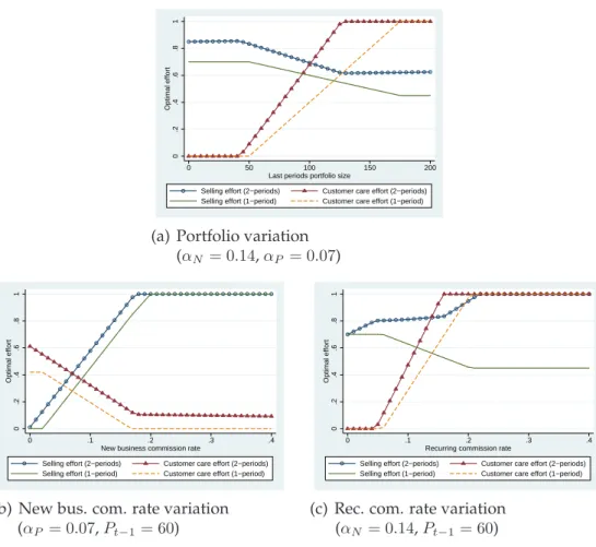
In other words, the result of Theorem 2.4 indicates that in the 2-period case, an increase of the new business commission rate has a positive effect on the sales effort and a negative effect on the customer care effort unless the recurring commission rate raises beyond a certain critical value. Be- yond this point, an increase in the new business commission rate leads to a decrease in the selling effort, resulting in the opposite effect to that presumably desired. Instead, the effort spent on customer care increases.
Even ifαP is still below the critical point, the higher the recurring commis- sion rate, the smaller the marginal effect of an increase in the new business commission rate. This result is in line with general intuition, as the agent
probably feels less willing to spend additional effort on selling if the re- curring commission rate is comparably high (and thus, the financial loss of not retaining a customer is quite severe).
2.2.2 Predictions from Simulated Data
As already pointed out above, it is impossible to calculate closed-form so- lutions for the marginal effect of the recurring commission rate or the last year’s portfolio on the optimal effort choice of the agent. I will now, there- fore, discuss the effects of changes inαP andPt−1, respectively, using sim- ulated data. It should be noted that the discussion of the 2-period results based on the simulated data is not meant to be a rigorous proof regarding the properties of the solution given in Theorem 2.3. Due to the depen- dency between the optimal effort and the chosen parametrization, some scenarios (e.g., that the root of the first derivative of the agent’s problem with respect to etN or etP does not mark a maximum but a minimum) are not discussed here. Instead, I will focus on those settings that resemble a ”real-life” scenario, disregarding some theoretical artifacts that may oc- cur. In Figure 2.2, we see the results of the numerical calculations, i.e., the formulas derived above were used to calculate the optimal selling and customer care effort under different scenarios. In order to calculate these values, I make some assumptions regarding the input-parameters. The choice was based on considerations regarding an appropriate relative re- lation between the parameters, although the overall level is fairly arbitrary as one could easily scale all parameters up or down without changing the qualitative, relational shape of the curves. As I assume the effort to be between 0 and 1, I chose the set of parameters to be close to 1 in order to maintain a common effect-level. Furthermore, if possible, I also tried to lean on the data-set I will use in the next section. In particular, I chose τ = 0.1, κ = 1.1, δ = 0.5, cN = 2, cP = 1, s = 0.5, σ2P = 0.1, βN = 10and r = 0.1. Thus, I assume a churn rate of 10%, which the agent can reduce (assuming a customer care effort of 1) to 1% (i.e., 10%∗(1.1−1)) due to
0.2.4.6.81Optimal effort
0 50 100 150 200
Last periods portfolio size
Selling effort (2−periods) Customer care effort (2−periods) Selling effort (1−period) Customer care effort (1−period)
(a) Portfolio variation (αN = 0.14,αP = 0.07)
0.2.4.6.81Optimal effort
0 .1 .2 .3 .4
New business commission rate
Selling effort (2−periods) Customer care effort (2−periods) Selling effort (1−period) Customer care effort (1−period)
(b) New bus. com. rate variation (αP = 0.07,Pt−1= 60)
0.2.4.6.81Optimal effort
0 .1 .2 .3 .4
Recurring commission rate
Selling effort (2−periods) Customer care effort (2−periods) Selling effort (1−period) Customer care effort (1−period)
(c) Rec. com. rate variation (αN = 0.14,Pt−1= 60)
Figure 2.2: Results from simulated data with βN = 10, τ = 0.1, δ = 0.5, s = 0.5,κ= 1.1,cN = 2,cP = 1,σP2 = 0.1,r= 0.1
the choice of κ = 1.1. I assume that the agent values the expected return of the next period with one-half. The cost associated with exerting effort on selling is assumed to be twice as large as the customer care effort (e.g., due to required customer visits prior to the signing of a contract and ad- ministrative one-off costs). The cost substitution factor is set to 0.5which is roughly one-third of the maximal, full-substitution value of√
2. I base this on the assumption that agents are not always in an ”either/or” situa- tion regarding how they spend their time but rather have some flexibility in their daily schedule. The uncertainty regarding the portfolio develop- ment is set to 10% of the portfolio managed. As unexpected changes in the portfolio development are rare and small, this value seems reasonable.
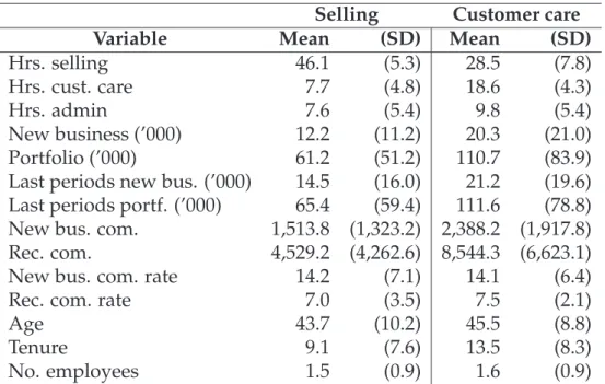
As the variance of the new business production error term is not required for the calculations, I omit it here. Regarding the scaling factor of the new business production βN, I try to be close to the data-set I will use in the next section. As we can see in Table 2.3, the average new business produc- tion is around EUR 14,000 and the average portfolio size is EUR 75,000. To keep a similar ratio in the simulated data, I set βN = 10in all cases and Pt−1 = 60in those cases where we analyze the commission rate variations (see Figures 2.2(b) and 2.2(c)). Also the choice ofαN andαP draws on the field data. In Figure 2.2(a), I set the commission rates to14%and7%for the new business and the recurring commission rate, respectively. In Figures 2.2(b) and 2.2(c), the same values are used for the non-variable commis- sion rate (i.e.,αP = 0.07in 2.2(b) andαN = 0.14in 2.2(c)).
As the optimal effort levels given in Theorem 2.2 and 2.3 are not restricted to values between 0 and 1, I set negative values to zero and values above one to 1. I will now show that this method (in most cases) leads to the unique maximum within the interval. As we will need the first order con- ditions of the agent’s problem that were already implicitly used for the proofs of Theorem 2.2 and 2.3, I will now explicitly state them here. The first order conditions for the 1-period case are
etN =αNβN −setP
cN (2.7)
etP =αPτ Pt−1−setN
cP (2.8)
and for the 2-period case
etN =B1etP +βN(αN +αPB2)
cN −βN2Kα2P (2.9)
etP =B1eN +τ Pt−1(αP +αPB2)
cP −τ2Pt−12 KαP2 (2.10) withB1 =βNα2Pτ Pt−1K−sandB2 = (1−κτc)(δ+αPPt−1K)
NcP−s2 .
With these preliminaries at hand, I summarize in Table 2.2.2 the rules on how to project the different possible effort levels into the interval of al-
etN
<0 ∈[0,1] > 0
<0 etN =etP = 0 (2.10) withetN = 0 ≈etN = 0, etP = 1 etP ∈[0,1] (2.9) withetP = 0 Theorem 2.3 (2.9) withetP = 1
>0 ≈etN = 1, etP = 0 (2.10) withetN = 1 etN =etP = 1 Table 2.1: Decision rules how to project the calculated optimal effort into the interval of [0,1] for the 2-period case
lowed values. Although I am interested mainly in the ”inner solutions” of the agent’s problem, i.e., where Theorem 2.3 applies, I will briefly discuss why the projection rules as described in Table 2.2.2 lead to the optimal ef- fort allocation within the given interval. Due to the inverted U-shape with respect to etN oretP of the agent’s problem, it is clear that if the vertex of the parable lies outside of [0,1], the maximum within this interval is at- tained at the boundaries, i.e., at 0 for negative optimal effort values and at 1 for positive optimal effort values. By setting the effort to values other than the calculated optimum, the equilibrium effort as given in Theorem 2.3 is no longer attained. Instead, if only one of the two effort values is set to its boundary value, we can use equation (2.9) or (2.10), respectively, to calculate the corresponding optimal effort. If both calculated optimal efforts are above (below) the upper (lower) boundary, setting one of them to one (zero) increases (decreases) the corresponding other effort level (as for most parameter constellations, B1 < 0and the denominators are pos- itive, there is a negative relation betweenetN andetP as one would expect due to the cost substitution between the two tasks. Therefore, decreasing (increasing) one of the efforts increases (decreases) the other one. Only in those cases where one value is above the upper and the other is below the lower boundary, might there be two ”second best” optima, depending on which of the two values is set to the boundary first (as the decrease (increase) of one effort could theoretically lead to the other value being pushed above (below) the boundary). As these nonetheless lie close to- gether due to the continuous nature of the equations, this does not change the qualitative direction of the results. The same argument applies to the 1-period case.