Workload modeling for parallel computers

(1)

Workload Modeling for Parallel Computers

Baiyi Song

Robotic Research Institute Section Information Technology

The University of Dortmund

A thesis submitted for the degree of Doktor-Ingenieur

(2)

(3)

Acknowledgements

I want to thank all those who made this work possible by their supports.

In particular, I want to express my appreciation to my doctorial advisor, Prof. Dr.-Ing. Uwe Schwiegelshohn, for the source of instructive guidance and supports over the past years.

I am grateful to all people at Robotic Research Institute at the University of Dortmund for the excellent working atmosphere. Especially, I would also like to thank Dr.-Ing. Ramin Yahyapour, whose efforts and expertise help me to finish my study. I would like to express my gratitude to Dipl.-Inform.

Carsten Ernemann, who give me many helpful suggestions and supports.

I would also like to thank the Graduate School of Production Engineering and Logistics at the University of Dortmund, which provides me not only the financial supports but also the broad contacts with other departments.

I would like to thank many of my chinese friends with them I had a pleasure time in Dortmund.

At last, I would like to thank my parents, my wife and my son, who always encourage me with their love, belief and patience.

(4)

(5)

Abstract

The availability of good workload models is essential for the design and analysis of parallel computer systems. A workload model can be applied directly in an experimental or simulation environment to verify new scheduling policies or strategies. Moreover, it can be used for extrapolating and predicting future workload conditions. In this work, we focus on the workload modeling for parallel computers. To this end, we start with an examination of the overall features of the available workloads. Here, we find a strong sequential dependency in the submission series of computational jobs. Next, a new approach using Markov chains is proposed that is capable of describ- ing the temporal dependency. Second, we analyze the missing attributes in some workloads. Our results show that the missing information can be still recovered when the relevant model is trained from other complete data set. Based on the results of overall workload analysis, we begin to inspect the workload characteristics based on particular user-level features. That is, we analyze in detail how the individual users use parallel computers.

In particular, we cluster the users into several manageable groups, while each of these groups has distinct features. These different groups provide a clear explanation for the global characteristics of workloads. Afterwards, we examine the user feedbacks and present a novel method to identify them.

These evidences indicate that some users have an adaptive tendency and a complete workload model should not ignore the users’ feedbacks. The work ends with a brief conclusion on the discussed modeling aspects and gives an outlook on future work.

(6)

(7)

List of Figures

2.1 A job is represented by a rectangle in our study. . . 8

2.2 A job is scheduled by a scheduling system. . . 9

2.3 A medium number of users submit jobs to a parallel system. . . 9

2.4 The global workload modeling structure . . . 12

2.5 Histogram of job runtime . . . 14

2.6 Histogram of job parallelism in the KTH workload . . . 15

2.7 A novel workload model structure . . . 16

3.1 Continuous job submissions . . . 23

3.2 Temporal relation in the sequence of the parallelism . . . 25

3.3 Temporal relation in the sequence of the runtime . . . 26

3.4 Process of correlated Markov chains model . . . 27

3.5 Comparison of modeled and original distributions of runtime and parallelism . . . 33

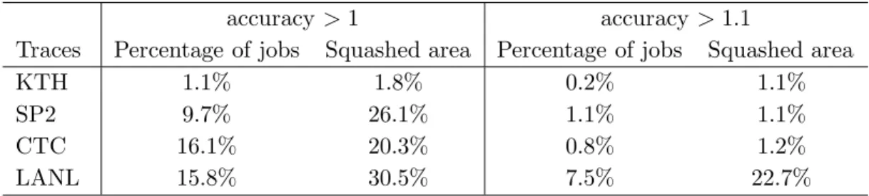
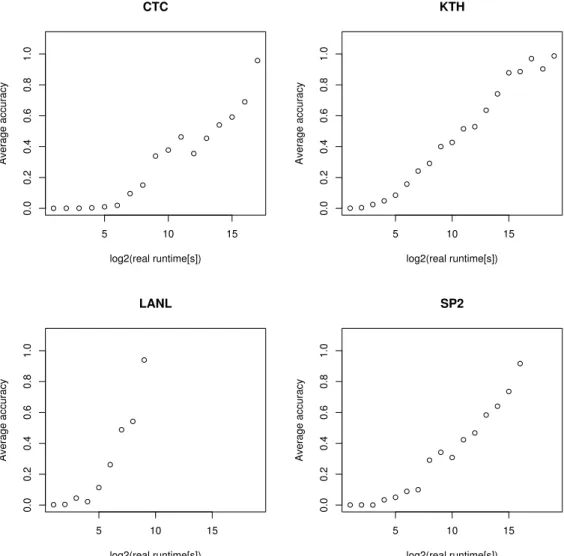
4.1 The relations of the accuracy to the real runtime. Here, only the jobs whose accuracies smaller than 1.1 are considered. . . 40

4.2 Comparison of modeled (SIM) and original (REAL) accuracies . . . 44

4.3 Comparison of modeled (SIM) and original (REAL) estimated runtime . 44 4.4 The relations between the real runtime and the parameters of the Beta distributions for KTH. The relations similar for the traces of SDSC SP2 and CTC . . . 45

4.5 Comparison of the synthetic (SIM) real estimated runtimes (REAL) . . 47

4.6 Comparison of the synthetic (SIM) and real estimated runtimes (REAL) 47 5.1 Comparison of the average job parallelism for individual users . . . 52

5.2 Process of the MUGM model . . . 53

5.3 Algorithm for the P AM Clustering . . . 56

5.4 2 user groups are clustered in KTH with the MUGM model. . . 59

iii

(10)

5.7 4 user groups are clustered in LANL with the MUGM model. . . 63

6.1 Histogram of the number of waiting jobs in KTH . . . 71

6.2 Feedback discoveries in KTH . . . 74

6.3 Feedback discoveries in CTC . . . 75

6.4 Feedback discoveries in the time frame from 1pm to 4pm in KTH . . . . 76

7.1 Daily cycle in KTH. Left: the number of jobs in the different hours of day. Right: the average runtime in the different hours of day . . . 80

7.2 Weekday effect in KTH. Left: the number of jobs in the different days of week. Right: average runtime in the different days of week . . . 80

7.3 Combination of correlated Markov chain and the user group model . . 81

7.4 Application of Neural network for workload modeling . . . 82

(11)

List of Tables

2.1 Used workloads from the SWF Archive . . . 18

3.1 Percentage of neighboring jobs with the same parallelism values . . . 22

3.2 Example for deriving the states of the Markov chain for the parallelism 28 3.3 Dimensions of the Markov chains for the parallelism and the runtime . . 29

3.4 Correlationcor₀ andcor₁ in examined workloads . . . 31

3.5 Static Comparison of the modeled and the original workloads . . . 33

3.6 Comparison of the correlation of the parallelism and the runtime from the Markov chain model and the Lublin/Feitelson model . . . 34

3.7 Comparison of the autocorrelationρ1 of the parallelism and the runtime sequences from MCM, PDM, and the original workloads . . . 34

4.1 Summary of missing estimated runtime for the examined workloads . . . 38

4.2 Analysis of the jobs exceeding their real runtimes . . . 39

4.3 Summarized alignment of the estimated runtimes within the KTH, SDSC SP2, CTC workloads, total alignment: 82.7% . . . 41

4.4 Alignment of the estimated runtimes within the LANL and KTH workloads 42 4.5 Alignment of the estimated runtimes within the CTC and SDSC SP2 workloads . . . 43

4.6 Alignment of the modeled estimated runtime . . . 46

4.7 Maximum estimated runtime (hours) of the different traces . . . 46

4.8 Comparison of KS test results and difference of SA . . . 47

4.9 Comparison of synthetic estimated runtime and real estimated runtime . 48 5.1 Comparison of the numbers of users’ submissions . . . 52

5.2 The Details of user groups (SA%, # of Jobs%, # of Users%) identified by the MUGM model . . . 64

5.3 KS test results (D_n) of the modeled and the original workloads . . . 65

v

(12)

5.4 Comparison of the correlations between the modeled and the original workloads . . . 65 6.1 Considered variables for feedback analysis . . . 69 6.2 Discretization Results with 5 levels for # of waiting jobs in KTH . . . 71 6.3 Summary of discovered feedbacks in the examined workloads . . . 77

(13)

Nomenclature

Acronyms

AIC Akaike’s Information Criteria

ARIMA Auto-Regressive Integrated Moving Average CLARA Clustering Large Applications

FCFS First Come First Service

HMM Hidden Markov Model

KS Kolmogorov-Smirnov

MCM Markov Chain Model

MPI Message Passing Interface MPPs Massively Parallel Processors MUGM Mixed User Group Model PAM Partition Around Medoids PDM Probabilistic Distribution Model PVM Parallel Virtual Machine

SA Squashed Area

SIQR Semi-Inter Quartile Range SVM Support Vector Machine VLMC Variable Length Markov Chain

vii

(14)

Symbols

γ,β The parameters of Gamma distribution

a The dimension of Markov chain for parallelism b The dimension of Markov chain for runtime cor Pearson’s correlation coefficient

D The set of jobs

di The parameter set for jobi d^p_i The parallelism of job i d^r_i The runtime of job i d^u_i The ownership of the job i

J The number of users in the system K Users are clustered into K groups p, q The parameters of Beta distribution

(15)

Chapter 1

Introduction

1.1 Motivation

Many traditional science disciplines as well as recent multimedia applications are in- creasingly dependent upon powerful high-performance systems for the execution of both computationally intensive and data intensive simulations of mathematical models and their visualizations. Parallel computing in particular has emerged as an indispens- able tool for problem solving in many scientific domains during the course of the past fifteen years, e.g., weather forecasting, climate research, molecular modeling, physics simulations.

A parallel computer is a high-end machine designed to support the execution of parallel computational jobs. It can be composed of hundreds of high-speed processors, often called nodes. The processors are interconnected by a very fast network. A variety of parallel computers have been developed and are available to the user community.

This variety ranges from the traditional Massively Parallel Processors (MPPs), to distributed shared memory systems, to clusters or networks of stand-alone workstations or PCs, to even geographically dispersed meta-systems or Grids connected by high-speed Internet connections. Research and development efforts focus on building faster processors, more powerful memories at all hierarchy levels, and on building fast networks with higher bandwidth and lower latencies. All these efforts contributed to the broad deployment of high-performance parallel systems.

Complementary to the hardware advance is the availability of transparent, highly portable, and robust software environments like Message Passing Interface (MPI) and Parallel Virtual Machine (PVM). Such environments hide the architecture details from the end-users and contribute to the portability and robustness of parallel jobs across a variety of hardware substrates. The availability of such environments transforms

1

(16)

every intranet into a high performance system, thus increasing the user access to parallel systems. Recently, the concept of Grid computing has been promoted [25, 26].

Grid computing provides shared access to a potentially large number of geographically distributed heterogeneous computational resources which are made available by independent providers. Such Grids are used to solve large scale problems, which are otherwise intractable due to their diverse requirements in terms of computing power, memory and storage.

The availability of different parallel systems as well as the diversity of available hardware and software make the arbitration and management of resources among the user community a non-trivial problem. For example, a number of users typically attempt to use the system simultaneously; the requests of resources are variable in the parallelism of the applications and their respective computational and storage needs;

sometimes execution deadlines must be met. Therefore, efficient scheduling systems are required to manage parallel computer resources. It is the task of the scheduling system to resolve the resource conflicts between the different jobs that are submitted to the system. It has to meet users’ specifications and fulfill owners’ requirements. A typical task of a scheduling system is , e.g., allocating resources according to the user’s requirements (i.e., cater to the interests of a user) and maximize the system through- out (i.e., maximize system utilization, which is particularly important to amortize the cost of parallel computers). To this end, the scheduling system has to decide when to allocate resources for a particular job and when to delay a job in favor of executing others.

Here, workload modeling plays a vital role in designing scheduling systems. Since most parallel computers are very expensive machines, conducting extensive experiments on an actual installation to select suitable algorithms or testify new scheduling strategies is rarely an option. Instead, simulations are often executed to analyze new strategies. Therefore, a suitable realistic workload model is required that can be used for the simulation. It helps to compare different scheduling algorithms and explore the performance of the system in a multitude of scenarios. Because the performance of a system can only be interpreted and compared correctly with respect to the processed load, workload modeling, i.e. selecting and characterizing the load, is a central issue in performance evaluation.

Open Problems in Workload Modeling

The research presented in this work has been focused on workload modeling for parallel computers. Workload modeling has been subject to research for a long time, not only

(17)

1.1. MOTIVATION 3

in the field of parallel computers but also in many other applications, e.g., web server characterization, network traffic description. Reviewing the available literature about workload modeling, we found that the workload models can be generally classified into three classes according to the number of users in the applications:

(a) A large number of independent users (say, thousands of individuals, or even more) contribute to a workload, e.g., in the field of telecommunication, a probabilistic distribution model [28, 41, 43, 55] normally works because the workloads from many independent users usually can be regarded as samples from a certain classical distribution, like Gaussian or Poisson.

(b) Only a few users (say, less than 10 users) are the contributors of a workload, like peer to peer Computing and special chip design [6, 10], specific models are required to describe each individual user or workload. That is, every user is represented using either a different model or a different parameter setting.

(c) A medium number of users (say, hundreds of users) generate a workload. Cur- rently, the methods from class (a) and (b) are used, i.e., a general statistical model and a set of user-specific models [30, 35].

Since the user community of a parallel computer is medium, i.e. hundreds of users [23, 48, 49, 50], workload modeling for parallel computer belongs to the class (c). However, neither a general distribution model from class (a) nor a set of user- specific models from class (b) can work in this case. It is mainly because:

- A probabilistic distribution model is based on the assumption of independent sampling. However, when the size of user community is medium (hundreds of users), some users’ patterns may still be observed in the final mixed workload.

Therefore, the assumption of independent sampling may not hold any more and the retained patterns tend to be ignored by a distribution model.

- A general model describes the global characteristics of a workload. However, it does not consider individual user behaviors. Therefore, it can not provide a clear explanation to many phenomena in overall workloads from a user point of view.

- Due to the medium size of the user community, it is infeasible to apply a specific model for each individual user. Otherwise, the number of parameters will be too large and the scalability of the model will be lost.

(18)

Therefore, a more suitable model is required to analyze and characterize the workload of parallel computers. This is the focus of our work. We will propose a new model to address the complex behavior of users, to generalize similar submission behaviors and to consider the users’ feedback behaviors. More details will be given in the next section.

Contribution of the Work

The objectives of our new workload model are to provide an adequate representation of the workload and meanwhile to characterize the way that users interact with parallel computers. The presented work serves on the one hand as a basis for deriving new workload models, and on the other hand as a beneficial supplement to existing approaches as new scheduling systems for parallel computers may include such models to predict the future workload situation. Several important aspects are considered in our new workload model:

- We inspect the temporal relations between jobs. A new approach is proposed to address the temporal relation in job series of workloads.

- Some attributes in the available workloads are missing due to the different resource configurations. Here, we propose a parameterized distribution model to describe the relation between missing and existing attributes.

- We put forward to a novel method to cluster heterogenous users into groups, while each of these groups has distinct features. Thus, more complicated scenarios can be simulated for evaluations by adjusting the parameters of user groups.

- We introduce implicit influential factors as representatives to examine the users’

feedback behaviors. A linear model is used to model the feedbacks. With the model, the feedbacks can be identified and represented by a few parameters.

1.2 Organization of the Thesis

This thesis is organized as follows. Following this introduction, we discuss in Chapter 2 the details of workload modeling for parallel computers. Some essentials about performance evaluation using workload models are introduced and the traditional methods are presented. Based on the comparison of the existing approaches, a novel model structure is proposed.

(19)

1.2. ORGANIZATION OF THE THESIS 5

Chapter 3 is devoted to modeling temporal relations in overall workloads. We will describe the details of our new method. That is, two correlated Markov chains are proposed to depict the temporal relations and the parameter correlations. Before turning to the next chapter, the comparisons of static and dynamic characteristics are made to verify our correlated Markov chains method.

Chapter 4 deals with missing information in the existing workloads. Not all available workloads provide the same set of information needed for some scheduling systems.

Here, we take estimated runtime as an example to explain how the missing information is analyzed and modeled. The difference between estimated and real runtime is ex- plained and then a parameterized distribution is given to model the estimated runtime, which is missing in some workloads.

In Chapter 5, the method to characterize individual users is given. The challenges to model the individual submission behaviors are discussed. Next, a user-group based workload model is given and the detailed steps to construct the model are introduced and corresponding results are presented.

Chapter 6 discusses the users’ feedback behaviors. First of all, several implicit influential factors are introduced and then a descriptive model based on linear regression is proposed. Afterwards, the details of feedbacks identifications are given. The potential reason and implication of the feedbacks are discussed as well.

In Chapter 7, we demonstrate how these different modeling aspects can be combined and give the future direction about our research work. Several optional methodologies and models are discussed. To take an example, we explain how a new model is constructed by the combination of temporal relations and user groups. Finally, the dissertation ends with a brief conclusion.

(20)

(21)

Chapter 2

Workload Modeling for Parallel Computers

Modeling, i.e. analyzing and characterizing workloads, is an important task in designing scheduling systems for parallel computers, as the estimated or observed performance results depend on the characteristics of workloads. In this chapter, we will give a detailed description of the workload modeling problem in the field of parallel computers.

Based on a broad overview of relevant work, a new structure is proposed. It is a collection of several fundamental components to address different aspects of workloads.

Our new model can be adapted to meet particular situations given by the goals of specific evaluation study.

First of all, we shall give an explanation of a parallel environment which is considered in our work.

2.1 Parallel Computing Environment

Parallel Architecture

As we have mentioned, a parallel computer is a high-end machine, which is used to support the execution of parallel computational tasks. It is usually composed of hundreds of high-speed processors or nodes, which are interconnected by a very fast network.

There are many different kinds of parallel computers (or ”parallel processors”). They are distinguished by the kind of interconnection between processors (known as ”processing elements” or PEs) and between memories. In our work, we assume that a parallel system is composed of identical processors or nodes. This coheres with the observation that many large scale systems for computational purposes consist of predominantly homogeneous partitions [19].

7

(22)

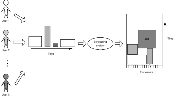
Job Description

A parallel computer is used for running computational tasks. Typically, these tasks use a certain amount of processors for a period of time. In our work, such a task is referred to as a job. A rectangle can be used to represent a job, with its width for parallelism and its length for the runtime as shown in Figure 2.1. Here, we use parallelism to refer to the number of processors or nodes used by a job (as shorthand for ”number of nodes”, or ”degree of parallelism”) and runtime for the span of time starting when a job commences execution and ending when it terminates (otherwise known as ”duration” or ”lifetime”). The product of runtime and parallelism of a job, which represents the total resource consumption (in CPU-seconds) used by the job, is called its squashed area. The term workload is referred to the data set recording historical job submissions. The termworkload model is referred to the statistical model to describe the real workloads.

Job

Parallelism Runtime

Figure 2.1: A job is represented by a rectangle in our study.

Scheduling Perspective

The scheduling problem of parallel computers is the composite problem of deciding where and when a job should execute. As we show in Figure 2.2, a scheduling system has to decide on which nodes (also indicated as the processor allocation or job scheduling problem) and in what order (also indicated as the process dispatching problem) the job will run. In our work, we consider space-sharing instead of time-sharing scheduling strategy, which is widely adopted by many parallel systems. Space-sharing scheduling restricts that two jobs executing concurrently must be disjoint. When a job is started on a machine, it runs to its end or is terminated. In our study, we specify that a job can not be stopped or interrupted unless it is finished, since many scheduling systems also follow this rule.

(23)

2.1. PARALLEL COMPUTING ENVIRONMENT 9

Time

Processors

Job

Start time

Allocated resources

Job

Figure 2.2: A job is scheduled by a scheduling system.

User Perspective

A medium number of users attempt to use parallel machine simultaneously, as it is shown in Figure 2.3. They submit jobs to the scheduling system and specify the details of resource requirements, including the number of processors, runtime, as well as some specific requirements. Usually, users make submissions from time to time. The scheduling system has no direct knowledge about the users’ next submissions. This is the typical online scenario. Users have their own object functions and their future submissions may be affected by their satisfaction with the parallel system.

...

User 1

User 2

User k

Scheduling system

Time

Processors Job

Time

Figure 2.3: A medium number of users submit jobs to a parallel system.

(24)

2.2 Performance Evaluation a Using Workload Model

As we have pointed out, workload features need to be taken into consideration when designing a scheduling strategy. Although the scheduling problem is conceptually the same across different systems and parallel workloads, the feasibility and performance of possible solutions are very sensitive to the workloads [21, 23, 46]. There is no scheduling algorithm that is suitable for all scenarios. In other words, scheduling must be done with caution because solutions need to be carefully tailored according to the workload characteristics. Therefore, the evaluation of scheduling algorithms under different workload situations is an important step in designing a suitable scheduling system and setting appropriate parameters. Basically, there are several methods for performance evaluation of a scheduling system:

Theoretical Analysis

The theoretical analysis is usually a worst-case study. It tries to provide a theoretical bound for certain performance criteria. The worst-case study is only of limited help as typical workloads on production machines normally do not exhibit the specific structure that will really cause a bad case. In addition, the theoretical analysis is often very difficult to apply to many scheduling strategies due to its complexity. Therefore, it is seldom adopted in evaluating scheduling systems for real cases.

Simulation-based Analysis

In practice, simulation-based performance evaluation is often carried out. It simulates the working procedure of scheduling systems with software tools and then the performance can be obtained from the simulation results. Several simulation tools have been developed, for example, SimGrid [33].

One of the most important considerations about simulation is its input. This is, which kind of workloads should be used as an input for a simulator in order to simulate the performance under a real environment? Researchers have at their disposal two valid methods for conducting simulation: it (1) uses real workload traces gathered from real machines and carefully reconstruct for use in simulation testing, or (2) creates a model from real workload traces and use the model either for analysis or for simulation. Next, we will explain both of them in detail.

(25)

2.2. PERFORMANCE EVALUATION A USING WORKLOAD MODEL 11

(1) Workload Traces for Simulations

A workload reflects areal test of a system: it records the job submissions precisely, with all their complexities even if they are unknown to the person performing the simulation.

The drawback is that a trace only reflects a specific usage of the machines: there are always doubts whether the results from a certain trace can be generalized to other situations. Moreover, the simulation of a scheduling system under different traces can be problematic. One reason is that if there are no enough jobs in a workload, the according simulation will not reflect the realistic performance of a scheduling system under heavy load. Since the traces were usually obtained from different resource configuration: it will be meaningless to conduct a simulation for a machine with 200 nodes using a trace obtained from a 100-node machine. It is because the trace will not contain the jobs whose nodes requirements are more than 100, which is obviously not true for the 200-node machine in practice. Another disadvantage is it is hard to change the characteristics of certain workload attribute(s), and even when it is applicable, it may be problematic. For example, it is difficult to increase the average runtime by adjusting the workload traces themselves. Increasing arriving rate by reducing the average inter- arrival time can be a problem, since the daily load cycle shrinks as well. If a model decomposes arriving rate and daily cycle, it will be feasible to adjust arriving rate as expected while keeping daily cycle unchanged.

(2) Workload Model for Simulations

In comparison with using traces, simulation using workload model has a number of advantages [17]:

- Model parameters can be adjusted stepwise, so that the investigation of individual settings can be performed while keeping other parameters constant. The stepwise parameter setting even allows the system designer to test how a system is sensitive to different parameters. It is also possible to select model parameters that are expected to match the specific workload at a given site.

- In many cases, only one experiment is not enough. Normally, more experiments are conducted in order to obtain certain confidential intervals. For example, a workload model can be applied several times with different seeds for random number generators.

- Finally, a workload model can lead to new designs of scheduling systems. A model is a generalization of a real workload and it is easy to know which parameters are correlated with each other because this information itself is part of the model.

(26)

With the deeper knowledge of workloads, the existing algorithms can be improved and even new methods can be derived. For instance, one can design a set of resource access policies that are parameterized by the settings of the workload model so that suitable resource policies are selected for different situations.

The key point of a workload model is its representativeness. That is, to which degree does the model represent the workload that the system will encounter? How are the crucial characteristics incorporated into the model? The answers depend not only on the methodology to build the model but also on the degree of details the model considers. In the next section, we will give a short overview on the existing methodologies for workload modeling in the domain of parallel computer.

2.3 Problems with Existing Approaches

Previous research focused on summarizing the overall features of the workload on a parallel computer [9, 36] as shown in Figure 2.4. Usually, the global characteristics of workload attributes are analyzed and certain methods are applied to summarize them.

Workload trace

Global Workload

model

Synthetic workload

Figure 2.4: The global workload modeling structure

The summaries are a collection of distributions for various workload attributes (e.g., runtime, parallelism, I/O, memory). By sampling from the corresponding distributions, a synthetic workload is generated. The construction of such a workload model is done by fitting the global workload attributes to theoretical distributions. Normally, it is done by comparing the histogram observed in the data to the expected frequencies of the theoretical distribution. The modeling methods usually fall into three families [29]:

Moment-based: The kth moment of a sequence x₁, x₂, . . . , xn of observations is defined by m_k = _n¹P

x^k_i. Important statistics derived from moments include:

(a) the mean, which represents the ”center of gravity” of a set of observations:

x = _n¹ P

xi; (b) the standard deviation, which gives an indication regarding the degree to which the observations are spread out around the mean: s =

(27)

2.3. PROBLEMS WITH EXISTING APPROACHES 13

q 1 n−1

P(xi−x)²; (c) the coefficient of variation, which is a normalized version of standard deviation: cv=s/x.

Percentile-based: Percentiles are the values that appear in certain positions in the sorted sequence of observations, where the position is specified as a percentage of total sequence. Important statistics derived from percentiles include:

(a) the median, which represents the center of the sequence: it is the 50th percentile, which means that half of the observations are smaller and half are larger;

(b)quartiles (the 25, 50, and 75 percentiles) and deciles (percentiles that are mul- tiples of 10). These give an indication of the shape of the distribution; (c) the Semi-InterQuartile Range (SIQR), which gives an indication of the spread around the median. It is defined as the average of distances from the median to the 25 percentile and to the 75 percentile.

Mode-based: The mode of a sequence of observations is the most common value observed. This statistic is obviously necessary when the values are not numerical, e.g., when they are user names. It is also useful for the distributions that have strong discrete components.

Here, we give several examples to explain how the classical methods are applied to model the workloads. Since the runtime and the parallelism of jobs are two of the most important attributes for many parallel systems [1,47,58], we focus on them in our study. The modeling of job arrival process is equally important and has been addressed by many papers, see [9,35] for more detailed information about the job arriving process modeling.

As mentioned earlier, the jobruntimeis the duration that a job occupies a processor set. The runtime histogram of KTH is shown in Figure2.5. It can be seen that runtime values usually spread from 1 to over 10⁵ seconds. Such a distribution characteristic is called heavy-tail and can be formally defined as follows: a random variable X is a heavy-tailed distribution if

P[X > x]∼cx^−α, as x→ ∞,0< α <2

wherec is a positive constant, and ∼means that the ratio of the two sides tends to 1 forx→ ∞. This distribution has infinite variance, and ifα≤1 it has an infinite mean.

To model the heavy-tail runtime, Downey [15] proposed a multi-stage log-normal distribution. This method is based on the observation that the empirical distribution of runtime in log space was approximately linear. Jan et al. [30] proposed a more general model by using a Hyper-Erlang distribution for runtime. They used moment estimation

(28)

to model the distribution parameters. Feitelson [22] argued that a moment estimation may suffer from several problems, including incorrect representation of the shape of the distribution and high sensitivity to sparse high value samples. Instead, Lublin &

Feitelson [36] selected a Hyper-Gamma distribution. They calculated the parameters by Maximum Likelihood Estimation.

KTH

runtime[s]

Frequency 050010001500

1 10¹ 10² 10³ 10⁴ 10⁵

Figure 2.5: Histogram of job runtime

Another important aspect of workload modeling is the jobparallelism, that is, the number of nodes or processors a job needs for execution. It has been found that the job parallelism in many available workloads displays two significant characteristics [15,21]:

(1) the power of 2 effect, as jobs tend to require power of 2 processor sets; (2) a high number of sequential jobs that require only one processor. These two features can be seen in Figure 2.6 clearly. It has been found empirically that these effects would significantly affect the evaluation of scheduling performance [35]. To describe these two features, a harmonic distribution is proposed in [21] which emphasize small parallelism and the other specific sizes like power of 2. Later, Lublin and Feitelson used job partitions to explicitly emphasize the power of 2 effects in the parallelism [36].

Besides the isolated modeling of each attribute, the correlations between different attributes were addressed as well. For instance, it has been found [30] that the runtime and the parallelism embody a certain positive correlation. That means the jobs with high parallelism tend to run longer than those with lower parallelism. Lo et al. [35]

demonstrated that the neglecting of correct correlation between job size and runtime yields misleading results. Thus, Jann et al. [30] divided the parallelism into subranges and then created a separate model of the runtime for each range. Furthermore, Lublin

(29)

2.3. PROBLEMS WITH EXISTING APPROACHES 15

KTH

parallelism Frequency 02000400060008000

1 2¹ 2² 2³ 2⁴ 2⁵ 2⁶ 2⁷

Figure 2.6: Histogram of job parallelism in the KTH workload

& Feitelson [36] considered the correlation according to a two-stage Hyper-Exponential distribution.

Although these models can provide the general description of a real workload, they have several serious drawbacks:

- Although static features can be characterized using probabilistic distributions, the temporal relation in job series is lost. A distribution model is based on the assumption of independent job submissions. As we mentioned earlier, due to the medium-sized user community, many user-level behaviors can still stay. Thus, such an assumption may not hold.

- The global level characterization does not provide an explicit explanation for user or user groups’ behaviors and thus could not help to relate the global workload metrics with user groups. For example, a Hyper-Exponential distribution is used to describe the heavy-tailed runtime in parallel machine, but it can not inter- pret how this tail is generated; the high fraction of serial jobs is addressed by a harmonic distribution but it fails to explain where these serial jobs come from.

- User feedback on the quantity of service or system state is ignored. To take a simple example, some users may continuously submit jobs only if their previous jobs are finished. As a result, the submission of users is dependent on the scheduling results - a static model obviously does not address this point.

Based on the investigation of the existing models, we propose a novel workload model in the next section.

(30)

2.4 Proposal of a New Workload Model

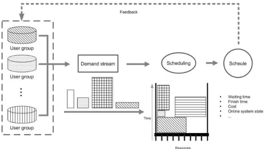
According to analysis of the drawbacks of the existing models, we put forward to a new model. The structure of our model is shown in Figure 2.7. Instead of a general

Figure 2.7: A novel workload model structure

description of workload, our model considers several user groups, where distinctive submission behaviors are represented. For example, some users always submit the jobs with longer runtime; others tend to submit jobs requiring only one node. Our new model addresses the feedback of users. That is, users have adaptive behaviors - both the submission and profile of a job may be affected by quality of service or system state.

In detail, the new model will be constructed according to the following steps:

Temporal Relations: First of all, we restrict ourselves on the global level of workload modeling. Previous models ignored the temporal relation. Hence it would be interesting to know whether there exist some temporal relation evidences. Here, several classical time series methods are considered, like ARIMA, Neural Network, Markov Chains.

Missing Information: Missing information is another problem to be dealt with when the global level modeling is considered. Due to different resource configurations and scheduling systems, certain attributes of the existing workloads are missing. Since there are not so many workloads available, we need to analyze

(31)

2.4. PROPOSAL OF A NEW WORKLOAD MODEL 17

these missing attributes and recover them so that the simulations based on different workloads can be performed. Here we consider the methods from classical statistics as options, e.g., analysis of variance, regressions.

User Groups: After analyzing the global workload features, we begin to the investigate user-level characteristics. Since the user community of parallel computers is medium-sized, it would be quite beneficial to associate the final workload with the user or user groups. With the user-level information it may be possible to explain those global features we have found and explore the effects of specific users on performance metrics. To identify user groups, the clustering methods from the data mining community can be applied, e.g., k-means, model-based clustering.

Additional Influencing Factors: Next, we investigate the possible factors that affect user submissions. Because of the lack of explicit influential factors, we need to derive certain implicit variables and try to identify feedback evidences. To this end, several techniques are tried to determine and measure the variable relations, like correlation and factor analysis.

Before we are turning to detailed explanation of our methods in the following chap- ters, we introduce the data set and software tools used in this work.

Workload Traces

The workload traces used in our work are from Standard Workload Archive [51]. They were collected from a variety of machines at several national labs and supercomputer sites in the United States and Europe. The type of workloads at these sites consisted of various scientific applications ranging from numerical aerodynamic simulations to elementary particle physics. Trace data were collected through a batch scheduling agent such as the Network Queuing System, LoadLeveler, PBS, or EASY [32]. Here, we briefly summarize the machine architecture, user environment, and scheduling policies of each workload:

KTH IBM SP-2: The Swedish Royal Institute of Technology IBM SP-2 machine with 100 nodes connected by a high performance switch. The trace came from June 1996 to May 1997 with scheduling managed by IBM’s LoadLeveler.

CTC IBM SP-2: The Cornell Theory Center IBM SP-2 machine. The trace came from September 1996 to August 1997 with scheduling managed by IBM’s LoadLeveler.

(32)

LANL CM-5 This log contains two years worth of accounting records produced by the DJM software running on the 1024-node CM-5 at Los Alamos National Lab (LANL). The trace came from periods: October 1994 to September 1996.

SDSC IBM SP-2: The San Diego Supercomputer Center houses a 128 node IBM SP-2 machine. This trace was taken from May 1998 to April 2000.

SDSC Intel Paragon 95: The San Diego Supercomputer Center houses a 416 node Paragon machine. The scheduling policies were implemented through the Network Queuing System (NQS). The trace was taken from December 1994 to December 1995.

SDSC Intel Paragon 96: The resource configuration was the same as for SDSC Intel Paragon 95. This trace was taken from from December 1995 to December 1996.

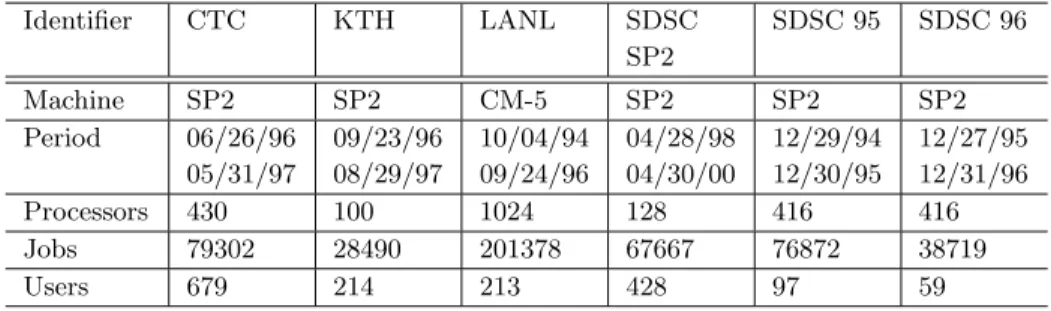
In Table 2.1these traces are summarized for later references.

Identifier CTC KTH LANL SDSC

SP2

SDSC 95 SDSC 96

Machine SP2 SP2 CM-5 SP2 SP2 SP2

Period 06/26/96 05/31/97

09/23/96 08/29/97

10/04/94 09/24/96

04/28/98 04/30/00

12/29/94 12/30/95

12/27/95 12/31/96

Processors 430 100 1024 128 416 416

Jobs 79302 28490 201378 67667 76872 38719

Users 679 214 213 428 97 59

Table 2.1: Used workloads from the SWF Archive

Software Tool

The tool used in our work is R [5], which is a language and environment for statistical computing and graphics. It is a GNU project which is similar to the S language and environment which was developed at Bell Laboratories (formerly AT&T, now Lucent Technologies) by John Chambers and colleagues. R can be considered as a different implementation of S. There are some important differences, but much code written for S runs unaltered under R.

We select R as our basic tool because R provides a wide variety of statistical (linear and nonlinear modeling, classical statistical tests, time-series analysis, classification, clustering, . . . ) techniques, and is highly extensible. It is especially useful for our task,

(33)

2.4. PROPOSAL OF A NEW WORKLOAD MODEL 19

which in many cases is a try-out task. With R we can directly try various methods for modeling task.

R is good at producing well-designed publication-quality plots, including mathematical symbols and formulae where needed. Therefore, we can visualize the job submissions and identify the important aspects of data.

In addition, R is available as Free Software under the terms of the Free Software Foundation’s GNU General Public License in source code form. We can obtain it freely from Internet, read and change the source code according to our needs.

(34)

(35)

Chapter 3

Investigation of Temporal Relations

As we have mentioned, workload modeling play a vital role in designing and developing the scheduling system for parallel computers. Therefore, we proposed a novel workload model in the last chapter. Our model consists of several fundamental components to address different aspects of the modeling problem. From this chapter on, we shall describe each component in detail.

In this chapter, we will focus on the temporal analysis of workloads. Many workload models use probabilistic distributions, which are based on the assumption of independent sampling. Therefore, we will verify whether such an assumption still holds or not in a parallel computer environment. Actually, our evidences show that there are strong temporal relations in job submission series. A straightforward methodology to model temporal relations is time series analysis, e.g., ARIMA. However, due to the relations between the job parameters, a direct application of the classical methodologies is infeasible. Hence, we propose a new approach not only to address the temporal relation but also to consider the parameter correlations. The experimental results will be discussed at the end of this chapter.

3.1 Observations on Temporal Relations

A temporal relation is an inter-propositional relation that communicates the ordering in time of events or states. Several temporal phenomena in job submission series have already been found. One of them is repeated submission [21], namely, users do not submit one job once but several similar jobs in a short time frame. Since there are only a medium number of users submitting jobs, such duplicated submissions can still

21

(36)

be distinguished in the overall job submissions. It can be seen from Table 3.1 that a large number of neighboring jobs share the same parallelism values. This continuous occurrence demonstrates that the assumption of independent sampling is not correct.

Percentage (%)

CTC 48.2

KTH 37.5

LANL 46.8

SP2 57.2

SDSC95 49.3

SDSC96 45.6

Table 3.1: Percentage of neighboring jobs with the same parallelism values

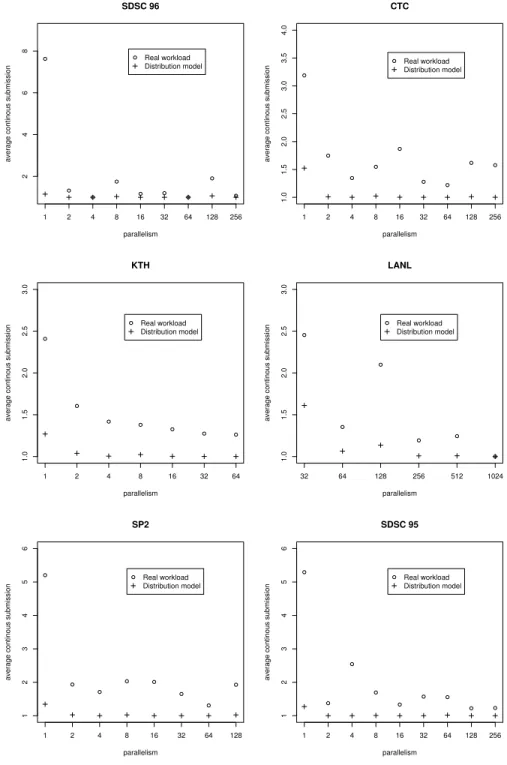
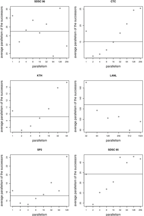
In addition, we find that not all jobs are submitted with the same continuity. For a job seriesJ in a workload, we extract the parallelismuj ∈U for each jobj. We examine the average continued occurrences of parallelism values in the sequence U. That is, the number of direct repetitions is considered for each parallelism value inU. Note that we consider all job submissions instead of the jobs submitted by the same users. As the existing workloads contain predominantly jobs with the power of 2 parallelism values, we restrict our examination on such jobs requiring 1 node, 2 nodes, 4 nodes, etc. In Figure 3.1 the average subsequent appearances of job parallelism in real workloads is shown. As a reference, the average number of occurrences is provided if a multinomial distribution model is used for modeling parallelism. The details of the application of multinomial distribution can be found in [14]. This strategy models each parameter independently according to the statistical occurrences in an original trace. It can be seen that the sequences of the same parallelism values occur significantly more often in a real workload than it would be in a distribution model. This indicates that a simple distribution model does not correctly represent such an effect. Furthermore, it can also be seen that the jobs with less parallelism have a lager average repeating than that of jobs requiring more nodes in the real traces. That is, the jobs with less parallelism have a higher probability to be repeatedly submitted.

Even if those continuous appearing elements inU are removed, sequential dependencies can still be found. To this end, only one element is kept for each sequence of the identical parallelism values. For example, an excerpt in a series of parallelism of 1, 1, 1, 2, 2, 5, 5, 5, 8, 16, 16, 16, 2, 2 is changed to 1, 2, 5, 8, 16, 2 after the removal of repeated items. Here, the jobs with parallelism values that are not the power of 2 are considered as well. Suppose the transformed parallelism sequence is U⁰. Next, we

(37)

3.1. OBSERVATIONS ON TEMPORAL RELATIONS 23

SDSC 96

parallelism

average continous submission

1 2 4 8 16 32 64 128 256

2468

Real workload Distribution model

CTC

parallelism

1 2 4 8 16 32 64 128 256

1.01.52.02.53.03.54.0

KTH

parallelism

1 2 4 8 16 32 64

1.01.52.02.53.0

LANL

parallelism

32 64 128 256 512 1024

1.01.52.02.53.0

SP2

parallelism

1 2 4 8 16 32 64 128

123456

SDSC 95

parallelism

1 2 4 8 16 32 64 128 256

123456

Figure 3.1: Continuous job submissions

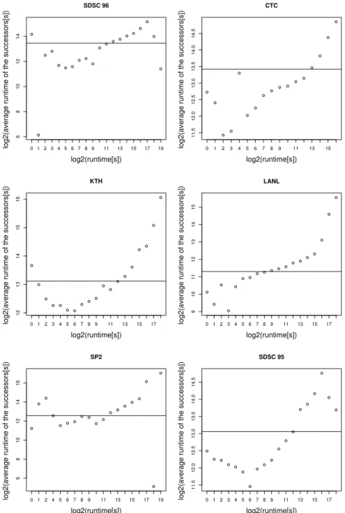
transform U⁰ to U⁰⁰ by U⁰⁰ = {2^blog²^(u⁰ⁱ^)c|u⁰_i ∈ U⁰}. That is, each parallelism value is rounded to the nearest lower power of 2. For each distinct parallelism value inU⁰⁰, we

(38)

calculate the average parallelism value requested by its successor inU⁰. The results are shown in Figure 3.2. The line in the figure is the overall average parallelism value as a reference. It can be seen that the successors of the jobs with a large node requirements also tend to request a large number of nodes for the most workloads. However, the behaviors for SDSC96 and SP2 are different from the others, the reason is not clear yet.

There is a temporal relation in the runtime series as well. To examine it, we group all the jobs by the integer part of the logarithm (based on 2) of their runtimes and for each group the average runtime of its successors has been calculated. The results are shown in Figure 3.3.

Such sequential dependencies may become very important for optimizing many scheduling algorithms, like e.g. Backfilling [24]. For instance, a scheduling algorithm can utilize probability information to predict future job arrivals. Such data can be included in heuristics about current job allocations. Therefore, a method to capture the sequential dependencies of workloads would be beneficial.

3.2 Modeling using Markov Chain Model

There are several classical methods to model a stochastic process. For example, Auto- Regressive Integrated Moving Average (ARIMA) time series models form a general class of linear models that are widely used in modeling and forecasting time series [7].

ARIMA has been successful applied in many applications where the continuous time systems are considered. However, since most parallelism values in the workloads are usually discrete, the ARIMA model is not suitable for our case. Another common approach is the use of Neural Networks to analyze and model sequential dependencies [11, 53]. But it is difficult to scale and extend such a model.

Therefore, a Markov chain model is chosen for modeling the described temporal patterns in Section 3.1. A Markov chain model has the important characteristic that the transition from one state to the next state depends on the previous state(s). To reduce the number of parameters in a model, we consider the application of first-order Markov chain. The first-order Markov chain can be described by a transition matrix.

The element (i, j) within the matrix describes the probability to move from state ito state j if the system is in statei.

In our workload model, we use two Markov chains to represent the parallelism and the runtime respectively. If these two Markov chains are independent, they can not express the correlation between the parallelism and the runtime. Thus, more structures are required to reflect the correlation.

(39)

3.2. MODELING USING MARKOV CHAIN MODEL 25

SDSC 96

parallelism

average parallelism of the successors

1 2 4 8 16 32 64 128 256

202224262830

CTC

parallelism

1 2 4 8 16 32 64 128 256

152025

KTH

parallelism

1 2 4 8 16 32 64

891011121314

LANL

parallelism

32 64 128 256 512 1024

80100120140160

SP2

parallelism

1 2 4 8 16 32 64 128

141618202224

SDSC 95

parallelism

1 2 4 8 16 32 64 128 256

2025303540

Figure 3.2: Temporal relation in the sequence of the parallelism

Similar requirements for correlating Markov chains also occur in other application areas [18, 39, 44]. For instance, advanced speech recognition systems use the so-called Hidden Markov Model (HMM) to represent not only phonemes, the smallest sound

(40)

SDSC 96

log2(runtime[s])

log2(average runtime of the successors[s]) 0 1 2 3 4 5 6 7 8 9 11 13 15 17 19

68101214

CTC

log2(runtime[s])

log2(average runtime of the successors[s]) 0 1 2 3 4 5 6 7 8 9 11 13 15

11.512.012.513.013.514.014.5

KTH

log2(runtime[s])

log2(average runtime of the successors[s]) 0 1 2 3 4 5 6 7 8 9 11 13 15 17

1213141516

LANL

log2(runtime[s])

9101112131415

SP2

log2(runtime[s])

6810121416

SDSC 95

log2(runtime[s])

11.512.012.513.013.514.014.5

Figure 3.3: Temporal relation in the sequence of the runtime

units of which words are composed, but also their combinations to words. The method to correlate different Markov models is called ”embedded” HMM, in which each state in the model (super states) can represent another Markov model (embedded states).

(41)

Data processing

Markov chain for parallelism constructing

Markov chain for runtime constructing

Markov chain correlating

Synthetic workload generation

Figure 3.4: Process of correlated Markov chains model

However, this method is not suitable to our problem, as it will dramatically increase the number of parameters. Consequently, the model becomes very hard to train. Hence, in the following we propose a new method to correlate two Markov chains without increasing the number of states.

Our model first builds two Markov chains independently, one for the parallelism and one for the runtime. Then the two chains are combined to address the correlation between parallelism and runtime. In Figure3.4the steps to build the correlated Markov chains model are shown.

3.2.1 Markov Chain Construction

Our method starts with constructing two independent Markov chains. Here, we explain how a Markov chain model for the parallelism is built, a similar method can be applied for the construction of the Markov chain for the runtime.

One of the key issues during the construction of a Markov chain is the identification of relevant states in the series. In our case, if all distinct values in the traces are specified as different states, the Markov chain would have a prohibitively high dimension transformation matrix. To this end, a small set of states are specified for the Markov chain for the parallelism.

Assume a sequence of n jobs where the series of the parallelism is described by the sequence T = {t₁, t₂,· · ·t_n}. Thus, the reduced sequence S = {s₁, s₂· · ·s_n} is constructed from T as follows:

si = 2^blog²^tⁱ^c, i∈[1, n] (3.1) Now, each distinct element in S can be considered as a separate state in the Markov

(42)

chain. The set of states Lof this Markov chain can be expressed as follows:

L={l₁, l₂,· · ·lq|q ≤n;∀i∈[1, q−1], j ∈[2, q], i < j: li< lj;∀c∈[1, q], lc∈S} (3.2) Using this transformation, the original sequence T is represented using S and L.

In order to consider the state changes in the original workload, we use U to denote the according transformation path of S. In fact, the sequence U is the corresponding indices of the elements inLcorresponding to the job sequence. In Table3.2an example is given to illustrate the process of reducing the distinct parallelism values.

Index 1 2 3 4

ti∈T 2 4 6 16

s_i ∈S 2 4 4 16

lj ∈L 2 4 16 -

ui ∈U 1 2 2 3

Table 3.2: Example for deriving the states of the Markov chain for the parallelism

WithU and L, the transition matrixE of the Markov chain for the parallelism can be calculated as: e_ij=p_ij/p_i, wheree_ij ande_i are

p_i = |{k|s_k =l_i, k= 1, . . . , n−1}| and (3.3) pij = |{k|s_k =li∧s_k+1=lj, k= 1, . . . , n−1}| . (3.4) The transformation fromT toS causes a loss of information about the precise parallelism, as they have been reduced to the power of 2 values. To record the information loss, aquality ratiocj is defined for each state in the Markov chain. This ratio indicates how often the real values in the original group are exactly equal to the representing value in this state of the chain. More precisely, the quality ratio is calculated by:

cj = |{i|ti =lj, i= 1, . . . , n}|

|{i|si =lj, i= 1, . . . , n}|. (3.5) The definition of the quality ratioscj,j∈[1, q] is used to generate the final synthet- ical parallelism of a job. If the system is in statej, the corresponding valuelj is used as the system output with the probability ofcj. With the probability of (1−cj) a uniform distribution between [lj, l_j+1] is used to create the final value for the parallelism.

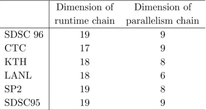
The same method can be applied to model the runtime. This yields a second Markov chain. As a short summary, the dimensions of the two matrices for the considered workloads are presented in Table 3.3.

(43)

Dimension of Dimension of runtime chain parallelism chain

SDSC 96 19 9

CTC 17 9

KTH 18 8

LANL 18 6

SP2 19 8

SDSC95 19 9

Table 3.3: Dimensions of the Markov chains for the parallelism and the runtime

3.2.2 Combination of Two Markov Chains

As we have mentioned, the runtime and the parallelism have a weak positive correlation in all examined workloads (except CTC), that is, the jobs requiring more nodes have longer runtimes on average [23]. Such a correlation has an impact on the performance of the scheduling algorithms as shown in [21]. Therefore, this correlation should be reflected in our model as a key feature.

To this end, these two independent Markov chains for the parallelism and the runtime need be combined to incorporate the correlation. A common approach would be the mergence of these two Markov chains into a single Markov chain. However, this would yield a very high dimension chain based on all combinations of the states in the two original chains. Such a Markov chain is very difficult to analyze and could not be scaled for incorporating additional job parameters.

In our approach, we combine these two chains by adjusting the state of transformation of one chain depending on the state transformation of the other chain. Here, we describe how the new state in the Markov chain for the parallelism is adjusted according to the latest transition in the chain for the runtime. Using the transformation of the runtime chain to affect the transition of the parallelism chain is similar.

The idea is that since the runtime and the parallelism are correlated, the transfor- mations of their corresponding Markov chains are related as well. For example, when the Markov chain for the runtime is in a state representing longer runtime, the state of the Markov chain for the parallelism would tend to move to a state requesting more nodes, when they are positive related, and vice versa. If the runtime changes dramatically in a chain, the parallelism would have a tendency to change correspondingly. As a result, the transformation of the states in the different Markov chains incorporates the correlation between their representing parameters.